A Novel Physics Informed Deep Learning Method for

Simulation-Based Modelling

Hasan Karali∗

Istanbul Technical University, Istanbul, 34469, Turkey

Mustafa Umut Demirezen†

ITU Aerospace Research Center, Istanbul, 34469, Turkey

M. Adil Yukselen‡

Istanbul Technical University, Istanbul, 34469, Turkey

Gokhan Inalhan §

Cranfield University, Bedford, MK43 0AL, United Kingdom

In this paper, we present a brief review of the state of the art physics informed deep learning

methodology and examine its applicability, limits, advantages, and disadvantages via several

applications. The main advantage of this method is that it can predict the solution of the

partial differential equations by using only boundary and initial conditions without the need

for any training data or pre-process phase. Using physics informed neural network algorithms,

it is possible to solve partial differential equations in many different problems encountered in

engineering studies with a low cost and time instead of traditional numerical methodologies.

A direct comparison between the initial results of the current model, analytical solutions, and

computational fluid dynamics methods shows very good agreement. The proposed methodology

provides a crucial basis for solution of more advance partial differential equation systems and

offers a new analysis and mathematical modelling tool for aerospace applications.

I. Introduction

Since the beginning of aviation, aerial vehicles have evolved to perform faster operations at higher altitudes. Especially

with advances in unmanned vehicle control systems, propulsion systems and material technologies, these vehicles

have become platforms that offer extensive application prospects combining excellent characteristics of high speed,

maneuverability and survivability. Nowadays supersonic transports, next-generation supersonic UAVs and hypersonic

atmospheric reentry vehicles are the most prominent research topics in the fields of both aeronautics and astronautics

(see Fig. 1). The design and optimization of these complex systems have top priority due to the potential capabilities that

they offer in both civilian and military settings. However, modelling of these vehicles from a dynamics and performance

sense can be extremely challenging given the complexity of aerodynamics. In that perspective, machine learning

and simulation based modelling and design provides an enabling approach. Specifically, the existing approaches to

determining aerodynamic characteristics of complex vehicles highly depend on high order numerical simulations in

other words computational fluid dynamics (CFD) methods. Considering the time steps and grids used for the stability of

the solution, the processing loads, especially at high speeds, require a huge amount of computing power and processing

time. As a solution to this problem, in this paper we suggest and evaluate a physics informed deep learning model that

use artificial intelligence (AI) algorithms. Thanks to these algorithms, it will be possible to solve partial differential

equations in many different problems encountered in engineering studies with a low cost and time instead of traditional

methodologies such as CFD. In the near future, we think that this methodology that currently developing can be a

powerful alternative to classical analysis tools in the aerospace applications. In this study, we made a brief review of the

method and examined its applicability, limits, advantages, and disadvantages via several applications.

∗Research Assistant, Department of Aeronautical Engineering, karalih@itu.edu.tr, AIAA Student Member†Affiliated Professor, ITU Aerospace Research Center, umut@demirezen.tech‡Professor, Department of Aeronautical Engineering, yukselen@itu.edu.tr§BAE Systems Chair, Professor of Autonomous Systems and Artificial Intelligence, inalhan@cranfield.ac.uk, AIAA Associate Fellow

1

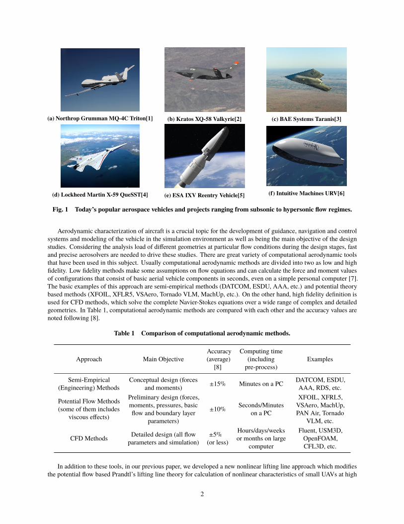
(a) Northrop Grumman MQ-4C Triton[1] (b) Kratos XQ-58 Valkyrie[2] (c) BAE Systems Taranis[3]

(d) Lockheed Martin X-59 QueSST[4] (e) ESA IXV Reentry Vehicle[5] (f) Intuitive Machines URV[6]

Fig. 1 Today’s popular aerospace vehicles and projects ranging from subsonic to hypersonic flow regimes.

Aerodynamic characterization of aircraft is a crucial topic for the development of guidance, navigation and control

systems and modeling of the vehicle in the simulation environment as well as being the main objective of the design

studies. Considering the analysis load of different geometries at particular flow conditions during the design stages, fast

and precise aerosolvers are needed to drive these studies. There are great variety of computational aerodynamic tools

that have been used in this subject. Usually computational aerodynamic methods are divided into two as low and high

fidelity. Low fidelity methods make some assumptions on flow equations and can calculate the force and moment values

of configurations that consist of basic aerial vehicle components in seconds, even on a simple personal computer [7].

The basic examples of this approach are semi-empirical methods (DATCOM, ESDU, AAA, etc.) and potential theory

based methods (XFOIL, XFLR5, VSAero, Tornado VLM, MachUp, etc.). On the other hand, high fidelity definition is

used for CFD methods, which solve the complete Navier-Stokes equations over a wide range of complex and detailed

geometries. In Table 1, computational aerodynamic methods are compared with each other and the accuracy values are

noted following [8].

Table 1 Comparison of computational aerodynamic methods.

Approach Main Objective

Accuracy

(average)

[8]

Computing time

(including

pre-process)

Examples

Semi-Empirical

(Engineering) Methods

Conceptual design (forces

and moments)±15% Minutes on a PC

DATCOM, ESDU,

AAA, RDS, etc.

Potential Flow Methods

(some of them includes

viscous effects)

Preliminary design (forces,

moments, pressures, basic

flow and boundary layer

parameters)

±10%Seconds/Minutes

on a PC

XFOIL, XFRL5,

VSAero, MachUp,

PAN Air, Tornado

VLM, etc.

CFD MethodsDetailed design (all flow

parameters and simulation)

±5%

(or less)

Hours/days/weeks

or months on large

computer

Fluent, USM3D,

OpenFOAM,

CFL3D, etc.

In addition to these tools, in our previous paper, we developed a new nonlinear lifting line approach which modifies

the potential flow based Prandtl’s lifting line theory for calculation of nonlinear characteristics of small UAVs at high

2

angles of attack [9]. It is a computationally efficient and high-precision nonlinear aerodynamic analysis method including

viscous effects towards both design optimization and mathematical modelling of small UAVs. This tool has been used

successfully in various applications as in the ARC UAV project. However, the method is valid for conventional aerial

vehicles operating in a subsonic, incompressible flow regimes that can be considered too narrow area for aerospace

applications. Detailed configurations including unconventional geometries can be solved most accurately in high Mach

and Reynolds number flight regimes with CFD methods which contain Navier-Stokes equations. As stated in Cummings

et al., a full aircraft solution easily consists of 10 million grid points that we try to calculate density, viscosity, pressure,

velocity (three components), temperature parameters for each time steps. Considering the coordinates of these points

and the number of operations to be repeated, it is imperative to use expensive high performance computing to track 100

million pieces of information. For instance, the flow simulation of a F-15 aircraft in the post-stall angle of attack during

spin takes thousands of hours of computer time, even on the CRAY XT3 supercomputer with over 4000 processors

[8]. As pointed in the NASA’s CFD Vision 2030 report, grand challenging problems are to drive the identification and

solution of the critical CFD barriers such as physics models of different flow regimes or high performance computing

limits may not be routinely achievable by 2030 [10]. Furthermore, Philippe Spalart of the Boeing Company estimates

that direct numerical simulation of full aircraft at flight Reynolds will not be available until 2080 with the current level

of technological development [11].

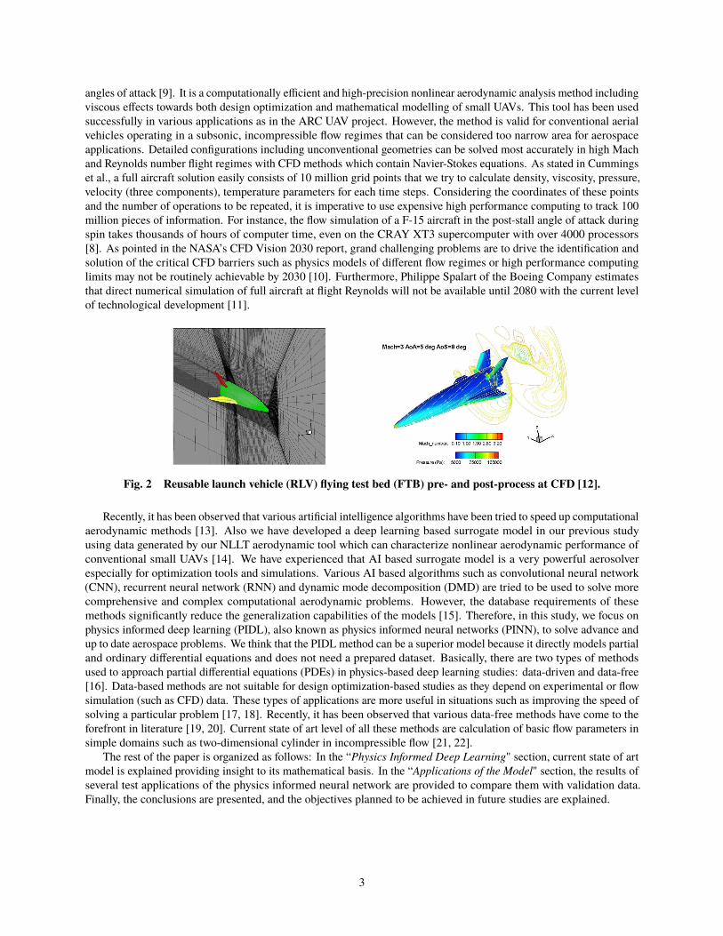
Fig. 2 Reusable launch vehicle (RLV) flying test bed (FTB) pre- and post-process at CFD [12].

Recently, it has been observed that various artificial intelligence algorithms have been tried to speed up computational

aerodynamic methods [13]. Also we have developed a deep learning based surrogate model in our previous study

using data generated by our NLLT aerodynamic tool which can characterize nonlinear aerodynamic performance of

conventional small UAVs [14]. We have experienced that AI based surrogate model is a very powerful aerosolver

especially for optimization tools and simulations. Various AI based algorithms such as convolutional neural network

(CNN), recurrent neural network (RNN) and dynamic mode decomposition (DMD) are tried to be used to solve more

comprehensive and complex computational aerodynamic problems. However, the database requirements of these

methods significantly reduce the generalization capabilities of the models [15]. Therefore, in this study, we focus on

physics informed deep learning (PIDL), also known as physics informed neural networks (PINN), to solve advance and

up to date aerospace problems. We think that the PIDL method can be a superior model because it directly models partial

and ordinary differential equations and does not need a prepared dataset. Basically, there are two types of methods

used to approach partial differential equations (PDEs) in physics-based deep learning studies: data-driven and data-free

[16]. Data-based methods are not suitable for design optimization-based studies as they depend on experimental or flow

simulation (such as CFD) data. These types of applications are more useful in situations such as improving the speed of

solving a particular problem [17, 18]. Recently, it has been observed that various data-free methods have come to the

forefront in literature [19, 20]. Current state of art level of all these methods are calculation of basic flow parameters in

simple domains such as two-dimensional cylinder in incompressible flow [21, 22].

The rest of the paper is organized as follows: In the “Physics Informed Deep Learning" section, current state of art

model is explained providing insight to its mathematical basis. In the “Applications of the Model" section, the results of

several test applications of the physics informed neural network are provided to compare them with validation data.

Finally, the conclusions are presented, and the objectives planned to be achieved in future studies are explained.

3

II. Physics Informed Deep LearningPhysics informed deep learning models can be defined as neural network algorithms that can combine data and

physics in the learning process by adding the residuals of a system of partial differential equations to the loss function

[23]. PIDL models consist of two basic algorithms: deep neural networks and automatic differentiation. A deep neural

network is formed by multiple layers between the input and output layers. In PIDL models, generally feed-forward neural

network (FNN) structure, which is simplest type of artificial neural network, is used. In this network the information

moves in only forward direction from the input nodes, through the hidden nodes and to the output nodes. If we update

the notation in our previous paper [14], the output of a layer can be formulated as follows:

I; = f(

, ;G; + 1;)

(1)

where f is the activation function, , ; is the weight matrix and 1; is the bias vector at the ;Cℎ layer. Activation

function decides which neurons will be activated, in other words what information would be passed to further layers. If

we extend this notation to include the entire algorithm [24], we obtain follows:

input layer: I0G = G ∈ R3in

hidden layers: I;G = f(

, ;I;−1G + 1;)

∈ R#; , for 1 ≤ ; ≤ ! − 1

output layer: I!G = ,!I!−1G + 1! ∈ R3out

where I! (x) : R3in → R3out be a ! -layer neural network, or a (! −1) -hidden layer neural network, with #; neurons

in the ; -th layer (#0 = 3in , #! = 3out ) .

Automatic differentiation is used to differentiate neural networks with respect to their input coordinates and model

parameters. The neural network can be derived by applying the chain rule for differentiating compositions of functions

using automatic differentiation [25].

In physics informed neural networks, if we consider the partial differential equation example parameterized by _ to

obtain D(G) with G = (G1, . . . , G3) defined on a domain Ω ⊂ R3 :

5

(

x;mD

mG1

, . . . ,mD

mG3;

m2D

mG1mG1

, . . . ,m2D

mG1mG3; . . . ;_

)

= 0, x ∈ Ω (2)

with boundary conditions

�(D, G) = 0 on mΩ (3)

where �(D, G) could be any boundary conditions. For time-dependent problems, it is considered as C is a special

component of G, and contains the temporal domain [24]. When we consider the basic structure of PIDL algorithms, first

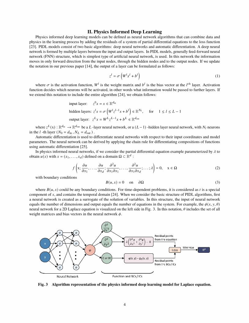
a neural network is created as a surrogate of the solution of variables. In this structure, the input of neural network

equals the number of dimensions and output equals the number of equations in the system. For example, the q(G, H, \)

neural network for a 2D Laplace equation is visualized on the left side in Fig. 3. In this notation, \ includes the set of all

weight matrices and bias vectors in the neural network q.

Fig. 3 Algorithm representation of the physics informed deep learning model for Laplace equation.

4

In the second part of the algorithm, the q neural network is limited to provide physics enforced by equations,

boundary conditions, and initial conditions. In order to achieve this, initial data distribution in the domain is provided

with various approaches. These points are named as residual points and can be distributed by mathematically or

randomly. Residual points consist of the data from the equation and the boundary/initial conditions, so they form the

physics informed part of algorithm shown on the right side in Fig. 3. Then, the loss function is defined to monitor the

variation between the neural network and the constraints as the weighted summation of the !2 norm of residuals for the

equation and boundary/initial conditions.

! (\; ') = F 5 ! 5

(

\; ' 5

)

+ F1!1 (\; '1) (4)

where ' 5 and '1 are the residual points, and F 5 and F1 are the weights of functions and boundary/initial conditions,

respectively. ! 5 and !1 can be defined as

! 5

(

\; ' 5

)

=1

�

�' 5

�

�

∑

x∈' 5

5

(

x;mD̂

mG1

, . . . ,mD̂

mG3;

m2D̂

mG1mG1

, . . . ,m2D̂

mG1mG3; . . . ;_

)

2

2

(5a)

!1 (\; '1) =1

|'1 |

∑

x∈'1

‖�(D̂, x)‖22

(5b)

In the last step, the loss is tried to be minimized using the training algorithm. The most important point of getting

results from PDE using deep learning is constrain the neural network to minimize the PDE residual [24]. In training

phase there are two options: grid and stochastic training. Briefly, while grid training initialize points on a lattice and

never change them during the training process, in stochastic training randomly the subset of points from a full training

set are selected in each optimization iteration [26].

III. Applications of the ModelIn this section, the results of several test applications of the physics informed neural network model are presented

to show its applicability, limits, advantages, and disadvantages. The outcomes of these examples are compared with

validation data obtained either analytically or numerically.

In these applications, PIDL models generated using Julia programming language were examined in terms of possible

benefits and drawbacks. The basic library used to create algorithms, NeuralPDE.jl, can be described as a solver package

which consists of neural network solvers for partial equations using scientific machine learning (SciML) techniques

[27]. This package uses deep neural networks to solve high-dimensional PDEs with greatly increased generality in

addition to a remarkably decreased cost compared to conventional methods. Using the DiffEqFlux.jl package, it is

possible to add differential equation layers to neural networks using a range of differential equations models that allow

the use of a complete library of highly tested and optimized methods within neural networks [28]. Finally, the PDEs are

described using ModelingToolkit.jl, which is a modeling language for high-performance symbolic-numeric computation

in scientific computing and scientific machine learning [26]. This allows users to give a high-level description of a

model for symbolic pre-processing to analyze and enhance the model.

A. 2D Laplace Equation

In this application, a validation study is performed on the Laplace equation, which is well-known PDE example that

generally describes behavior of fluid potentials. In the problem Laplace equation on a domain [0,1] x [0,1] is given by

with the Drichlet boundary conditions.

m2k

mG2+m2k

mH2= 0 (6)

Boundary conditions are given as follows:

k(G, 0) = 0 (7a)

k(G, 1) = (G − G2) (7b)

k(0, H) = 0 (7c)

k(1, H) = 0 (7d)

5

The algorithm in Fig. 3 was generated by transferring the Laplace equation and boundary conditions to the PIDL

model as mentioned in the previous section. The parameters used in creating the model are summarized in Table 2.

Table 2 Parameters for the PIDL algorithm of the Laplace equation.

Parameters Values

Number of Dense Layers 3

Neurons in the 1BC 16

Neurons in the 2=3 16

Neurons in the 3A3 16

Activation function Identity

x-Domain [0.0, 1.0]

y-Domain [0.0, 1.0]

Discretization (dx, dy) (0.02, 0.02)

Training strategy Grid

Optimizer BFGS

Max. iteration 2000

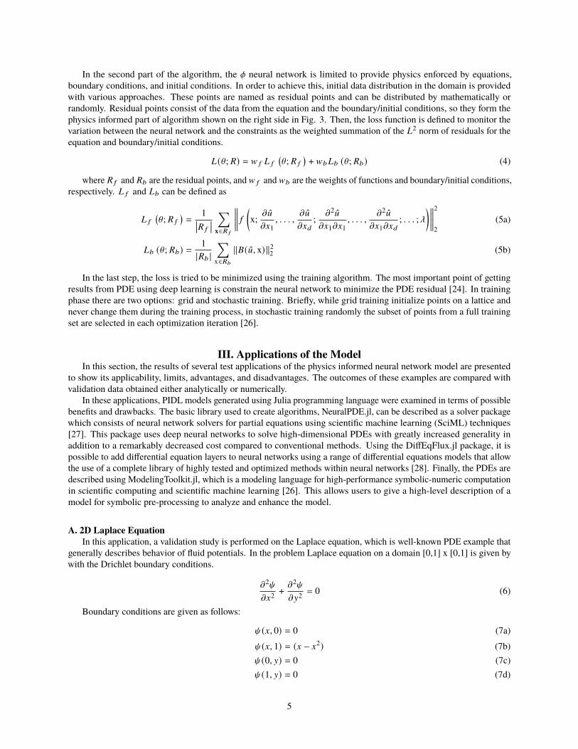
Moreover, the loss plot of the model is shown in Fig. 4. As can be seen from the figure, order of magnitude of the

loss value is between 10−5 and 10−6. This value can be further reduced with longer training processes.

Fig. 4 Loss curve of developed model for Laplace equation.

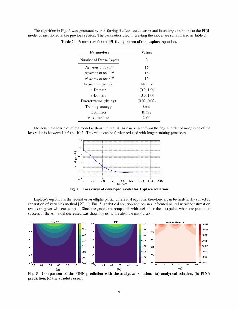
Laplace’s equation is the second-order elliptic partial differential equation; therefore, it can be analytically solved by

separation of variables method [29]. In Fig. 5, analytical solution and physics informed neural network estimation

results are given with contour plot. Since the graphs are compatible with each other, the data points where the prediction

success of the AI model decreased was shown by using the absolute error graph.

(a) (b) (c)

Fig. 5 Comparison of the PINN prediction with the analytical solution: (a) analytical solution, (b) PINN

prediction, (c) the absolute error.

6

In this application, no further action was used to improve the results. From this point of view, in the general

operations using the available automatic libraries, it is seen that there are errors in local points close to the boundary,

where the gradient is high. However, it is possible to reduce these errors with a better sampling or a longer training

process.

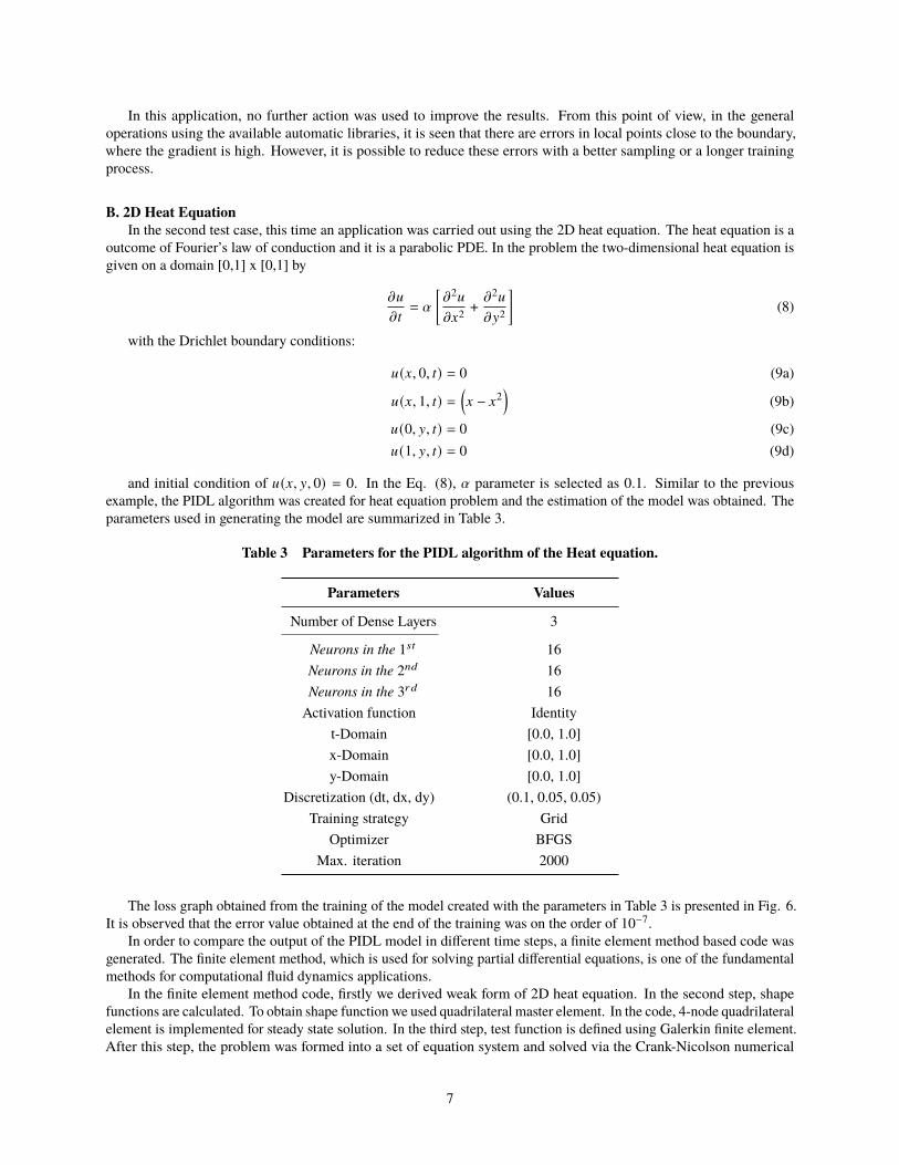
B. 2D Heat Equation

In the second test case, this time an application was carried out using the 2D heat equation. The heat equation is a

outcome of Fourier’s law of conduction and it is a parabolic PDE. In the problem the two-dimensional heat equation is

given on a domain [0,1] x [0,1] by

mD

mC= U

[

m2D

mG2+m2D

mH2

]

(8)

with the Drichlet boundary conditions:

D(G, 0, C) = 0 (9a)

D(G, 1, C) =(

G − G2)

(9b)

D(0, H, C) = 0 (9c)

D(1, H, C) = 0 (9d)

and initial condition of D(G, H, 0) = 0. In the Eq. (8), U parameter is selected as 0.1. Similar to the previous

example, the PIDL algorithm was created for heat equation problem and the estimation of the model was obtained. The

parameters used in generating the model are summarized in Table 3.

Table 3 Parameters for the PIDL algorithm of the Heat equation.

Parameters Values

Number of Dense Layers 3

Neurons in the 1BC 16

Neurons in the 2=3 16

Neurons in the 3A3 16

Activation function Identity

t-Domain [0.0, 1.0]

x-Domain [0.0, 1.0]

y-Domain [0.0, 1.0]

Discretization (dt, dx, dy) (0.1, 0.05, 0.05)

Training strategy Grid

Optimizer BFGS

Max. iteration 2000

The loss graph obtained from the training of the model created with the parameters in Table 3 is presented in Fig. 6.

It is observed that the error value obtained at the end of the training was on the order of 10−7.

In order to compare the output of the PIDL model in different time steps, a finite element method based code was

generated. The finite element method, which is used for solving partial differential equations, is one of the fundamental

methods for computational fluid dynamics applications.

In the finite element method code, firstly we derived weak form of 2D heat equation. In the second step, shape

functions are calculated. To obtain shape function we used quadrilateral master element. In the code, 4-node quadrilateral

element is implemented for steady state solution. In the third step, test function is defined using Galerkin finite element.

After this step, the problem was formed into a set of equation system and solved via the Crank-Nicolson numerical

7

method, which is equal to average of the Euler implicit and explicit methods. Detailed information about these steps can

be found in any computational fluid dynamics textbook [30, 31].

Fig. 6 Loss curve of developed model for heat equation.

The results achieved for two different time values, C = 0.1 and C = 1.0, are demonstrated in Fig. 7 and Fig. 8,

respectively. As in the previous test case, each PINN prediction is compared with validation data and absolute errors are

calculated.

(a) (b) (c)

Fig. 7 Comparison of the PINN prediction with the numerical solution at C = 0.1: (a) FEM result, (b) PINN

prediction, (c) the absolute error.

As seen in Fig. 7c, error values increase in a few data near the walls. It seems possible to reduce the error at these

points with longer training processes. Figure 8 shows the distribution at a time value closer to the steady-state. When

the error graph is examined, there were differences at much lower values than the solution close the initial state.

(a) (b) (c)

Fig. 8 Comparison of the PINN prediction with the numerical solution at C = 1.0: (a) FEM result, (b) PINN

prediction, (c) the absolute error.

8

C. Boundary Layer Over a Semi-Infinite Flat Plate

In this example, boundary layer over a semi-infinite flat plate is investigated. The Navier-Stokes equation for

two-dimensional laminar flow can be transformed to a reduced form using scale analysis. In this approach, the order of

magnitude of each term in the governing equations is estimated to be able to drop small terms.

For the flow along a flat plate parallel to the stream velocity U, we assume no pressure gradient, so the continuity

and momentum equation in the x-direction for steady motion in the boundary layer can be simplified as:

mD

mG+mE

mH= 0 (10a)

DmD

mG+ E

mD

mH= a

m2D

mH2(10b)

The appropriate boundary conditions are respectively: due to the viscosity the no slip condition at the plate, at the

plate surface there is no flow across it, and at infinity (outside the boundary layer) there is free-stream velocity.

D(G, 0) = 0 (11a)

E(G, 0) = 0 (11b)

D(G,∞) = * (11c)

In this application free-stream velocity * = 10</B and kinematic viscosity a = 1.4G10−5<2/B values are selected.Finite-difference method (FDM), which is a numerical technique for solving differential equations by approximating

derivatives with finite differences, was used as validation data. The physics informed neural network parameters used in

generating the model are summarized in Table 4.

Table 4 Parameters for the PIDL algorithm of the Boundary layer problem.

Parameters Values

Number of Dense Layers 3

Neurons in the 1BC 12

Neurons in the 2=3 12

Neurons in the 3A3 12

Activation function Identity

x-Domain [0.0, 1.0]

y-Domain [0.0, 0.02]

Discretization (dx, dy) (0.05, 0.001)

Training strategy Grid

Optimizer BFGS

Max. iteration 2500

The loss converged a value after nearly 2500 iterations; therefore, no more training is required for this problem.

Figure 9 shows the loss curve behavior in training phase.

Fig. 9 Loss curve of developed model for Boundary layer problem.

9

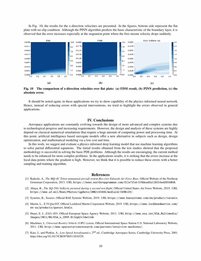
In Fig. 10, the results for the x-direction velocities are presented. In the figures, bottom side represent the flat

plate with no-slip condition. Although the PINN algorithm predicts the basic characteristic of the boundary layer, it is

observed that the error increases especially at the stagnation point where the free-stream velocity drops suddenly.

(a) (b) (c)

Fig. 10 The comparison of x-direction velocities over flat plate: (a) FDM result, (b) PINN prediction, (c) the

absolute error.

It should be noted again, in these applications we try to show capability of the physics informed neural network.

Hence, instead of reducing errors with special interventions, we tried to highlight the errors observed in general

applications.

IV. ConclusionsAerospace applications are constantly evolving towards the design of more advanced and complex systems due

to technological progress and increasing requirements. However, the design and analysis of these systems are highly

depend on classical numerical simulations that require a huge amount of computing power and processing time. At

this point, artificial intelligence based surrogate models offer a new alternative in subjects such as design, design

optimization, and mathematical modeling via a low cost and time.

In this work, we suggest and evaluate a physics informed deep learning model that use machine learning algorithms

to solve partial differential equations. The initial results obtained from the test studies showed that the proposed

methodology is successful in solving the basic PDE problems. Although the results are encouraging, the current method

needs to be enhanced for more complex problems. In the applications results, it is striking that the errors increase at the

local data points where the gradient is high. However, we think that it is possible to reduce these errors with a better

sampling and training algorithm.

References[1] Radecki, A., The MQ-4C Triton unmanned aircraft system flies over Edwards Air Force Base, Official Website of the Northrop

Grumman Corporation, 2013. URL https://news.northropgrumman.com/file?fid=578deadfa138354edf856048.

[2] Abaya, R., The XQ-58A Valkyrie pictured during a second test flight, Official United States Air Force Website, 2019. URL

https://www.af.mil/News/Photos/igphoto/2002145846/mediaid/3490129/.

[3] Systems, B., Taranis, Official BAE Systems Website, 2019. URL https://www.baesystems.com/en/product/taranis.

[4] Martin, L., X-59 QueSST, Official Lockheed Martin Corporation Website, 2019. URL https://www.lockheedmartin.com/

en-us/products/quesst.htmls.

[5] Huart, E. J., ESA’s IXV, Official European Space Agency Website, 2011. URL http://www.esa.int/ESA_Multimedia/

Images/2011/06/ESA_s_IXV#.Xt3xgQJc5Awlink.

[6] Machines, I., Universal Reentry Vehicle (URV) system, Official International Space Station U.S. National Laboratory Website,

2011. URL http://www.spacestationresearch.com/partner/intuitive-machines/.

[7] Katz, J., and Plotkin, A., Low-Speed Aerodynamics, 2nd ed., Cambridge Aerospace Series, Cambridge University Press, 2001.

https://doi.org/10.1017/CBO9780511810329.

10

[8] Cummings, R. M., Mason, W. H., Morton, S. A., and McDaniel, D. R., Applied Computational Aerodynamics: A

Modern Engineering Approach, Cambridge Aerospace Series, Cambridge University Press, 2015. https://doi.org/10.1017/

CBO9781107284166.

[9] Karali, H., Yukselen, M. A., and Inalhan, G., “A New Non-Linear Lifting Line Method for 3D Analysis of Wing/Configuration

Aerodynamic Characteristics with Application to UAVs,” AIAA Scitech 2019 Forum, San Diego, CA, 2019, p. 2119.

https://doi.org/10.2514/6.2019-2119.

[10] Slotnick, J., Khodadoust, A., Alonso, J., Darmofal, D., Gropp, W., Lurie, E., and Mavriplis, D., “CFD vision 2030 study: a path

to revolutionary computational aerosciences,” Nasa technical report, NASA Langley Research Center, Hampton, VA, United

States, 2014. URL https://ntrs.nasa.gov/search.jsp?R=20140003093.

[11] Spalart, P., “Strategies for turbulence modelling and simulations,” International Journal of Heat and Fluid Flow, Vol. 21, 2000,

pp. 252–263. https://doi.org/10.1016/S0142-727X(00)00007-2.

[12] Pezzella, G., and Viviani, A., “Aerodynamic performance analysis of a winged re-entry vehicle from hypersonic down to

subsonic speed,” Aerospace Science and Technology, Vol. 52, 2016, pp. 129–143. https://doi.org/10.1016/j.ast.2016.02.030.

[13] Brunton, S. L., Noack, B. R., and Koumoutsakos, P., “Machine Learning for Fluid Mechanics,” Annual Review of Fluid

Mechanics, Vol. 52, No. 1, 2020, pp. 477–508. https://doi.org/10.1146/annurev-fluid-010719-060214.

[14] Karali, H., Demirezen, M. U., Yukselen, M. A., and Inalhan, G., “Design of a Deep Learning Based Nonlinear Aerodynamic

Surrogate Model for UAVs,” AIAA Scitech 2020 Forum, Orlando, FL, 2020, p. 1288. https://doi.org/10.2514/6.2020-1288.

[15] Obiols-Sales, O., Vishnu, A., Malaya, N., and Chandramowlishwaran, A., “CFDNet: a deep learning-based accelerator for fluid

simulations,” arXiv preprint arXiv:2005.04485, 2020.

[16] Ranade, R., Hill, C., and Pathak, J., “DiscretizationNet: A Machine-Learning based solver for Navier-Stokes Equations using

Finite Volume Discretization,” , 2020.

[17] Raissi, M., Perdikaris, P., and Karniadakis, G. E., “Physics Informed Deep Learning (Part I): Data-driven Solutions of Nonlinear

Partial Differential Equations,” , 2017.

[18] Raissi, M., Perdikaris, P., and Karniadakis, G. E., “Physics Informed Deep Learning (Part II): Data-driven Discovery of

Nonlinear Partial Differential Equations,” , 2017.

[19] Sun, L., Gao, H., Pan, S., and Wang, J.-X., “Surrogate modeling for fluid flows based on physics-constrained deep

learning without simulation data,” Computer Methods in Applied Mechanics and Engineering, Vol. 361, 2020, p. 112732.

https://doi.org/10.1016/j.cma.2019.112732.

[20] Zhu, Y., Zabaras, N., Koutsourelakis, P.-S., and Perdikaris, P., “Physics-constrained deep learning for high-dimensional

surrogate modeling and uncertainty quantification without labeled data,” Journal of Computational Physics, Vol. 394, 2019, pp.

56 – 81. https://doi.org/10.1016/j.jcp.2019.05.024.

[21] Raissi, M., Perdikaris, P., and Karniadakis, G., “Physics-informed neural networks: A deep learning framework for solving

forward and inverse problems involving nonlinear partial differential equations,” Journal of Computational Physics, Vol. 378,

2019, pp. 686 – 707. https://doi.org/10.1016/j.jcp.2018.10.045.

[22] Rao, C., Sun, H., and Liu, Y., “Physics-informed deep learning for incompressible laminar flows,” Theoretical and Applied

Mechanics Letters, Vol. 10, No. 3, 2020, pp. 207 – 212. https://doi.org/10.1016/j.taml.2020.01.039.

[23] Shukla, K., Di Leoni, P. C., Blackshire, J., Sparkman, D., and Karniadakis, G. E., “Physics-Informed Neural Network for

Ultrasound Nondestructive Quantification of Surface Breaking Cracks,” Journal of Nondestructive Evaluation, Vol. 39, No. 61,

2020. https://doi.org/10.1007/s10921-020-00705-1.

[24] Lu, L., Meng, X., Mao, Z., and Karniadakis, G. E., “DeepXDE: A deep learning library for solving differential equations,”

CoRR, Vol. abs/1907.04502, 2019. URL http://arxiv.org/abs/1907.04502.

[25] Baydin, A. G., Pearlmutter, B. A., Radul, A. A., and Siskind, J. M., “Automatic Differentiation in Machine Learning: A Survey,”

J. Mach. Learn. Res., Vol. 18, No. 1, 2017, p. 5595–5637.

[26] Zubov, K., “Physics-informed neural networks (PINNs) solver on Julia,” , 2020. URL https://nextjournal.com/kirill_zubov/

physics-informed-neural-networks-pinns-solver-on-julia-gsoc-2020-final-report.

11

[27] Rackauckas, C., and Nie, Q., “DifferentialEquations.jl – A Performant and Feature-Rich Ecosystem for Solving Differential

Equations in Julia,” The Journal of Open Research Software, Vol. 5, No. 1, 2017. https://doi.org/10.5334/jors.151.

[28] Rackauckas, C., Innes, M., Ma, Y., Bettencourt, J., White, L., and Dixit, V., “Diffeqflux.jl-A julia library for neural differential

equations,” arXiv preprint arXiv:1902.02376, 2019.

[29] Friedman, N., Lecture notes in Analytical solution of ODEs and PDEs, Technische Universitat Braunschweig, 2015.

[30] Reddy, J., and Gartling, D., The Finite Element Method in Heat Transfer and Fluid Dynamics, Applied and Computational

Mechanics, CRC Press, 2010.

[31] Hoffmann, K., and Chiang, S., Computational Fluid Dynamics, No. 1. c. in Computational Fluid Dynamics, Engineering

Education System, 2000.

12