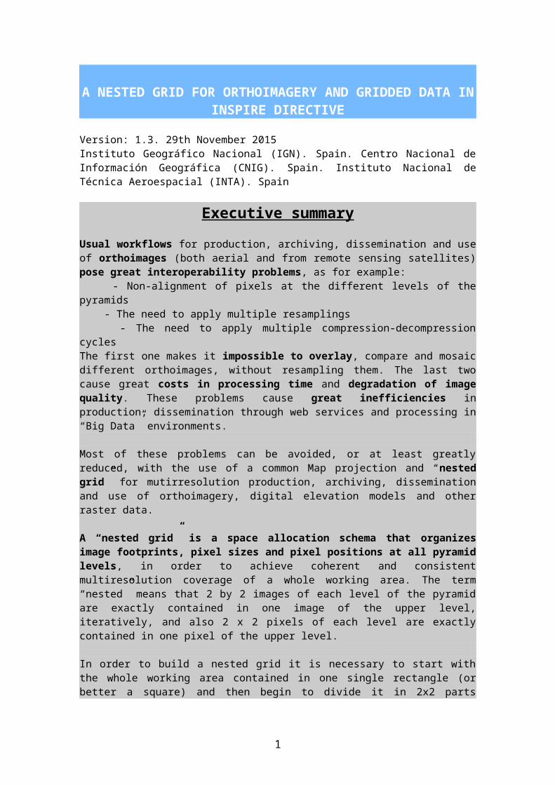
A NESTED GRID FOR ORTHOIMAGERY AND GRIDDED DATA IN INSPIRE DIRECTIVE

Version: 1.3. 29th November 2015Instituto Geográfico Nacional (IGN). Spain. Centro Nacional de Información Geográfica (CNIG). Spain. Instituto Nacional de Técnica Aeroespacial (INTA). Spain

Executive summary

Usual workflows for production, archiving, dissemination and use of orthoimages (both aerial and from remote sensing satellites) pose great interoperability problems, as for example: - Non-alignment of pixels at the different levels of the pyramids - The need to apply multiple resamplings - The need to apply multiple compression-decompression cyclesThe first one makes it impossible to overlay, compare and mosaic different orthoimages, without resampling them. The last two cause great costs in processing time and degradation of image quality. These problems cause great inefficiencies in production, dissemination through web services and processing in “Big Data” environments.

Most of these problems can be avoided, or at least greatly reduced, with the use of a common Map projection and “nested grid” for mutirresolution production, archiving, dissemination and use of orthoimagery, digital elevation models and other raster data.

A “nested grid” is a space allocation schema that organizes image footprints, pixel sizes and pixel positions at all pyramid levels, in order to achieve coherent and consistent multiresolution coverage of a whole working area. The term “nested” means that 2 by 2 images of each level of the pyramid are exactly contained in one image of the upper level, iteratively, and also 2 x 2 pixels of each level are exactly contained in one pixel of the upper level.

In order to build a nested grid it is necessary to start with the whole working area contained in one single rectangle (or better a square) and then begin to divide it in 2x2 parts iteratively. Such “nested grid” must be complemented by an appropriate “tiling schema” based on the “quad-tree” concepts.

In the last years a “de facto” standard Map Projection and Tiling Schema has emerged and has been adopted by virtually all major geospatial data providers, as Google Maps, Bing Maps, OpenStreetMap, Mapquest, Mapbox, and many others. It has also been adopted in OGC “WMTS Simple Profile” (WMTS-SP) and approved recently as official standard. WMTS-SP defines a suitable Map Projection (Web Mercator, EPSG:3857) and a tiling schema that is in fact a nested grid.

In this document we propose the use of this tiling schema as common nested grid for orthoimagery, DEMs and other types of raster data. The use of this nested grid constitutes the solution to most of the interoperability problems that both producers and users of these types of data suffer every day.

Also, a proposal is made for the implementation of some options of TIFF format (Tiled, Pyramidal, JPEG compressed and BigTIFF) to solve the problems posed by the enormous number of tiny JPEG tiles needed by WMTS services.

In order to adopt the proposed nested grid and TIFF options, some minor but important changes must be made to Inspire Data Specifications on Orthoimagery, Elevations, Coordinate Reference Systems and Geographical Grid Systems.

1

Index

Executive summary

1. Motivation2. Problems of current workflows for aerial orthophoto

- Nonaligned pixels at certain pyramid levels- Empty wedges- Images in different Zones of the map projections- Multiple compressions and decompressions- Multiple versions stored

3. Problems of current workflows for satellite Remote Sensing- Nonaligned pixels at certain pyramid levels- Images in different Zones of the map projection

The apparent solution of nearest neighbor resampling- Geographic projection problems

4. Requirements for an optimal workflow- Avoid the use of Map Projections with different zones.- Avoid repeated resampling. - Pixel borders should be aligned at all levels of the pyramid- Avoid “empty wedges”- Avoid repeated compression and decompression

5. The solution: a Nested GridWhat is a nested grid?

6. Geographic projection versus Mercator projectionWeb MercatorThe whole Earth in a single pixel

7. The quadtree structure- Pixel alignment at all pyramid levels- Open source libraries support- Coherence with JPEG blocks

8. SuperTiles and BigTiles9. Tiled TIFF as container of tiles

- JPEG compressed TIFF- All tiles pre-generated- Big TIFF- Pyramidal TIFF

10. Some additional issues- Use the scale factor- Secant Mercator Projection- The advantages of integer pixel sizes- 254 dpi as reference screen resolution

11. Application to Digital Elevation Models12. Application to raster maps

Annex 1: Proposals to INSPIRE Data SpecificationsAnnex 2: Quadtree tile naming schema

2

1. Motivation

INSPIRE Orthoimagery theme includes two main different types of data with slightly different needs:

- Aerial orthophotos: the main needs being efficient data production and storage, fast and flexible multiscale visualization and overlay with light web clients or desktop GIS programs through Internet (WMS, WMTS or WCS services), together with the maximum preservation of original image quality.

- Satellite orthoimages for remote sensing: the main needs are quick processing of massive amounts of data (the so-called “Big Data” problem) for multitemporal and multiscale analysis, integration of data from multiple satellites, quasi-real time processing and information dissemination, together with the maximum preservation of original radiometric values.

In this document we propose the use of WMTS Simple Profile map projection and tiling tchema as unique nested grid for the production, storage, reprocessing and dissemination of both kinds of ortohoimagery and also for other raster data, such as Digital Elevation Models (DEM), biophysical parameters, etc.

In order to understand the need of this proposal, and why it is the most feasible solution to the interoperability problems that we suffer every day, the reader should take the time to go through the following pages

2. Problems of current workflows for aerial orthophotos

Present workflows in aerial orthophoto production, storage and dissemination normally include the following steps:

1) Produce uncompressed orthophotos, by mosaicking several orthorectified aerial images in “production units” (normally called “sheets” for historical reasons). These “sheets” are rectangles that can be generated and stored in one single uncompressed image file (e.g: a single GeoTIFF file).1

2) Mosaic several uncompressed orthophotos in one larger compressed image file (e.g: in JPEG2000 format) in order to facilitate management and dissemination, by reducing the number of files2.

3) Set up WMS and WCS services, serving these compressed mosaics.

4) Produce JPEG tiles for WMTS services: millions of small JPEG images must be produced (either pre-cached or “on the fly”) in one or several projections.

5) Set up WMTS serving these tiles.

1 In INSPIRE Specifications, one production unit, called AggregatedMosaicElement is composed by several individual orthophotos coming from each one for a single photograph, called SingleMosaicElements

2 In INSPIRE Specifications several OrthoimageCoverages compose one OrthoimageAggregation

3

6) User connects to this Web services through a light web client or through a complete desktop GIS program.

This workflow generates the following problems:

Problem 1: Nonaligned pixels at certain pyramid levelsIn most cases the production units (or “sheets”) are inherited from traditional topographic maps. These are usually rectangles in geographical units. But in frequently used cartographic projections, such as UTM, these map sheets are not rectangular: instead they become irregular quadrilaterals, and not oriented to the North. So we are obliged to extend the orthoimages to the map sheet’s bounding box (Figure 1). This causes overlaps between adjacent sheets which increases file sizes and causes other problems as we will see after.

Figure 1: The footprint of a map sheet in UTM projection (green) and the bounding box needed to obtain rectangular images (blue). The choice of a sheet division that is not rectangular nor

oriented to the north in the map projection causes problems afterwards.

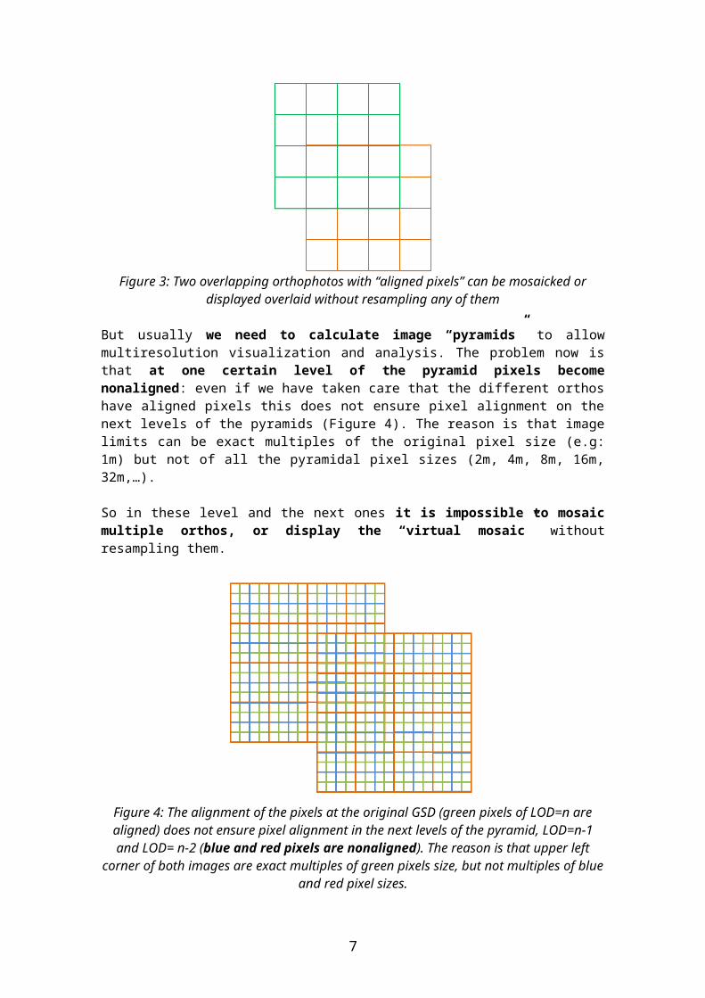
If we take the strict bounding rectangles as limits for the orthoimages, they will have “nonaligned” pixels (Figure 2), because in general the upper left corner of these orthoimages will not be multiple of pixel size. This makes it impossible to mosaic multiple orthophotos or even overlay them in a viewer without resampling them.

Figure 2: Two overlapping orthophotos with “nonaligned pixels” cannot be mosaicked or even displayed overlaid without resampling one of them

Resampling is computing demanding and causes image degradation, so we should “force” the alignment of the pixels by making (X, Y) coordinates of the “upper left corner of the upper left pixel” of all the orthos exact multiples of pixel size (Figure 3).

4

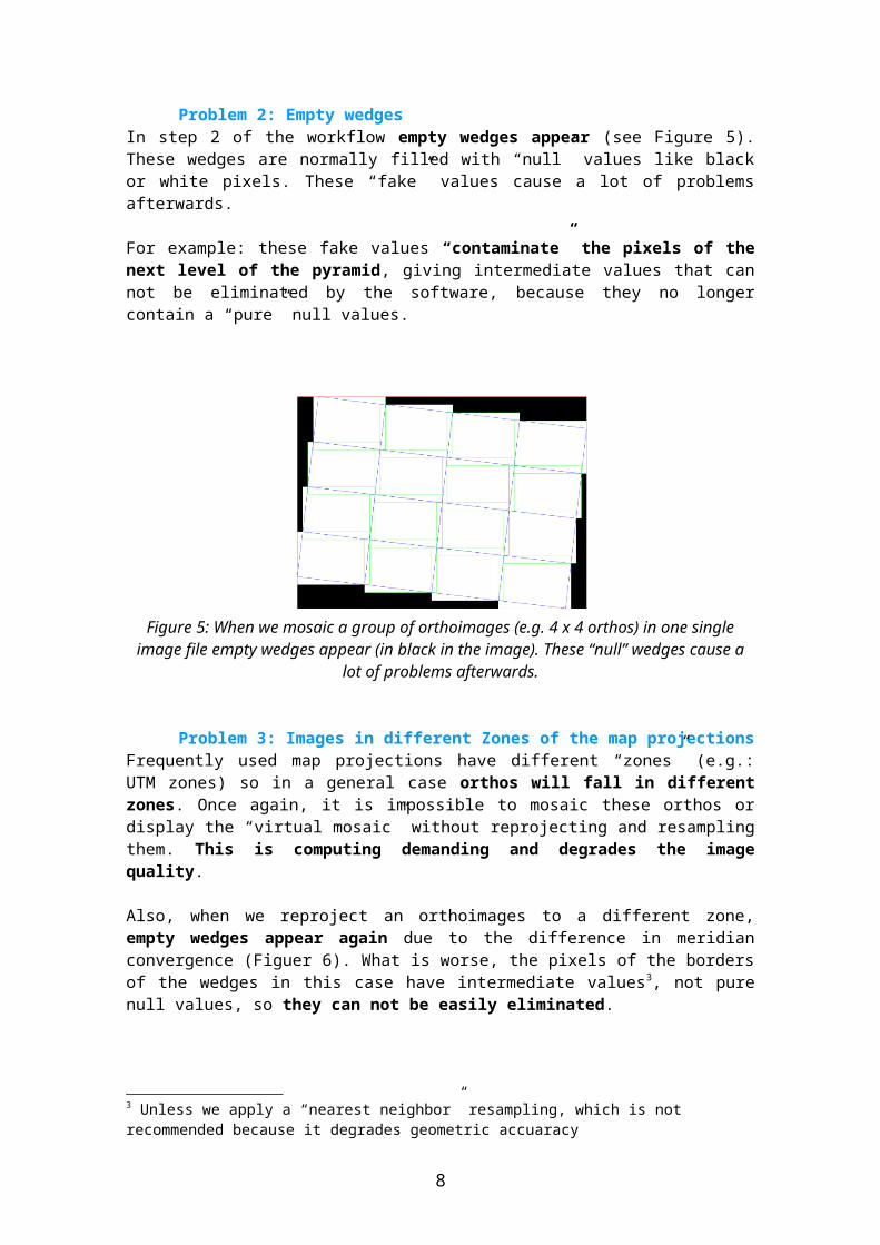
Figure 3: Two overlapping orthophotos with “aligned pixels” can be mosaicked or displayed overlaid without resampling any of them

But usually we need to calculate image “pyramids” to allow multiresolution visualization and analysis. The problem now is that at one certain level of the pyramid pixels become nonaligned: even if we have taken care that the different orthos have aligned pixels this does not ensure pixel alignment on the next levels of the pyramids (Figure 4). The reason is that image limits can be exact multiples of the original pixel size (e.g: 1m) but not of all the pyramidal pixel sizes (2m, 4m, 8m, 16m, 32m,…).

So in these level and the next ones it is impossible to mosaic multiple orthos, or display the “virtual mosaic” without resampling them.

Figure 4: The alignment of the pixels at the original GSD (green pixels of LOD=n are aligned) does not ensure pixel alignment in the next levels of the pyramid, LOD=n-1 and LOD= n-2

(blue and red pixels are nonaligned). The reason is that upper left corner of both images are exact multiples of green pixels size, but not multiples of blue and red pixel sizes.

Problem 2: Empty wedgesIn step 2 of the workflow empty wedges appear (see Figure 5). These wedges are normally filled with “null” values like black or white pixels. These “fake” values cause a lot of problems afterwards.

For example: these fake values “contaminate” the pixels of the next level of the pyramid, giving intermediate values that can not be eliminated by the software, because they no longer contain a “pure” null values.

5

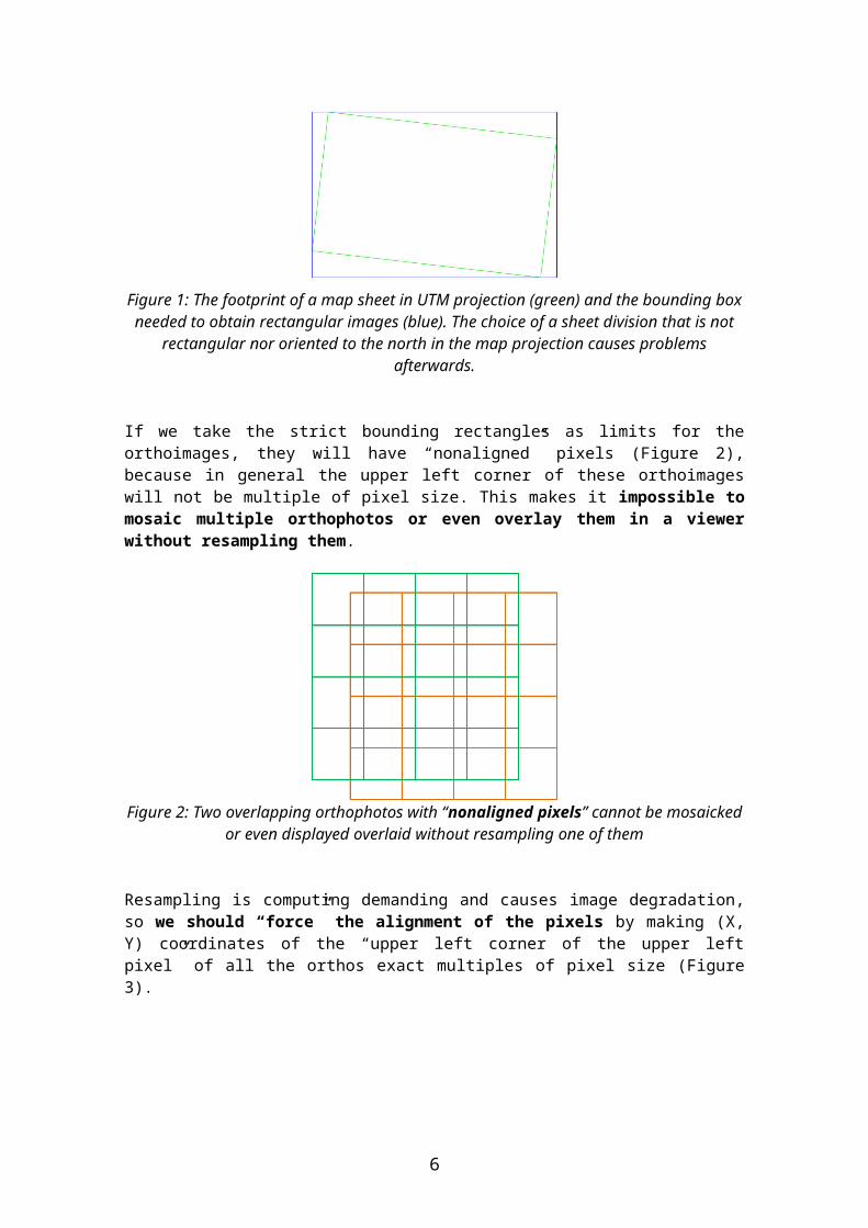
Figure 5: When we mosaic a group of orthoimages (e.g. 4 x 4 orthos) in one single image file empty wedges appear (in black in the image). These “null” wedges cause a lot of problems

afterwards.

Problem 3: Images in different Zones of the map projections Frequently used map projections have different “zones” (e.g.: UTM zones) so in a general case orthos will fall in different zones. Once again, it is impossible to mosaic these orthos or display the “virtual mosaic” without reprojecting and resampling them. This is computing demanding and degrades the image quality.

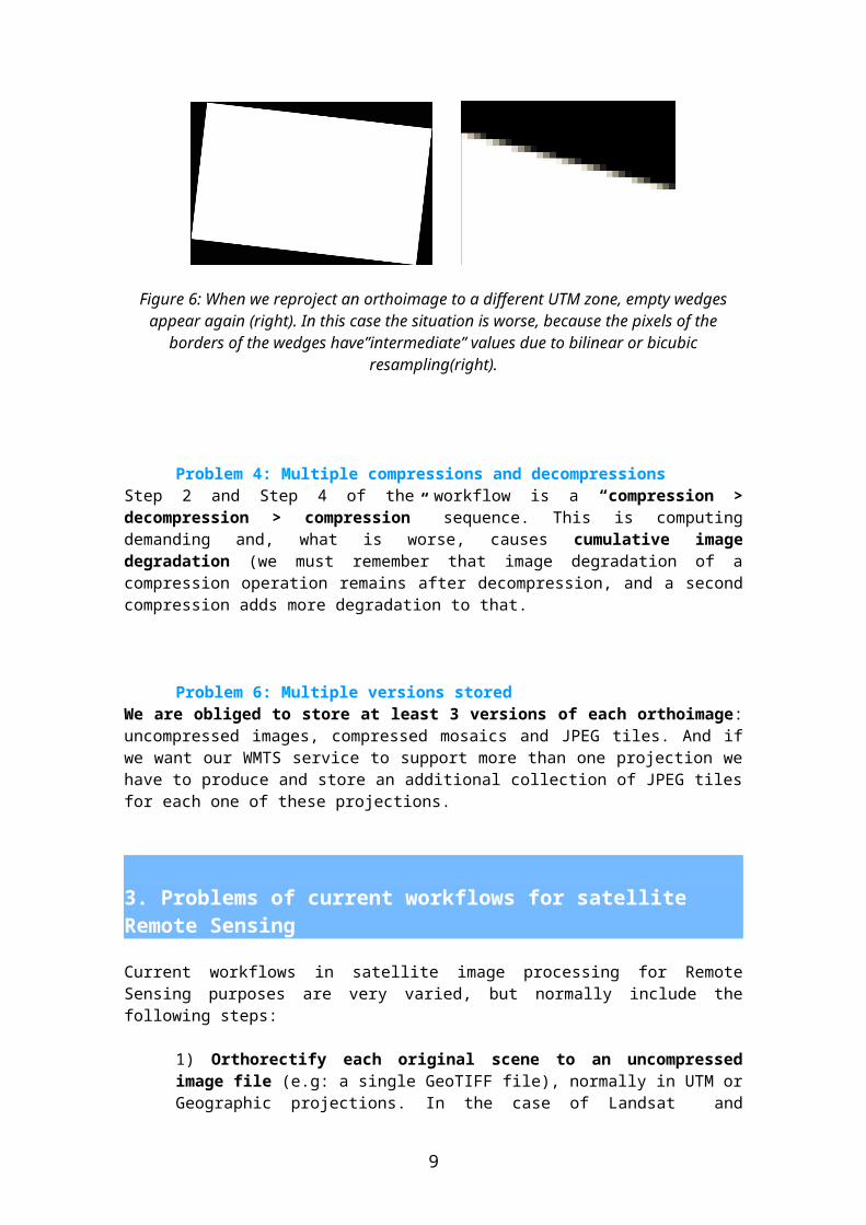
Also, when we reproject an orthoimages to a different zone, empty wedges appear again due to the difference in meridian convergence (Figuer 6). What is worse, the pixels of the borders of the wedges in this case have intermediate values3, not pure null values, so they can not be easily eliminated.

Figure 6: When we reproject an orthoimage to a different UTM zone, empty wedges appear again (right). In this case the situation is worse, because the pixels of the borders of the wedges

have”intermediate” values due to bilinear or bicubic resampling(right).

Problem 4: Multiple compressions and decompressionsStep 2 and Step 4 of the workflow is a “compression > decompression > compression” sequence. This is computing demanding and, what is worse, causes cumulative image degradation (we must remember that image degradation of a compression operation remains after decompression, and a second compression adds more degradation to that.

3 Unless we apply a “nearest neighbor” resampling, which is not recommended because it degrades geometric accuaracy

6

Problem 6: Multiple versions storedWe are obliged to store at least 3 versions of each orthoimage: uncompressed images, compressed mosaics and JPEG tiles. And if we want our WMTS service to support more than one projection we have to produce and store an additional collection of JPEG tiles for each one of these projections.

3. Problems of current workflows for satellite Remote Sensing

Current workflows in satellite image processing for Remote Sensing purposes are very varied, but normally include the following steps:

1) Orthorectify each original scene to an uncompressed image file (e.g: a single GeoTIFF file), normally in UTM or Geographic projections. In the case of Landsat and Sentinel 2 images, each scene is corrected in the UTM zone in which it has the biggest part.4

2) Perform radiometric corrections such as atmospheric correction, topographic correction, BRDF5 correction, etc.

3) Run complex algorithms to obtain biophysical parameters, land cover classifications, etc. These algorithms normally need to overlap, intercompare and mix radiometric data from images of different dates, mixing also other geographic information (Digital Elevation Models, training areas, LiDAR point clouds, in-situ sensors, etc). There is also an increasing tendency to mix data from different sensors with different GSD, bands, etc.

4) The output of these complex processes is generally a gridded dataset.

5) Set up WMS, WCS and WMTS services to serve the output datasets.

This workflow generates the following problems:

Problem 1: Nonaligned pixels at certain pyramid levels (same as for orthophotos)In remote sensing workflows we don’t normally mosaic images, but here pixel nonalignment makes it impossible to directly compare radiometric values for different dates without resampling them or introducing geometric displacements. This fact has very negative consequences in multitemporal analysis, change detection, etc. Resampling is computationally demanding and causes degradation of radiometric values so it should be avoided as much as possible.

Even if the original pixels are aligned, we would need that the pixels of other levels of the pyramid were also aligned, in order to perform multiresolution analysis. As we explained in the case of orthophotos, this is impossible for overlapping images (see figure 3).

Problem 2: Images in different Zones of the map projection

4 Today this task is normally routinely performed by the satellite operator.

5 BRDF: Bidirectional Reflectance Distribution Function

7

Step 3 implies the need to reproject and resample when we need to compare images in different UTM zones.

The apparent solution of nearest neighbor resamplingSome remote sensing scientists maintain that the solution to radiometric degradation when resampling is to perform “nearest neighbor” resampling, because it preserves the original radiometric values. This is a big mistake: nearest neighbor resampling introduces a displacement of the footprint of every pixel in the image6.

These geometric displacements should be avoided for many reasons, one of the most important being that leads to incorrect multitemporal analysis.

Problem 3: Geographic projection problemsWhen geographic projection is used to orthorectify the images, the problem is that it is not a conformal projection, so it does not maintain shapes: square pixels on the projection are rectangular on the ground, and have very high aspect ratios (length/width) at high latitudes. As much as 2.00 at 60º latitude and 5.75 at 80º latitude!

Conformal projections should be preferred in Remote Sensing because “directional isotropy” is supposed for some algorithms such as adjacency effect correction, filters, etc. This isotropy is not true for images in geographic projection.

Another side effect of high aspect ratios rectangular pixels that has not been well studied until now is how the shape of the pixels on the ground affects the visual and radiometric quality of the resampling made with traditional algorithms like bilinear or bicubic convolution, etc.

On the other hand pixels in Mercator projection are locally squares on the ground, so the images are locally isotropic.

Also, a conformal projection allows faster and easier calculation of sun directions for the algorithms that require it (e.g: topographic shadowing correction, etc.)

4. Requirements for an optimal workflow

After the explanation of the problems, the following requirements appear for an optimal workflow:

For orthophotos and satellite images:

1. Avoid the use of Map Projections with different zones.

2. Avoid repeated resampling. Ideally only one resampling should be performed during the whole process.

3. Pixel borders should be aligned at all levels of the pyramid

For orthophotos two additional requirements appear:

5. Avoid “empty wedges”. Production “sheets” should be rectangles in the map projection and oriented to the North. This would avoid all empty wedges appearance.

6 In average 0.25 pixels in X and Y each resampling

8

4. Avoid repeated compression and decompression. Ideally only one compression and one decompression should be performed during the whole process.

5. The solution: a Nested Grid

Both for aerial orhophotos and remote sensing images, the solution to the problems mentioned before resides in the use of a fixed and unique “nested grid” to produce, store, process, analyze, compare and serve orthoimages.

What is a nested grid?A “nested grid” is a “space allocation schema” that assures completely coherent and consistent multiresolution coverage of the whole working area with orthoimages by organizing image footprints, pixel sizes and pixel positions at all pyramid levels.

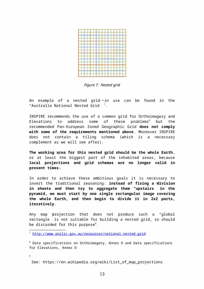
The term “nested” means that 2 by 2 images of each level of the pyramid are exactly contained in one image of the upper level, and also 2 x 2 pixels of each level are exactly contained in one pixel of the upper level, iteratively (Figure 7). This assures the alignment of pixels at all pyramid levels.

Figure 7: Nested grid

An example of a nested grid in use can be found in the “Australia National Nested Grid” 7.

INSPIRE recommends the use of a common grid for Orthoimagery and Elevations to address some of these problems8 but the recommended Pan-European Zoned Geographic Grid does not comply with some of the requirements mentioned above. Moreover INSPIRE does not contain a tiling schema (which is a necessary complement as we will see after).

The working area for this nested grid should be the whole Earth, or at least the biggest part of the inhabited areas, because local projections and grid schemas are no longer valid in present times.

In order to achieve these ambitious goals it is necessary to invert the traditional reasoning: instead of fixing a division in sheets and then try to aggregate them “upstairs” in the

7 http://www.anzlic.gov.au/resources/national_nested_grid

8 Data specifications on Orthoimagery, Annex D and Data specifications for Elevations, Annex D

9

pyramid, we must start by one single rectangular image covering the whole Earth, end then begin to divide it in 2x2 parts, iteratively.

Any map projection that does not produce such a “global rectangle” is not suitable for building a nested grid, so should be discarded for this purpose9.

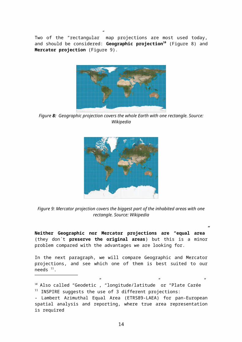
Two of the “rectangular” map projections are most used today, and should be considered: Geographic projection10 (Figure 8) and Mercator projection (Figure 9).

Figure 8: Geographic projection covers the whole Earth with one rectangle. Source: Wikipedia

Figure 9: Mercator projection covers the biggest part of the inhabited areas with one rectangle. Source: Wikipedia

Neither Geographic nor Mercator projections are “equal area” (they don´t preserve the original areas) but this is a minor problem compared with the advantages we are looking for.

In the next paragraph, we will compare Geographic and Mercator projections, and see which one of them is best suited to our needs 11.

9

See: https://en.wikipedia.org/wiki/List_of_map_projections

10 Also called “Geodetic”, “longitude/latitude” or “Plate Carée”11 INSPIRE suggests the use of 3 different projections:- Lambert Azimuthal Equal Area (ETRS89-LAEA) for pan-European spatial analysis and reporting, where true area representation is required- Lambert Conformal Conic (ETRS89-LCC) for conformal pan-European mapping at scales smaller than or equal to 1:500,000

10

6. Geographic projection versus Mercator projection

Geographic projection covers the whole Earth, but has a great disadvantage: it is not conformal.

For orthophotos it is very important to use a conformal projection in order to avoid strange appearance of common features like buildings, roundabouts, etc. and a “disagreeable perspective effect” in areas far of the equator (see Figure 10).

A Conformal projection is also useful in Remote Sensing, because it allows easy computation when dealing with directional effects such as BRDF correction, topographic shadows correction, etc. that are related with solar azimuth.

Mercator projection does not cover the whole Earth (a “cut” must be made at a certain latitude to avoid infinite coordinates), but it covers the biggest part of the inhabited areas. And it is conformal.

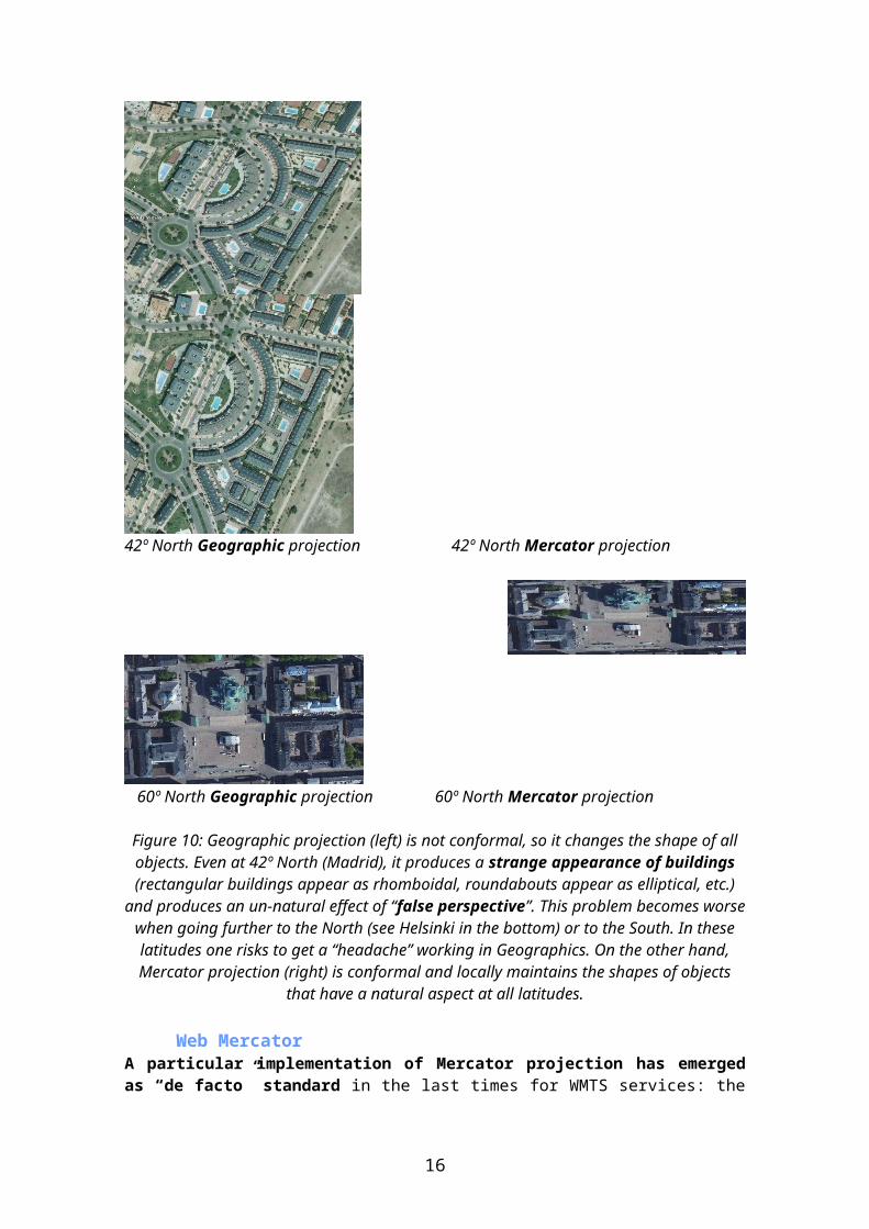
42º North Geographic projection 42º North Mercator projection

60º North Geographic projection 60º North Mercator projection

Figure 10: Geographic projection (left) is not conformal, so it changes the shape of all objects. Even at 42º North (Madrid), it produces a strange appearance of buildings (rectangular

buildings appear as rhomboidal, roundabouts appear as elliptical, etc.) and produces an un-natural effect of “false perspective”. This problem becomes worse when going further to the

North (see Helsinki in the bottom) or to the South. In these latitudes one risks to get a

- Transverse Mercator (ETRS89-TMzn) for conformal pan-European mapping at scales larger than 1:500,000.The problem is that none of them is able to display the whole Earth in a rectangular image, so none of them fits our purpose

11

“headache” working in Geographics. On the other hand, Mercator projection (right) is conformal and locally maintains the shapes of objects that have a natural aspect at all latitudes.

Web MercatorA particular implementation of Mercator projection has emerged as “de facto” standard in the last times for WMTS services: the “Spherical Mercator” or “Web Mercator” “almost-conformal” 12projection (EPSG:3857) used by Google Maps, Bing Maps, Yahoo Maps, Open Street Maps, ArcGIS Online13 and other geospatial data and API providers. It is associated to a Tiling Schema that is in fact a nested grid.

The advantages of this Web Mercator over other projections are described here: https://msdn.microsoft.com/en-us/library/bb259689.aspx

And also here: http://www.mapthematics.com/forums/viewtopic.php?f=8&t=251

Web Mercator and the associated Tiling Schema has recently become an official OGC standard (“WMTS Simple Profile14”).

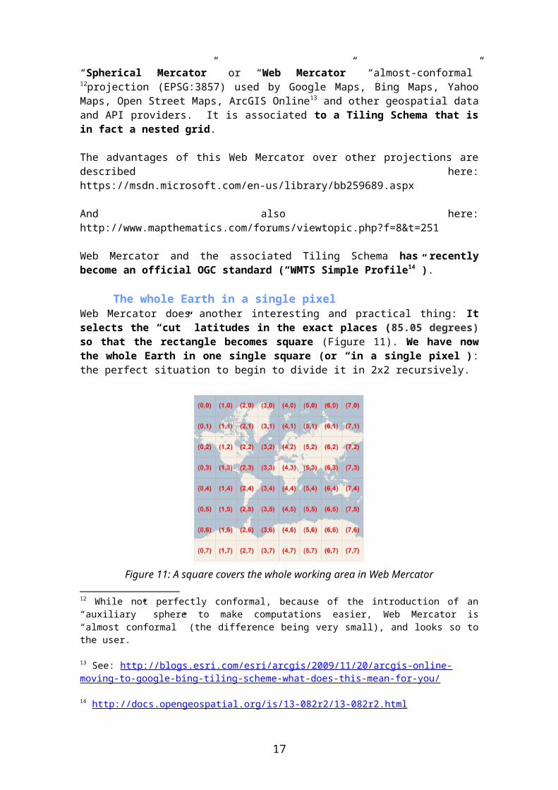
The whole Earth in a single pixelWeb Mercator does another interesting and practical thing: It selects the “cut” latitudes in the exact places (85.05 degrees) so that the rectangle becomes square (Figure 11). We have now the whole Earth in one single square (or “in a single pixel”): the perfect situation to begin to divide it in 2x2 recursively.

Figure 11: A square covers the whole working area in Web Mercator

7. The quadtree structure

12 While not perfectly conformal, because of the introduction of an “auxiliary” sphere to make computations easier, Web Mercator is “almost conformal” (the difference being very small), and looks so to the user.

13 See: http://blogs.esri.com/esri/arcgis/2009/11/20/arcgis-online-moving-to-google-bing-tiling-scheme-what-does-this-mean-for-you/

14 http://docs.opengeospatial.org/is/13-082r2/13-082r2.html

12

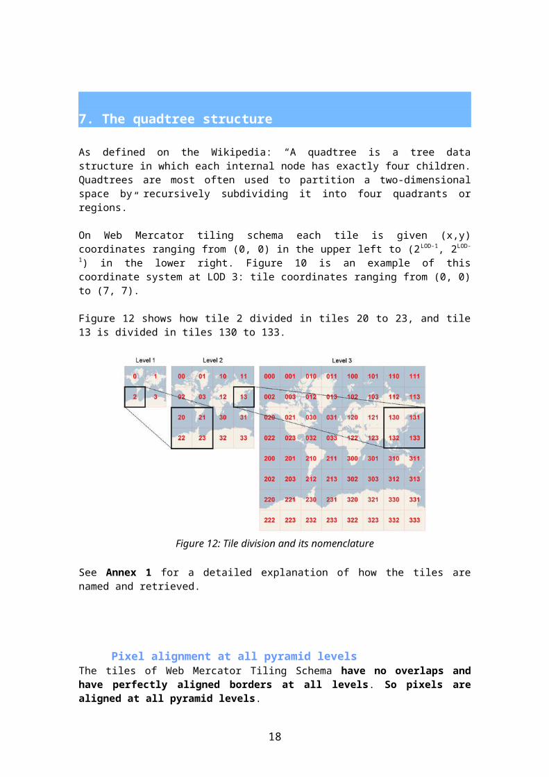
As defined on the Wikipedia: “A quadtree is a tree data structure in which each internal node has exactly four children. Quadtrees are most often used to partition a two-dimensional space by recursively subdividing it into four quadrants or regions.”

On Web Mercator tiling schema each tile is given (x,y) coordinates ranging from (0, 0) in the upper left to (2LOD-1, 2LOD-1) in the lower right. Figure 10 is an example of this coordinate system at LOD 3: tile coordinates ranging from (0, 0) to (7, 7).

Figure 12 shows how tile 2 divided in tiles 20 to 23, and tile 13 is divided in tiles 130 to 133.

Figure 12: Tile division and its nomenclature

See Annex 1 for a detailed explanation of how the tiles are named and retrieved.

Pixel alignment at all pyramid levelsThe tiles of Web Mercator Tiling Schema have no overlaps and have perfectly aligned borders at all levels. So pixels are aligned at all pyramid levels.

Open source libraries support“WMTS Simple Profile” grid and tiling schema is fully documented and supported by open source software libraries.

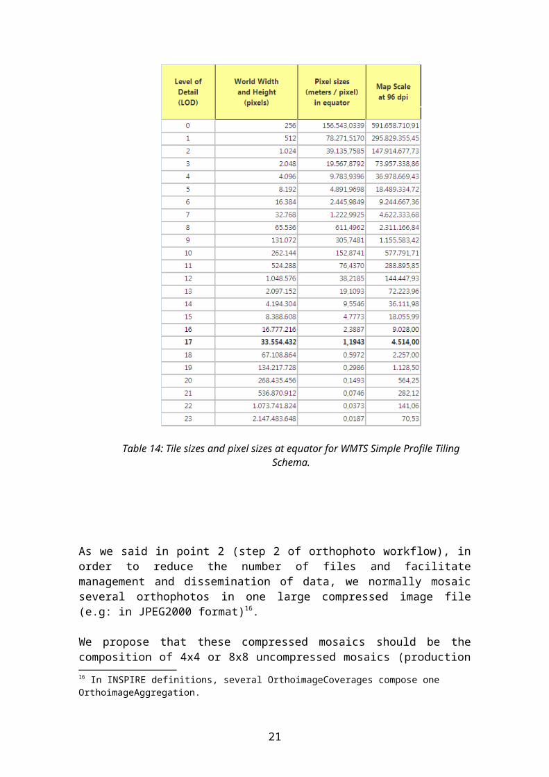
As we can see in Table 14, the tiling schema starts in LOD 0 (Level of Detail 0) covering the whole working area15 with one image of 256 x 256 pixels. Each time we increase zoom level (LOD), the pixel size divides by 2, and the number of pixels needed to cover the whole working area doubles.

The square images (called “tiles”) inside each level are always 256x256 pixels. The size of 256x256 is chosen to optimize the visualization speed (minimize the time to fill the screen with tiles) for WMTS services. These tiles are sent, compressed in JPEG, by the WMTS Server in response to each demand of the web client.

Coherence with JPEG blocks

15 The greatest part of inhabited areas (up to 85.05 degrees)

13

The size of 256 was also chosen because 256 is multiple of 8, and 8x8 is the “block” size of JPEG compression (figure 13). This is very important in order to minimize image degradation, as it assures that 32x32 JPEG “blocks” fit exactly in each tile, thus avoiding additional image degradation in possible subsequent mosaics due to the mix of “nonaligned” JPEG blocks.

Figure 13: JPEG compression blocks are 8x8 pixels that fitexactly inside each tile of 256x256 pixels

All these sizes (8, 256, etc…) are powers of 2 (2n) to allow “clean” pyramid building without border effects or surplus “orfan” pixels.

8. SuperTiles and BigTiles

But 256x256 tiles are way too small to be practical as “production units” (“sheets”) for uncompressed orthos, and even more for the compressed mosaics. So we propose to use as production units the same footprints of the Tiling Schema, but with a pixel size of other LOD.

For example: if we have LOD 14 pixel size and use LOD 8 tiles footprints as “production units”, they would be 16,384 x 16,384 pixels. This produces images of about 1 Gbyte (with 4 bands in 8 bits per band), adequate for uncompressed images. For short we will call these images “SuperTiles”.

Given the pixel size of the orthoimagery we want to produce, we can choose the SuperTile size that best suits our application simply by selecting the adequate footprint between the different LOD.

14

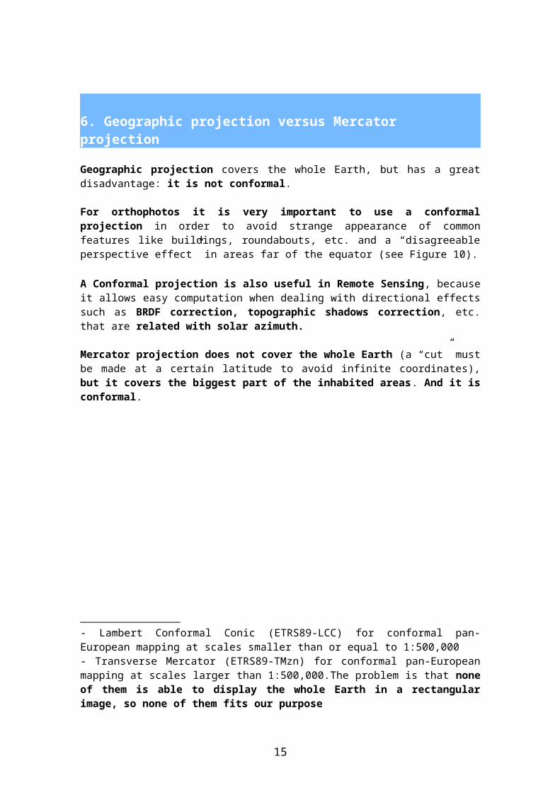
Table 14: Tile sizes and pixel sizes at equator for WMTS Simple Profile Tiling Schema.

As we said in point 2 (step 2 of orthophoto workflow), in order to reduce the number of files and facilitate management and dissemination of data, we normally mosaic several orthophotos in one large compressed image file (e.g: in JPEG2000 format)16.

We propose that these compressed mosaics should be the composition of 4x4 or 8x8 uncompressed mosaics (production units). For example: if we join and compress 8x8 uncompressed mosaics of 16,384x16,84 pixels, we obtain 131.072x131.072 compressed mosaics (approximately 6.8 Gbytes with 1:10 compression factor).

For short we will call these files “BigTiles”.

16 In INSPIRE definitions, several OrthoimageCoverages compose one OrthoimageAggregation.

15

9. Tiled TIFF as container of tiles

WMTS services require a huge number of tiles: hundreds of millions of individual “tiny” 256x256 JPEG files must be produced (either pre-cached or “on the fly”) in one or several “projections”17 These tiles are very difficult to manage in current computing environments, because operating systems are not prepared for such a large number of files. Even listing them can be a challenge, and if an operator needs to check them looking for problems or errors (corrupted tiles, missing tiles, etc.) he will discover it is absolutely impossible with such a huge number of files. (It is like “looking for a needle in a haystack”).

The solution is to store many tiny 256x256 tiles “inside” a bigger file. How this can be done, is explained now:

TIFF format has many options. One of them is called TiledTIFF. It was designed to allow quick access to any part of a big image without reading the whole file. TiledTIFF stores all the pixels in a tile together (while normal TIFF tiles store together all the pixels in a line)

When we generate a TiledTIFF we can choose the tile size. If we choose 256x256 tile size and the image size is a multiple of 256, the tiles we obtain inside the TiledTIFF are exactly the same tiles of an WMTS service. We only need to compress them in JPEG.

JPEG compressed TIFFBut another option of TIFF format is JPEG compression. It we generate a TiledTIFF with JPEG compression using the footprints and the pixel sizes Web Mercator Tiling Schema (of differents LOD as we saw before), we will end up with JPEG tiles inside the TiledTIFF that are exactly the same as the WMTS ready to be directly sent without the need to decompress and recompress them before sending,

With this approach we have two advantages at the same time:

1) We only compress once. So we save CPU time and preserve image quality2) We don not have to generate millions of individual 256x256 JPEG files. So we don’t fall in the directory burden.

This approach has already been implemented by Mapserver opensource project (see: http://mapserver.org/es/mapcache/caches.html#geo-tiff-caches):

“TIFF caches are the most recent addition to the family of cache types supported by MapCache (v.1.4). TIFF cache means that the TIFF file itself is used as the tile repository of a WMTS service. TIFF cache uses the internal tile structure of the TIFF specification to access tile data. Tiles can be stored in JPEG only (TIFF does not support PNG tiles).

As a single TIFF file may contain many tiles, there is a drastic reduction in the number of files that have to be stored on the file system, which solves the major shortcomings of the disk cache dealing with millions of files. Another advantage is that the same TIFF files can be used by programs or WMS servers that only understand regular GIS raster formats, and be served up with high performance for tile access.

The TIFF cache should be considered read-only for the time being. Write access is already possible but should be considered experimental as there might be some file corruption issues, notably on network file-systems. Note that until all the tiles in a given TIFF file have been seeded/created, the TIFF file is said to be “sparse” in the sense that it is missing a number of jpeg tiles. As such most non-GDAL based programs will have problems opening these incomplete files.

17 More rigorously: in one or several Spatial Reference Systems -SRS- defined by their EPSG code

16

Note that the TIFF tile structure must exactly match the structure of the grid used by the tileset, and the TIFF file names must follow strict naming rules”.

All tiles pre-generatedWe have to take into account that WMTS services performance advantage is based on the availability of “precached” tiles. Normally, we only “precache” 256x256 tiles until a certain LOD, because the work of generating them and the disk space to store JPEG files are so big, that it is not worth to pre-generate the LOD with smaller pixel sizes (the probability of being requested is lower than for tiles of bigger pixel sizes). So normally, for this big LODs we wait until the first request to generate this tiles “on the fly”, and then cache them for future requests. So user sees a decrease in performance.

On the other hand, the present proposal to use TiledTIFF with JPEG compression as the format for compressed mosaics, all the tiles, until the native resolution, are pregenerated, so there is no loss in performance at the biggest zoon levels.

Big TIFFTIFF files have a limitation of 4 Gbytes, due to 32 bit offsets. BigTIFF unofficial standard uses 64-bit offsets thereby supporting files up to 18,000 petabytes18. As BigTiles are usually bigger than 4 Gbytes, we must use BigTIFF format.

Pyramidal TIFFAnother interesting option of TIFF format is to contain image pyramids inside the same file. This option is very interesting for our purposes, because it allows fluent visualizations of big images in a desktop environment.

In conclusion: we propose to use these options off TIFF format:1) Geo: to provide georreference2) Big: to overcome the 4 GBytes limitation3) Tiled: to containWMTS tiles4) JPEG compression: to allow JPEG lossy compression (thus diminishing file size) and at the same time to serve WMTS tiles directly without the need to decompress and recompress them.5) Pyramidal: to accelerate visualization in desktop environments

10. Some additional issues

Some remaining issues should be addressed:

Issue 1: Mercator projection is not “equal area” nor “equidistant” as it has a different scale at each latitude. In other words, a fixed pixel size in the projection is in fact variable with latitude.

Issue 2: Pixel sizes (meters/pixel) in Table 14 are not integer, as we are used to.

Issue 3: Strange Map Scales. Map scales in Table 14 are not integer.

¿Can we find a solution for these issues?

18 http://www.awaresystems.be/imaging/tiff/faq.html

17

Solution to issue 1: Use the scale factorFor spatial analysis and reporting, where true area values are required, the solution is very simple: instead of counting pixels, take into account the real surface on the ground of each pixel (which is easily calculated using the “scale factor”).For visualization, the user has to get used to the fact that the scale is different at each latitude. This should not be a problem: sailors have done it for centuries, because Marine Charts always use Mercator projection.

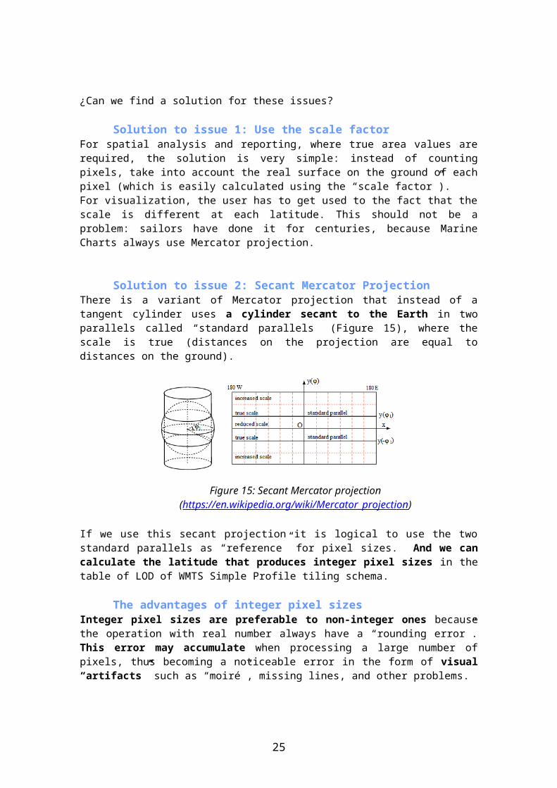
Solution to issue 2: Secant Mercator ProjectionThere is a variant of Mercator projection that instead of a tangent cylinder uses a cylinder secant to the Earth in two parallels called “standard parallels” (Figure 15), where the scale is true (distances on the projection are equal to distances on the ground).

Figure 15: Secant Mercator projection (https://en.wikipedia.org/wiki/Mercator_projection)

If we use this secant projection it is logical to use the two standard parallels as “reference” for pixel sizes. And we can calculate the latitude that produces integer pixel sizes in the table of LOD of WMTS Simple Profile tiling schema.

The advantages of integer pixel sizesInteger pixel sizes are preferable to non-integer ones because the operation with real number always have a “rounding error”. This error may accumulate when processing a large number of pixels, thus becoming a noticeable error in the form of visual “artifacts” such as “moiré”, missing lines, and other problems.

The latitude that produces integer pixel sizes happens to be 33.14489729º (see Table 15). So we should use a “Secant Mercator” projection with two standard parallels at 33.14489729º North and South.

In these 2 parallels pixel sizes (measured in meters) are integer up to LOD17. In centimeters, they are integer until LOD19, in mm until LOD20, and so on.

Solution to issue 3: 254 dpi as reference screen resolutionReal scale on a screen depends on the resolution (pixels per inch) of each screen. There is no obligation to use 96 dpi (dots per inch19) as a “reference” screen resolution (which produces ugly scale numbers even with “round” pixel sizes. As nowadays there exist a great variety of screen resolutions up to 400 dpi and more, we can choose one that produces “easy to remember” integer Map Scales. E.g: 10 pixels/mm = 254 dpi.

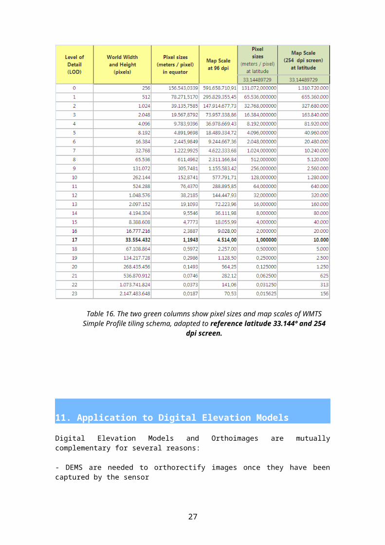
Now the LOD list looks much better (Table 16) with integer pixel sizes and integer Map scales.

19 dpi (dots per inch) is a slightly incorrect term. It should be “pixels per inch of screen”

18

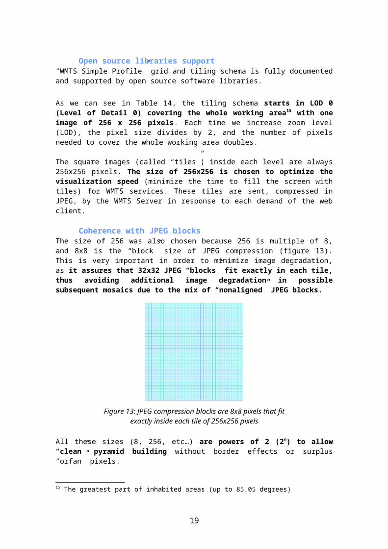
Table 16. The two green columns show pixel sizes and map scales of WMTS Simple Profile tiling schema, adapted to reference latitude 33.144º and 254 dpi screen.

11. Application to Digital Elevation Models

Digital Elevation Models and Orthoimages are mutually complementary for several reasons:

- DEMS are needed to orthorectify images once they have been captured by the sensor- DEMS are also needed to perform some radiometric corrections such as topographic shadows corrections- Orthoimages and DEMS can be combined to generate 3D (or 2.5 D) modeling- etc.

For these reasons, it is very important that we maximize the interoperability between both kinds of datasets. For this, it is imperative that they share a common grid and tiling schema.

19

Inspire Data Specification recognized this fact and for that reason included an Annex D describing this common grid both in Orthoimagery and in Elevation Data Themes. The problem is that, as we said before, the proposed Zoned Geographic Grid does not fulfill several of the requirements posed in this document for orthoimagey. Almost the same requirements are also applicable to Elevations, for analog reasons. This is the list of requirements, adapted to Elevation data:

1. Avoid the use of Map Projections with different zones.

2. Avoid repeated resampling. It is computing demanding and causes data degradation, so resampling should be avoided whenever possible. Ideally only one resampling should be performed during the whole process.

3. Samples should be aligned at all levels of the pyramid

5. Avoid “empty wedges”

For these reason, the Grid representation of Elevations should share the same nested grid as orthoimagery: Web Mercator Map Projection and Tiling Schema, as we have explained before.

There are only a few considerations that must be taken into account:

- Some algorithms use as input the Z coordinates of the center of orthoimagery pixels. E.g: orthorectification of an image using bicubic resampling, etc.

- Some other algorithms use as input the Z coordinates of the corners of orthoimagery pixels. E.g: topographic shadow correction, 2.5 D modeling by assigning color to the TIN triangles, orthorectification of an image using supersampling, etc.

So which option should we choose? Should we measure and store the Z of the corners of the grid or the Z of the centers of the squares of the grid?

Let’s take a common situation: We have a ~5m grid spacing DEM and we want to generate a 25 cm pixel size aerial orthophoto. We find these facts:

1) If we look to the green columns of Table 15, the first thing we see is that 5m is not a pixel size in the table. This is because all pixel sizes in the table are powers of 2 in these green columns. So if we want a complete coherence between ortho and DEM we should use a 4m DEM, instead of a 5m DEM. So the first advice is: choose a DEM sampling that is on the values of pixel sizes of the nested grid.

2) The second thing we see is that sample spacing of the DEM is much bigger than ortho pixel size: 4m versus 25cm is 16 times bigger. So if we need the Z of the centers of the orthoimage pixels as well as if we need the Z of the corners of the pixels, we are obliged to interpolate in both cases. The interpolation seems easier to perform starting with the corners of the pixels, but not anything very important.

3) The third consideration is pyramid consistency: if we have the Z of the center of the pixels in LOD = n (Figure 17 left), in order to generate LOD= n-1 we have to resample the heights (Figure 17 right) because there is no positional coincidence of the centers.

Resampling the heights produces a “degradation” of height values (loss of accuracy and appearance of artifacts) in the same way as a resampling an image produces a degradation of radiometric values. This need to resample the heights happens in all the

20

changes of LOD, so there is a cumulative degradation of height values when we go up the pyramid of LOD.

On the other hand, if we have the Z of the corners of the pixels in LOD = n (Figure 18 left), in order to generate LOD = n-1 we don’t need to interpolate (Figure 18 right) because there is positional coincidence of the corners.

Figure 17: In black: centers of blue pixels (LOD=n). In green: centers of red pixels (LOD=n-1). There is no coincidence between black and green points

Figure 18: In black: corners of blue pixels (LOD=n). In green: corners of red pixels (LOD=n-1). There is coincidence between black and green points

So, for this reason, and also because it seems a simpler schema easier to understand, and so less likely to produce mistakes, we recommend the second option: we should measure and store in the DEMs the corners of the nested grid, not the centers.

12. Application to raster maps

21

Raster maps can suffer the same problems than orthoimages and DEMS: loss of processing power, degradation of image quality, visual artifacts (due to black wedges and other problems), etc. These problems cause great inefficiencies in production, dissemination through web services and use from light web clients or desktop GIS programs. Also, they suffer the same problem with the big number of JPEG tiles that must be generated (either “precached” or on the fly) for a WMTS service.

We have to take into account that WMTS services performance advantage is based in the availability of “precached” tiles, with the pixels in the exact places. So if we need to overlay orthoimages, DEMs and raster maps in the same viewer, we will attain top visual performance only if we use the same map projection, pixel sizes and pixels positions for all layers being displayed, avoiding the use of any resampling.

For these reasons, the recommendation is to use for raster maps production and dissemination the same WMTS Simple Profile map projection (Web Mercator) and Tiling Schema, than for orthoimagery and DEMS.

In this way, a perfect coherence would be achieved for all these types of data.

22

Annex 1: Proposals to INSPIRE Data Specifications

In order to adopt the proposed nested grid and TIFF options, some minor but important changes must be made to Inspire Data Specifications, at least in Orthoimagery, Elevations, Coordinate Reference Systems and Geographical Grid Systems.

This is a concise list of the recommendations:

1) Include Web Mercator as one of the recommended map projections 2) Recommend the use of WMTS Simple Profile Tiling Schema (WMTS-SP-TS) for common Grids 3) Recommend the use of WMTS-SP-TS “SuperTiles” as production units for uncompressed orthoimages and Elevations 4) Recommend the use of WMTS-SP-TS “BigTiles” for compressed orthoimages

5) Allow the use of Tiled TIFF 6) Allow the use of JPEG compressed TIFF 7) Allow the use of BigTIFF

23

Annex 2: Quadtree tile naming schema: Quadkeys

WMTS Simple Profile tiling schema has a natural coordinate reference system in tile coordinates. Each tile is given (x,y) coordinates going from (0, 0) in the upper left to (2LOD-1, 2LOD-1) in the lower right. Figure 19 is an example of this reference system at level 3 (tile coordinates ranging from (0, 0) to (7, 7)):

Figure 19. Tile coordinates for level 3

In this reference system a given pair of coordinates identifies a single tile in each level of detail (LOD). In order to uniquely identify a single tile, we must add the LOD: (3,3)LOD4 and (3,3)LOD6

identify different tiles.

The two-dimensional tile coordinates can be combined into one-dimensional strings called “quadtree keys” (or “quadkeys”). Quadkeys constitute a geographic identifiers reference system with the property of being unique identifiers of the single tile in the whole multi-level set of tiles for the entire world. For this reason quadkeys can be used as primary key in common database B-tree indexes to optimize the storage and indexing of tiles.

The explanation of how the quadkey is determined from tile coordinates for a given tile is as follows:

To convert tile coordinates into a quadkey, the (x,y) coordinates should be expressed as binary numbers (padded with as many digits as the LOD of the tile considered) and its digits interleaved (y,x order). The result is interpreted as a base-4 number (with leading zeros maintained) and converted into a string. For instance, given tile (x,y) coordinates of (3, 5)LOD3 and (3, 5)LOD4, their quadkeys are:

(3, 5)LOD3:X = 3 = 0112 Y = 5 = 1012

Quadkey = 10 01 112 = 2 1 34 = “213”

(3, 5)LOD4:X = 3 = 00112 Y = 5 = 01012

Quadkey = 00 10 01 112 = 0 2 1 34 = “0213”

An easy way to calculate the quadkey from the tile coordinates is with this formula:

24

Where and are the x,y tile coordinates in base-2 numbers padded with zeros until their LOD length. For the previous example:

(3, 5)LOD3: quadkey = 011 + 2(101) = 213 = “213”(3, 5)LOD4: quadkey = 0011 + 2(0101) = 213 = “0213”(23, 15)LOD5: quadkey = 10111 + 2(01111) = 12333 = “12333”

The length of a quadkey (the number of digits) always equals the LOD of the corresponding tile. The quadkey of any tile starts with the quadkey of its parent tile (the containing tile at the previous level). As shown in the example below, tile 2 is the parent of tiles 20 through 23, and tile 13 is the parent of tiles 130 through 133:

Figure 20

Quadkeys provide a one-dimensional index key that usually preserves the proximity of tiles in space, as two tiles that have nearby (x,y) coordinates usually have quadkeys that are relatively close together.

This is important for optimizing database performance, because neighbour tiles are usually requested in groups, and it is more efficient to keep those tiles on the same disk blocks, in order to minimize the number of disk reads.

In Figure 20 we can see parent relationships for tiles referenced with quadkeys (left: tile 1302, whose parents are 1 – 13 – 130) and how neighbouring tiles have close quadkeys (right: tiles 2123 and 2132).

Finally, for any point in the Earth it is easy to find the tile in which it is placed at any LOD given its geographic coordinates (x,y):

25

Where:, : are tile coordinates of the point (x,y).: is number of tiles in a row/column at the LOD considered.

: os nearest lower integer.

, : are maximum value of (x,y) coordinates in the projection (20.037.508,34 m).

Figure 21

Examples:

(-417.448,090; 4.800.653,040)LOD4:

26

(-417.448,090; 4.800.653,040)LOD6:

27