Embed Size (px)
Citation preview

2016
UNIVERSIDADE DE LISBOA
FACULDADE DE CIÊNCIAS
DEPARTAMENTO DE FÍSICA
A multimodal toolbox for dynamic PET and MR data analysis
Ana Margarida Rodrigues Morgado
Mestrado Integrado em Engenharia Biomédica e Biofísica
Perfil em Radiações em Diagnóstico e Terapia
Dissertação orientada por:
Professor Doutor Nuno Matela e Doutora Liliana Caldeira


À memória da minha avó


iii
Resumo
A imagiologia é a especialidade médica que permite a obtenção, de forma não
invasiva, de imagens de diversos órgãos e sistemas, constituindo uma ferramenta
indispensável na Medicina atual. A evolução das técnicas de imagiologia médica, bem
como a diversidade de metodologias, têm permitido evidentes melhorias no diagnóstico
e planeamento cirúrgico e terapêutico, para além da sua contribuição para a
compreensão do corpo humano.
Atualmente, as técnicas de medicina nuclear, das quais se destaca a tomografia por
emissão de positrões (PET, acrónimo inglês de positron emission tomography), são as
que apresentam maior especificidade e sensibilidade ao nível molecular,
proporcionando a avaliação funcional e metabólica detalhada dos tecidos biológicos.
Sendo uma técnica de imagiologia fundamentalmente dirigida para a obtenção de
informação fisiológica de processos in vivo, através da marcação de moléculas
biológicas intervenientes em determinados processos metabólicos com isótopos
radioativos, apresenta limitações quanto à disponibilização de informação anatómica.
Neste sentido, surgiu a necessidade de combinar as valências que a técnica de PET
apresenta com outras modalidade de imagiologia que permitem um elevado detalhe
anatómico, ou morfológico, como é o caso das imagens obtidas por tomografia
computorizada (CT, acrónimo inglês de computed tomography) ou por ressonância
magnética (MRI, acrónimo inglês de magnetic resonance imaging). Esta foi a razão que
conduziu ao desenvolvimento de sistemas híbridos de imagiologia. Os sistemas de
PET-CT foram os primeiros exemplares deste tipo de sistemas a serem desenvolvidos e
introduzidos em prática clínica. Mais recentemente foram desenvolvidos os sistemas de
PET-MRI, os quais vieram colmatar algumas limitações dos sistemas mencionados
anteriormente. O facto de as técnicas de CT terem por base a utilização de radiação
ionizante, assim como o reduzido contraste entre tecidos moles que as suas imagens
apresentam, são algumas das desvantagens desta modalidade de imagem que
impulsionaram a sua substituição pela técnica de MRI. Por sua vez, esta modalidade
oferece imagens com elevado detalhe anatómico e, adicionalmente, permite a obtenção
de informação funcional e estrutural, acrescentando valor às imagens moleculares de
PET. De modo a permitir a fusão entre os sistemas de PET e de MRI, foi necessário o
desenvolvimento de eletrónica não sensível a campos magnéticos, nomeadamente a

iv Resumo
utilização de fotodíodos de avalanche (APDs, acrónimo inglês de avalanche
photodiodes), em oposição aos detetores convencionais.
O scanner BrainPET foi o primeiro sistema de PET que permitiu a aquisição
simultânea de imagens cerebrais de PET e de MRI. O sistema 3T MR-BrainPET
instalado em Jülich (Forschungszentrum Jülich), desde 2008, é um dos sistemas de
PET-MRI desenvolvidos pela Siemens Medical Solutions. Este resulta da combinação
do referido sistema BrainPET com o scanner de MRI MAGNETOM Trio de 3 T. A
introdução de sistemas híbridos de PET-MRI permitiu, assim, correlacionar temporal e
espacialmente os dados adquiridos por PET e por MRI.
A combinação de informação primordialmente anatómica proveniente de MRI com
informação molecular de PET permite o estudo detalhado de, por exemplo, tumores
cerebrais e de distúrbios neurodegenerativos, como a doença de Alzheimer ou a doença
de Parkinson. No caso específico de imagens de tumores cerebrais (de gliomas, por
exemplo), as quais foram objeto de estudo no presente trabalho, é comum a utilização
de imagens de MRI de contraste dinâmico de suscetibilidade (DSC, acrónimo inglês de
dynamic susceptibility contrast) que permitem a medição dos níveis de perfusão
cerebral. Este tipo de modalidade de imagem de MRI requer a injeção de um agente de
contraste paramagnético e a rápida aquisição do sinal de MRI durante a sua passagem
pelos tecidos. Relativamente à aquisição de dados de PET, é comum a aplicação do
radio-traçador [18
F]-FET (O-(2-[18
F]fluoroethyl)-L-tyrosine), o qual pertence ao grupo
dos aminoácidos radioativamente marcados, neste caso, pelo isótopo 18
F. Este radio-
traçador de PET apresenta uma elevada distribuição da sua concentração nas regiões dos
tumores, ao passo que a sua distribuição por células inflamatórias e no restante córtex
cerebral é relativamente baixa. Deste modo, são alcançadas imagens com elevado
contraste entre o tumor e os tecidos circundantes. Além disso, este radio-traçador
permite efetuar o diagnóstico diferencial quanto ao grau dos tumores (de baixo grau, ou
grau I, a alto grau, ou grau IV).
A análise dinâmica (tetra-dimensional, 4D) de dados de PET e de MRI tem-se
tornado cada vez mais relevante nas vertentes clínica e de investigação, em oposição à
análise estática de dados. A análise dos dados adquiridos em função do tempo permite a
extração de curvas de actividade-tempo (TAC, acrónimo inglês de time-activity curves),
tratando-se de informação proveniente de imagens de PET, ou curvas de
concentração-tempo (TCC, acrónimo inglês de time-concentration curves), no caso de

Resumo v
aquisição de MRI em que são utilizados agentes de contraste que realçam determinadas
características das imagens. Estas curvas permitem a avaliação da distribuição temporal
e espacial, tanto do radio-traçador (no caso de PET) como do agente de contraste (MRI),
pois é possível extrair uma curva de cada voxel da imagem (que chegam a ser milhares
ou, até mesmo, dezenas de milhares).
Neste trabalho foram realizadas diversas análises de dados provenientes de
aquisições simultâneas de PET e de MRI de pacientes com tumores cerebrais (gliomas e
meningiomas). As análises foram desenvolvidas com o intuito de extrair, voxel a voxel,
diferentes parâmetros das curvas, como, por exemplo, o valor máximo de atividade ou
concentração registado por curva, o tempo decorrido desde o instante da injeção do
radio-traçador ou do agente de contraste até ser atingido o máximo de distribuição num
determinado ponto (TTP, acrónimo inglês de time to peak), a área sob a curva (AUC,
acrónimo inglês de area under the curve) ou o declive das porções ascendentes e/ou
descendentes da curva (também designadas em inglês como wash-in e wash-out,
respetivamente). E, assim, gerar imagens paramétricas que traduzem diferentes
características dos dados dinâmicos de PET e de MRI. A utilização de imagens
paramétricas tem-se verificado extremamente útil em prática clínica, uma vez que
permitem a quantificação de determinados parâmetros que são relevantes no auxílio do
diagnóstico de tumores. Um dos desafios encontrados no decorrer da análise dos dados
de PET e de MRI foi a escolha de uma função matemática que se pudesse ajustar aos
dados e que pudesse, assim, traduzir a realidade, facilitando a extração de parâmetros
das curvas. Diversos modelos de ajuste a dados de perfusão têm sido propostos por
alguns autores, como, por exemplo, a utilização de funções multi-exponenciais. Neste
caso, a função de ajuste aos dados escolhida foi a gamma-variate function, visto ser a
curva que, de acordo com a literatura, mais frequentemente é usada em estudos
hemodinâmicos. O ajuste da função aos dados dinâmicos de PET revelou-se
especialmente difícil devido à sua natureza ruidosa. Embora tenha sido aplicado um
filtro aos dados de PET, o ruído presente nas imagens (que acaba por ser uma das
desvantagens que esta modalidade de imagem médica apresenta) não permitiu a
obtenção de todos os parâmetros propostos.
Em última análise, pretendia-se, com este projeto, o desenvolvimento de uma
ferramenta de análise conjunta de dados dinâmicos de PET e de MRI que permitisse a
identificação de diferentes estruturas (e.g. tumores) e a geração de imagens paramétricas

vi Resumo
capazes de adicionar valor aos diagnósticos propostos pelos clínicos. O objetivo não foi
inteiramente cumprido, pelas razões mencionadas anteriormente. Não obstante, os
resultados relativos às imagens paramétricas obtidas tanto para PET, como para MRI,
mostram as potencialidades deste tipo de análise de dados.
Palavras-chave: sistemas híbridos de imagiologia, PET-MRI, análise dinâmica de
dados, imagens paramétricas, tumores cerebrais

vii
Abstract
Medical imaging techniques available in clinical practice provide important
diagnostic information. The introduction of hybrid MR-PET scanners offers new
perspectives to better correlate data from MR and PET with respect to the time and
space domain. Here, each modality may provide different information for the clinicians.
The aim of this project was to develop an image analysis tool that can be used to
help identify different structures (e.g. vessels, tumour, non-tumour) from MR-PET data,
as well as generate parametric images from different features extracted from dynamic
data. For this purpose, dynamic [18
F]-FET-PET data and dynamic susceptibility contrast
(DSC)-MRI acquired based on EPI sequence were analysed. These dynamic data
acquired from brain tumour patients are very useful in tumour assessment, as they
provide functional information from the FET data and measurements of perfusion levels
from the DSC-MRI, besides other anatomical information from MR data. For the
dynamic analysis, motion correction was applied prior to image co-registration.
Features from both PET and MR data were extracted, using Matlab, in order to produce
parametric images of peak, time to peak (TTP), area under the curve (AUC) and wash-
in.
The parametric images obtained from the dynamic PET and MR show a good
spatial registration, however the patterns are different. Furthermore, in the FET-PET
parametric images an uptake area can be identified in the tumour region. One of the
challenges found while doing a voxel-by-voxel analysis is the fitting of the contrast-
time curves. For the EPI curves, a good fit of the observed data was achieved. However,
for the FET concentration curves, no fitting was able to be applied to all image voxels.
The main reason for these findings was due to the noisy nature of FET curves. The
correct fitting of the data is important, as the extraction of the features can be affected
by the function that is adjusted to the contrast-time curves.
Keywords: hybrid medical imaging, MR-PET, dynamic data analysis, parametric
images, brain tumours.


ix
Contents
Resumo ............................................................................................................................ iii
Abstract ........................................................................................................................... vii
List of Figures .................................................................................................................. xi
1. Introduction .................................................................................................................. 1
2. Literature Review ......................................................................................................... 3
2.1. Basic Principles of Positron Emission Tomography ............................................ 3
2.1.1. Physical Principles ........................................................................................ 3
2.1.1.1. Radioactive Decay ............................................................................. 3
2.1.1.2. Interaction of Positrons with Matter .................................................. 5
2.1.1.3. Interaction of Photons with Matter .................................................... 6
2.1.1.4. Coincidence Detection....................................................................... 8
2.1.2. Data Corrections............................................................................................ 9
2.1.2.1. Compton scattering ............................................................................ 9
2.1.2.2. Attenuation ...................................................................................... 10
2.1.2.3. Random Coincidences ..................................................................... 10
2.1.2.4. Normalisation .................................................................................. 11
2.1.2.5. Detector Dead Time ........................................................................ 12
2.1.3. Data Organisation and Image Reconstruction............................................. 12
2.2. Basic Principles of Magnetic Resonance Imaging ............................................. 14
2.2.1. Physical Principles ...................................................................................... 15
2.2.1.1. Spin and Nuclear Magnetic Resonance ........................................... 15
2.2.1.2. Relaxation ........................................................................................ 16
2.2.1.3. Imaging Principles ........................................................................... 17
2.2.2. MRI Sequences ........................................................................................... 17
2.3. MR-PET: Hybrid Medical Imaging .................................................................... 20

x Contents
2.3.1. Advantages and Challenges of Combing PET and MRI ............................. 21
2.3.2. MR-BrainPET Scanners .............................................................................. 22
2.4. Dynamic Imaging ............................................................................................... 23
2.4.1. Dynamic PET .............................................................................................. 23
2.4.1.1. Measuring the Amino acid Kinetics ................................................ 24
2.4.2. Dynamic MRI ............................................................................................. 25
2.4.2.1. MRI Contrast Agents ....................................................................... 26
2.4.2.2. Modelling DSC-MRI time-concentration curves ............................ 26
3. Materials and Methods ............................................................................................... 29
3.1. The MR-BrainPET Scanner ................................................................................ 29
3.1.1. BrainPET Component ................................................................................. 30
3.1.2. Data Acquisition Modes .............................................................................. 30
3.2. Measurements ..................................................................................................... 30
3.2.1. PET Protocols ............................................................................................. 31
3.2.2. MRI Protocols ............................................................................................. 31
3.3. Data Analysis ...................................................................................................... 32
4. Results and Discussion ............................................................................................... 35
4.1. Data Filtering ...................................................................................................... 35
4.2. Gamma-variate Fitting ........................................................................................ 36
4.2.1. AIF Fitting Analysis .................................................................................... 40
4.3. Parametric Images ............................................................................................... 41
5. General Discussion and Conclusions ......................................................................... 45
Bibliography ................................................................................................................... 47
Appendix ........................................................................................................................ 53
Acronyms ....................................................................................................................... 55
Acknowledgements ........................................................................................................ 57

xi
List of Figures
2.1. Positron emission and subsequent annihilation resulting in two 511 keV
annihilation photons with opposite directions .................................................................. 5
2.2. Photoelectric effect ............................................................................................. 6
2.3. Compton scattering ............................................................................................. 7
2.4. Dominating interaction versus photon energy for different atomic numbers..... 7
2.5. Types of coincidence detection .......................................................................... 8
2.6. Delayed window approach. The coincidence window represents true and
random events and the delayed window only random events ........................................ 11
2.7. Schematic representation of a ring scanner. The sinogram variables 𝑟 and 𝜙
define the location and orientation of the LOR .............................................................. 13
2.8. Generic model structure of iterative reconstruction algorithms ....................... 14
2.9. External magnetic field (𝐵0) effect on a proton. The proton precesses about the
magnetic field, with its precessional axis parallel to 𝐵0 ................................................. 15
2.10. Proton relaxation processes: spin-lattice or longitudinal relaxation (left) and
spin-spin or transverse relaxation (right). ....................................................................... 17
2.11. Diagram of a spin-echo pulse sequence (a) and corresponding time
signal (b) ......................................................................................................................... 18
2.12. Diagram of a gradient-echo pulse sequence ................................................... 19
2.13. Diagram of a T2-weighted SE EPI sequence .................................................. 20
2.14. MR-BrainPET scanners installed at the Forschungszentrum Jülich: 3T (a) and
9.4T (b). .......................................................................................................................... 22
2.15. Quantitative data analysis steps. ..................................................................... 23
2.16. Molecular structure of the FET tracer (a) and its selectivity in the L-system
amino acid transporters LAT1 and LAT2 (b) ................................................................. 24
2.17. [18
F]-FDG and [18
F]-FET PET contrast images, showing higher tumour-to-
background contrast with FET. ...................................................................................... 25
2.18. T1-weighted magnetisation-prepared rapid acquisition with gradient echo
(MP-RAGE) without contrast medium (left) and T1-weighted MP-RAGE with contrast
medium (right) ................................................................................................................ 26

xii List of Figures
3.1. The 3T MR-BrainPET installed at the Forschungszentrum Jülich (since 2008).
This hybrid scanner consists of a MAGNETOM Trio MRI and the BrainPET insert
(placed between the magnet and the MR coils) .............................................................. 29
3.2. Graph illustrating a contrast time curve plotted from a normal brain tissue.
Parametric images are obtained from the extracted features, such as peak, TTP, AUC,
and wash-in, represented in this curve............................................................................ 33
4.1. Images extracted from the FET data: an example of unfiltered image (left) and
the corresponding filtered ones with 2 mm (middle) and 3 mm width (right). .............. 35
4.2. An FET-PET image filtered using the PMOD software (2 mm filter). ............ 36
4.3. EPI contrast-time curves from a single voxel analysis and the corresponding
adjusted GV function. ..................................................................................................... 37
4.4. FET-PET time-activity curves from a single voxel analysis and the
corresponding adjusted GV function. The levels of noise observed in the FET-derived
curves hampered the fitting process, and in some cases have made it unsuccessful. ..... 38
4.5. Plots of the GV function showing the differences in the location and magnitude
of the curves when varying 𝛼 (plots on the left) and 𝛽 (plots on the right) and keeping
the remaining parameters constant. Also the rise and fall times are affected with these
changes. .......................................................................................................................... 39
4.6. Plots of the GV function showing the differences in the amplitude and onset of
the curves when varying 𝐴 (plots on the left) and 𝑡0(plots on the right), respectively, and
keeping the remaining parameters constant. As expected, no changes in the shape of the
curves were observed...................................................................................................... 39
4.7. Plots of an AIF (dashed line) and its fitted curves obtained from the automated
(black line) and manual methods (red line). Better results were verified with the
automated fitting model. ................................................................................................. 40
4.8. Two analysed datasets (i and ii). MRI images: MP-RAGE (post contrast) (a),
EPI (b), and the corresponding extracted parametric images: peak (c) and AUC (d).
FET-PET image (summed image of 20-40 min p.i.) (e) and the corresponding extracted
parametric images of peak (f) and AUC (g). .................................................................. 41
4.9. From the same analysed datasets (i and ii from Figure 4.8), parametric images
of TTP ((a) and (c)) and wash-in ((b) and (d)) extracted from the EPI data. ................. 42
1
1. Introduction
Nowadays, a wide variety of non-invasive medical imaging techniques is available.
For instance, positron emission tomography (PET) is a nuclear medicine imaging
technique which allows quantitative imaging of biochemical and physiological
processes in vivo. While PET provides detailed information on metabolic processes,
complementary anatomical information is often required. In order to accomplish this
need, computed tomography (CT) and magnetic resonance imaging (MRI) are two of
the most commonly used imaging modalities.
The combination of anatomical and functional information is recurrent, which is
why hybrid imaging systems have been developed. The fusion of CT with PET systems
was firstly introduced. However, besides the use of ionising radiation (in CT
acquisitions), a drawback of PET-CT systems is the limited soft tissue contrast of CT
images. An attractive alternative to CT is MRI, which offers many advantages in
clinical and preclinical research. Moreover, MRI allows different applications in
addition to various anatomical contrasts, such as functional MRI (fMRI), perfusion and
diffusion imaging. The integration of MR-PET systems is though more challenging than
the PET-CT ones, due to mutual interferences of both systems. The major modification
is the use of MR compatible PET detectors, avalanche photodiodes (APDs), instead of
the conventional photomultiplier detectors.
The 3T MR-BrainPET scanner developed by Siemens Medical Solutions and
installed in Jülich (since 2008) was the first hybrid system for human applications
capable of simultaneous MR-PET measurements of the human brain. By combining
versatile MR and PET imaging the BrainPET system allows a very detailed analysis of
brain tumours, for instance. In case of brain tumour patients, dynamic susceptibility
contrast (DSC)-MRI is often used to measure perfusion levels of the brain, while
dynamic [18
F]-FET PET provides additional functional information on tumour biology.
The dynamic analysis of data is becoming more relevant, rather than the analysis of

2 1. Introduction
static data, and with this the extraction of parametric images. In this context, the aim of
this work is to develop an image analysis tool that can be used to help identify different
structures (e.g. vessels, tumour, non-tumour) from MR-PET data, as well as generate
parametric images from different features extracted from the dynamic data, exploring
the profits of comparing dynamic MR-PET data and its usage in improving diagnostic
information.
A general outline of the thesis is presented hereafter. Chapter 2 provides an
overview of the basic principles of PET and MRI, and a brief introduction on hybrid
MR-PET systems. Also in this chapter, an introduction on dynamic imaging is included.
Chapter 3 describes the methodologies concerning the elaborated analyses and chapter 4
presents the results and the corresponding discussion. Finally, chapter 5 presents a
general discussion of the achieved results and findings and some alternative strategies
for possible similar future works. It also contains a summary of the main conclusions of
this work.

3
2. Literature Review
2.1. Basic Principles of Positron Emission Tomography
Positron emission tomography (PET) is a nuclear medicine imaging technique
which uses radioactively labelled metabolic molecules to visually assess and
quantitatively measure biochemical and physiological processes in vivo. A fundamental
principle is used in nuclear medicine, the so-called tracer principle. Introduced in the
early 1900s by George de Hevesy, the tracer principle states that radioactive compounds
have identical chemical properties and, therefore, participate in metabolic functions in
the same way as nonradioactive materials [1]. Because radioactive materials can be
detected by way of their emission of gamma rays, substances that take part in metabolic
functions are labelled with radionuclides and therefore used to track their flow and
distribution in the body. For instance, the positron emitter 18
F can be used to label
deoxyglucose as fluorodeoxyglucose (18
F-FDG). This radiotracer enters the cells the
same way as glucose, but its metabolites remain trapped within the cells. Hence, the
concentration of the radioactive metabolite grows with time in proportion to the cell’s
glucose metabolic rate. In this way, the radionuclide decays and emits gamma photons
which are recorded by a detector, providing information about the radiotracer’s spatial
and temporal distribution within the body [2].
2.1.1. Physical Principles
2.1.1.1. Radioactive Decay
Radioactive decay is the process by which an unstable or metastable nucleus
transforms into a more stable configuration of protons and neutrons releasing energy by
the emission of particles and/or radiation. In this process mass is converted into energy
according to Einstein’s mass-energy equivalence. The sum of rest masses of particles
4 2. Literature Review
involved is reduced after the decay. The transition energy, i.e. the energy-equivalent of
the difference in rest mass, is mostly transferred as kinetic energy to the emitted
particles or is converted into photons [3].
Spontaneous radioactive decay is a quantum mechanical phenomenon. It can be
described statistically by the transition probability of an unstable nucleus to a more
stable one per unit time [2]. For a sample of a specific radionuclide containing 𝑁
radioactive nuclei, the average decay rate or activity 𝐴 is given by
𝐴 =𝑑𝑁
𝑑𝑡= −𝜆𝑁 (2.1)
where 𝜆 denotes the decay constant specific for each radionuclide. The rate at which
nuclei undergo radioactive decay takes the form of an exponential function and is
characterised by a well-defined parameter called the half-life 𝑇1 2⁄
𝑁(𝑡) = 𝑁(0)𝑒−𝜆𝑡 (2.2)
𝐴(𝑡) = 𝐴(0)𝑒−𝜆𝑡, (2.3)
with 𝜆 = ln 2 𝑇1 2⁄⁄ . The half-life is a time constant specific for each radionuclide that
defines the period of time during which half of the atoms of a sample undergo
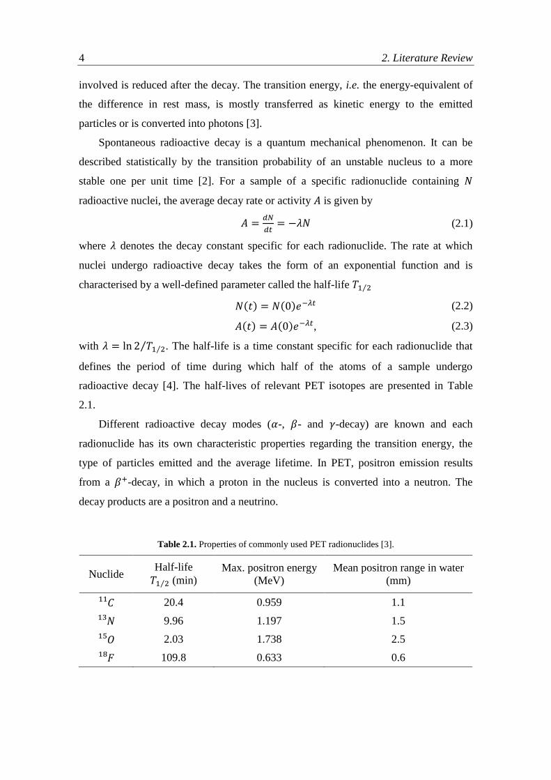
radioactive decay [4]. The half-lives of relevant PET isotopes are presented in Table
2.1.
Different radioactive decay modes (𝛼-, 𝛽- and 𝛾-decay) are known and each
radionuclide has its own characteristic properties regarding the transition energy, the
type of particles emitted and the average lifetime. In PET, positron emission results
from a 𝛽+-decay, in which a proton in the nucleus is converted into a neutron. The
decay products are a positron and a neutrino.
Table 2.1. Properties of commonly used PET radionuclides [3].
Nuclide Half-life
𝑇1 2⁄ (min) Max. positron energy
(MeV)
Mean positron range in water
(mm)
𝐶11 20.4 0.959 1.1
𝑁13 9.96 1.197 1.5
𝑂15 2.03 1.738 2.5
𝐹18 109.8 0.633 0.6

2.1. Basic Principles of Positron Emission Tomography 5
2.1.1.2. Interaction of Positrons with Matter
After emission from the nucleus, the positron interacts with the surrounding matter,
losing kinetic energy. The interaction of positrons with matter depends on their kinetic
energy. Positrons may interact with nuclei or atomic electrons in elastic collisions, with
deflection of the positron and conservation of kinetic energy and linear momentum.
Elastic collisions are not important for charged-particle energy loss and detection [5]. In
contrast, larger fractions of the proton’s kinetic energy are transferred to the shell
electrons of surrounding atoms during inelastic collisions. As a result, the atom is
ionised or excited. Also, inelastic scattering with nuclei may occur, with positron
deflection and loss of its kinetic energy by emitting electromagnetic radiation, the so-
called Bremsstrahlung (i.e. braking radiation). Bremsstrahlung does not play a dominant
role for standard positron emitters applied in PET. When nearly at rest, the positron
combines with an electron, with subsequent annihilation, resulting in two 511 keV
photons (the rest-mass equivalent of each particle) emitted in opposite directions (180°)
to conserve momentum (Figure 2.1).
Figure 2.1. Positron emission and subsequent annihilation resulting in two 511 keV annihilation photons
with opposite directions. Adapted from [6].
Positron-emitting
radionuclide
Positron
Annihilation
511 keV
photon
511 keV
photon
Electron

6 2. Literature Review
2.1.1.3. Interaction of Photons with Matter
Photons are neutral particles with zero rest-mass, which allows them to travel long
distances without interacting with the surrounding medium. Photons coming from the
subject under examination are detected by the interactions with the detector material,
such as the scintillation crystals. In case of the 511 keV annihilation photons, there are
two main mechanisms of interaction with matter relevant for PET: the photoelectric
effect and the Compton scattering. The photoelectric effect describes an interaction
between a photon and a bound atomic electron (from an inner shell), leading to the
ejection of the electron from the atom (Figure 2.2). As a result of the interaction, the
photon is absorbed and its energy is transferred to the electron. The kinetic energy of the
free electron corresponds to the difference between the photon’s energy and the
electron’s binding energy.
Figure 2.2. Photoelectric effect. Adapted from [3].
Compton scattering is the interaction between a photon and a loosely-bound
electron (inelastic collision). The energy of the photon is partly transferred to the
electron, which is ejected from the atom, and the photon undergoes a change in
direction and energy (Figure 2.3).
In both interactions the absorption process creates an energetic electron that is able
to move through the crystal and interact with other atomic electrons, which in the end
leads to the production of scintillation light.
Ejected electron
Incident
photon

2.1. Basic Principles of Positron Emission Tomography 7
Figure 2.3. Compton scattering. Adapted from [3].
In case of lower energy photons (< 100 keV), the dominant interaction is the
photoelectric effect for materials with lower atomic number, e.g. body tissues (𝑍 ≲ 20)
[4]. For energies between 100 keV and ~10 MeV the dominant effect is Compton
scattering, as illustrated in Figure 2.4.
Figure 2.4. Dominating interaction versus photon energy for different atomic numbers [4].
Incident
photon Scattered
photon
θ Scattering angle
Ejected
electron
Photon energy (MeV)
Ato
mic
nu
mb
er,
Z
Compton
scattering
Pair
production Photoelectric
effect
8 2. Literature Review
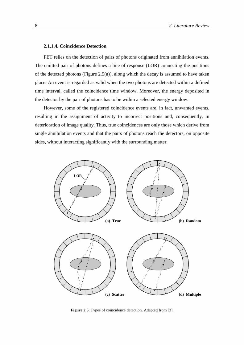
2.1.1.4. Coincidence Detection
PET relies on the detection of pairs of photons originated from annihilation events.
The emitted pair of photons defines a line of response (LOR) connecting the positions
of the detected photons (Figure 2.5(a)), along which the decay is assumed to have taken
place. An event is regarded as valid when the two photons are detected within a defined
time interval, called the coincidence time window. Moreover, the energy deposited in
the detector by the pair of photons has to be within a selected energy window.
However, some of the registered coincidence events are, in fact, unwanted events,
resulting in the assignment of activity to incorrect positions and, consequently, in
deterioration of image quality. Thus, true coincidences are only those which derive from
single annihilation events and that the pairs of photons reach the detectors, on opposite
sides, without interacting significantly with the surrounding matter.
Figure 2.5. Types of coincidence detection. Adapted from [3].
(a) True (b) Random
(c) Scatter (d) Multiple
LOR
2.1. Basic Principles of Positron Emission Tomography 9
A significant number of photons travelling from the annihilation point towards the
detector undergo Compton scattering (Figure 2.5(c)), which is the most probable
interaction of the 511 keV annihilation photons, as mentioned in the previous section.
Also, random coincidences are detected when photons from unrelated annihilation
events occur simultaneously, being counted within the timing window, while their
counterparts are lost (Figure 2.5(b)). These events are initially regarded as valid and are
assigned to an incorrect LOR. These events lead to an overestimation of the tracer
distribution and reduction in image contrast [7]. Finally, multiple coincidences are
similar to random events and occur when more than two photons are detected within the
coincidence time window (Figure 2.5(d)). In these situations, the ambiguity in deciding
which pair of photons arises from the same annihilation event usually leads to the
rejection of the events.
2.1.2. Data Corrections
Methodological approaches to correct for various sources of error are required in
order to achieve qualitative and quantitative PET data. In this context, corrections can
be considered to have their source of error on the interaction of photons with matter,
such as scattering, attenuation and random coincidences, or on the characteristics of the
scanner, namely normalisation and dead time effects. These are some of the most
important corrections required when dealing with PET data and are briefly mentioned
hereafter.
2.1.2.1. Compton scattering
Accurate scatter corrections are an important aspect for quantitative PET imaging.
Scatter results in decreased image contrast and overestimation of tracer distribution,
meaning not only qualitative degradation, but also quantitative inaccuracy.
Since there is a reduction in photon energy after scattering events, energy resolution
has to be as good as possible so that only photons with reasonable image information
are accepted, i.e. only photons exceeding a certain energy threshold are regarded as
valid. However, events with small scattering angles can be accepted with this energy
discrimination.

10 2. Literature Review
Various approaches for estimating and correcting scattered coincidences have been
proposed. Scatter can be estimated analytically or numerically. For instance, Monte
Carlo simulations are capable of providing accurate results, but are not fast enough to be
used in clinical routine. The currently used single scatter simulation (SSS) is a
computationally fast 3D algorithm applied in PET scatter correction. This algorithm
estimates the expected single scatter coincidence rate considering that only one of the
two annihilation photons is scattered. Multiple scatter events are considered less likely
to occur. Further information on this topic can be found in [8, 9].
2.1.2.2. Attenuation
As already mentioned, when travelling through the matter, photons interact, mainly
by Compton scattering, and lose energy. The attenuation process depends on the
transmission length and on the linear attenuation coefficient 𝜇 of the medium, which in
turn depends on the photon energy [10]. Therefore, two annihilation photons may pass
different materials and be attenuated with different probabilities.
Correction factors are needed for each LOR in order to correct images for
attenuation. In conventional PET, the correction factors are usually extracted from
transmission sources. Attenuation can be directly measured with one or multiple
rotating radiation sources (with energies around 511 keV) placed outside the subject.
Alternatively, attenuation correction factors can be extracted from images of the
subject acquired with CT or MRI. In case of PET/CT, the CT data represent
transmission scans that can be scaled to the right energy of 511 keV. However, the MR
images can only be used indirectly, as they represent proton densities, rather than
electron densities. Segmentation of MR images and template-based approaches have
been developed in this context [11, 12].
2.1.2.3. Random Coincidences
The rate of detected random coincidences is related to the rate of single events on
each detector and to the width/length of the timing window. Random coincidences
occur homogeneously across the field of view (FOV), adding a homogeneous
background that becomes more prominent with increasing count rates. Good temporal
resolution is mandatory in order to keep random coincidence rates low.
2.1. Basic Principles of Positron Emission Tomography 11
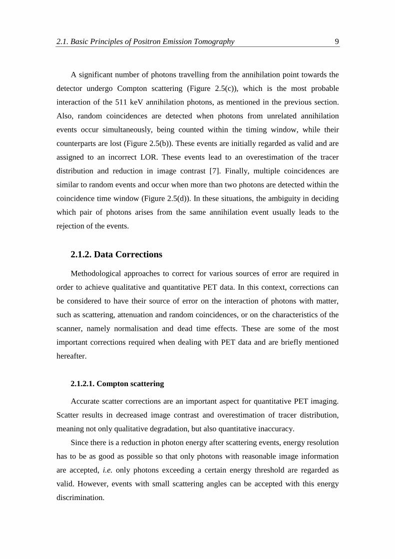
The delayed time window approach is a commonly used method for random counts
correction [2]. This approach includes a normal timing window, during which both true
and random coincidences are detected, and a second timing window (the delayed
window) measuring random coincidences (Figure 2.6). The probability of detecting a
true coincidence in the delayed time window is thus assumed to be null. Since the time
windows’ width is the same, the rate of random events is estimated to be equal in both
windows and the randoms can be subtracted directly from the coincidence data [13].
Figure 2.6. Delayed window approach. The coincidence window represents true and random events and
the delayed window only random events. Adapted from [2].
2.1.2.4. Normalisation
Normalisation is another process of correction required for the reconstruction of
quantitative and artefact-free images. Crystals exhibit varying detection efficiencies,
resulting in LORs with inhomogeneous detection efficiencies among the detector.
Therefore, individual correction factors for each LOR are required. A plane source
measurement is usually performed to acquire the normalisation data. The plane source is
placed at the centre of the FOV, which is rotated to a number of different positions [14].
The data from the different views is then merged into a normalisation file, considering
only the data from LORs perpendicular to the plane source of every view. This
Coincidence
window
Delayed
window
Time difference between detected events
Nu
mb
er o
f ev
ents

12 2. Literature Review
normalisation file contains the different detector and geometric sensitivities of the
scanner [3, 12].
2.1.2.5. Detector Dead Time
The time required by a detector to process an incoming event, during which no
further events can be processed, is known as dead time. This causes an underestimation
of voxel value of the reconstructed image. With increasing activity, the probability of
two or more events occurring within this time period increases.
The dead time effects are significant and additionally can vary within detector
blocks among the scanner. Different correction models have been proposed, such as an
exponential correction model to describe the dead time of a PET scanner on block level
[15, 16]. For the correction of measurement data, parameters for these dead time
correction models can be derived from decay experiments [12, 7].
2.1.3. Data Organisation and Image Reconstruction
PET data can be acquired in either 2D or 3D modes. Regarding the temporal
information data can also be acquired in different modes, such as the standard list-mode
acquisition. With this acquisition mode spatial and temporal information as well as
other characteristics of the photon, e.g. the energy, are recorded for each detected event.
After list-mode acquisition, data is usually stored into sinograms, which can be directly
used for image reconstruction. A sinogram for each transaxial place is acquired in 2D
data. Each LOR is defined by the distance 𝑟 of the LOR from the centre of the FOV and
the angle of orientation 𝜙 the LOR (Figure 2.7). The sinogram is thus a 2D histogram of
the LORs in the (𝑟, 𝜙) Cartesian coordinate system in a given (transaxial) plane. In 3D
acquisitions two more variables are needed for the parametrisation of the LORs: the
angle 𝜃 that defines the angle between the LOR and the transaxial plane and the
coordinate 𝑧 which is the position in the axial direction [17, 3].
There are two basic approaches for the reconstruction of PET images: the analytic
and the iterative reconstruction. Analytic reconstruction algorithms require the prior
correction of the acquired data. They have the advantage of being computationally fast
and straight-forward [2], but have some drawbacks related with the introduction of

2.1. Basic Principles of Positron Emission Tomography 13
blurring in images. The filtered backprojection is the standard analytic reconstruction
method applied in PET [2, 6, 3].
Figure 2.7. Schematic representation of a ring scanner. The sinogram variables 𝒓 and 𝝓 define the
location and orientation of the LOR [3].
Iterative reconstruction is in turn computationally demanding, with longer
computation times than analytic methods, but more accurate and realistic in the
modelling of imaging process and system response [18]. These methods take into
account the statistical properties of the acquired data and noise.
Although there is a variety of iterative reconstruction algorithms, most of them fit a
general model structure (Figure 2.8). The iteration begins with an initial estimate of the
voxel intensity values of the image, which is forward-projected and compared with the
measured data to create a set of projection-space error values. These are then back-
projected to the image space in order to obtain image-space error values that are used to
update the image estimate. This process is repeated with the new image estimate until
some ending criterion is reached [2].
The maximum-likelihood expectation-maximisation (MLEM) algorithm and its
variants (e.g. the ordered-subset expectation-maximisation (OSEM) algorithm) are the
most commonly used iterative reconstruction algorithms in PET [19, 20].
Detector A
Detector B
LOR
𝒓
𝝓
y
x

14 2. Literature Review
Figure 2.8. Generic model structure of iterative reconstruction algorithms. Adapted from [2].
2.2. Basic Principles of Magnetic Resonance Imaging
Magnetic resonance imaging (MRI) is a medical imaging technique that allows the
imaging of anatomical structures with high spatial resolution and soft tissue contrast.
Also the delivery of information on perfusion, diffusion and chemical composition of
tissue, are such characteristics that make MRI one of the most important imaging
modalities in medicine.
For imaging purposes the hydrogen nucleus, containing a single proton, is used due
to its abundance in water and fat. However, MRI is not only capable of providing
imaging of protons (1H), but also other nuclei less abundant in biological tissues such as
sodium (23
Na) and phosphorus (31
P) [21].
When compared to CT imaging, MRI provides better soft tissue contrast and at the
same time avoids the use of ionizing radiation.
Projection
Comparison
Backprojection
Update
Estimated
projections
Measured
projections
Projection
space
error
Image
space
error
Image
estimate
New Old
Image space Projection space

2.2. Basic Principles of Magnetic Resonance Imaging 15
2.2.1. Physical Principles
2.2.1.1. Spin and Nuclear Magnetic Resonance
Atomic nuclei with an odd number of protons and/or neutrons possess spin angular
momentum, which give rise to the quantum mechanical property of nuclear magnetic
resonance (NMR).
Protons possess spin, an intrinsic property of almost all elementary particles.
Besides having angular momentum, the proton has magnetic momentum and behaves
like a small magnet, which means it is influenced by external magnetic fields and
electromagnetic waves. In the presence of an external magnetic field 𝐵0, the spins
magnetic moment �⃗� tend to align in the direction of 𝐵0, assumed as the z-direction or
longitudinal direction. Also, nuclear spins undergo precession (Figure 2.9) at a well-
defined frequency called the Larmor frequency 𝜔. This frequency is related to the
strength of the applied magnetic field by the expression
𝜔 = 𝛾𝐵0 (2.4)
where the gyromagnetic ratio 𝛾 is a known constant that depends on the type of nucleus.
Figure 2.9. External magnetic field (𝑩𝟎) effect on a proton. The proton precesses about the
magnetic field, with its precessional axis parallel to 𝑩𝟎 [22].
Most whole-body human imaging systems use magnetic fields of 1.5 𝑇 and 3 𝑇 in
clinical practice, and 7 𝑇 up to 9.4 𝑇 in clinical and preclinical research [7].
𝑩𝟎
𝒛
𝒚
𝒙
𝝎

16 2. Literature Review
While the spin-system reaches a stable state, a net magnetisation vector �⃗⃗⃗� is set
along the patient axis (z-axis) as a result of the sum of all the individual magnetic
moments. The magnetisation vector has its major contribution in the direction of 𝐵0,
which corresponds to the longitudinal magnetisation 𝑀𝑧.
To obtain an MR signal, a radio frequency (RF) pulse is oriented perpendicular to
𝐵0 and tuned to the resonant frequency (𝜔) of the spins. The RF pulse is produced by a
transmission coil placed close to the imaging volume. This manipulation of the
magnetisation in the transverse (xy) plane excites the spins out of equilibrium and forces
them to rotate in phase, increasing the transverse magnetisation 𝑀𝑥𝑦. The angle by
which the net magnetisation is rotated away from the main magnetic field direction (z-
axis) is known as the flip angle 𝛼 [23].
2.2.1.2. Relaxation
After excitation, the return of the net magnetisation vector �⃗⃗⃗� back to its thermal
equilibrium state is observed. The term relaxation describes this phenomenon and is
well defined by the relaxation time constants 𝑇1 and 𝑇2. The spin-lattice interaction
refers to the 𝑇1 relaxation (or longitudinal relaxation) and characterises the return of �⃗⃗⃗�
along the z-direction, that is, the 𝑀𝑧 recovery after application of the RF pulse (Figure
2.10). For a 90° excitation (𝑀𝑧(0) = 0) this exponential behaviour is described by
𝑀𝑧 = 𝑀0(1 − 𝑒−𝑡 𝑇1⁄ ), (2.5)
where 𝑀0 corresponds to the net magnetisation strength (i.e. the equilibrium
magnetisation). The behaviour of the transverse component of the magnetisation vector
is characterised by the spin-spin time constant which is referred to as 𝑇2 or transverse
relaxation (Figure 2.10). This process results in the decay of 𝑀𝑥𝑦 and thus in MR signal
loss. Following a 90° excitation (𝑀𝑥𝑦(0) = 𝑀0), this process is given by
𝑀𝑥𝑦 = 𝑀0𝑒−𝑡 𝑇2⁄ . (2.6)
𝑇1 and 𝑇2 relaxation time constants, along with the proton density 𝑝, are important
MR parameters which values vary with the tissue under investigation. In practice, static
field inhomogeneities and 𝑇2 decay are observed, resulting in a reduced relaxation time
constant 𝑇2∗. The loss of MR signal due to 𝑇2
∗ effects is known as free induction decay
(FID).

2.2. Basic Principles of Magnetic Resonance Imaging 17
Figure 2.10. Proton relaxation processes: spin-lattice or longitudinal relaxation (left) and spin-spin or
transverse relaxation (right).
2.2.1.3. Imaging Principles
When excited, the spins behave like oscillators inducing signals at the Larmor
frequency. The total signal (FID signal) generated by all oscillators of the excited area is
recorded in a single time waveform, containing no spatial information. So in order to
achieve spatial information, linear gradient fields �⃗� are applied in addition to 𝐵0. These
gradient fields can be switched independently in all directions and are therefore
denominated as 𝐺𝑥, 𝐺𝑦 and 𝐺𝑧. To note that the combined magnetic field (for instance,
𝐵0 + 𝑥𝐺𝑥 if a gradient 𝐺𝑥 is applied in the x-direction) still points in the z-direction,
only field strength varies. The superposition of gradient fields forces the spins at
different locations to precess at different frequencies, thus allowing a selective
excitation. Slice selection is consequently achieved as the gradient field is applied
within a specific range of frequencies (bandwidth).
Phase- and frequency-encoded data is stored in the Fourier space, or k-space,
according to the spatial location, and is analysed by the Fourier transform. Image
reconstruction can be performed by applying an inverse Fourier transform of the k-
space.
2.2.2. MRI Sequences
MRI pulse sequences consist of programmed sets of changing RF pulses and
magnetic gradients, which are grouped together into an MRI protocol. There are two
basic classes of sequences: the spin-echo (SE) pulse sequence and the gradient-echo
𝑴𝒙𝒚(𝒕) 𝑴𝒛(𝒕)
0 𝑻𝟏 Time
𝟎. 𝟔𝟑 𝑴𝒛
0 𝑻𝟐 Time
𝟎. 𝟑𝟕 𝑴𝒙𝒚
Spin-lattice relaxation Spin-spin relaxation
18 2. Literature Review
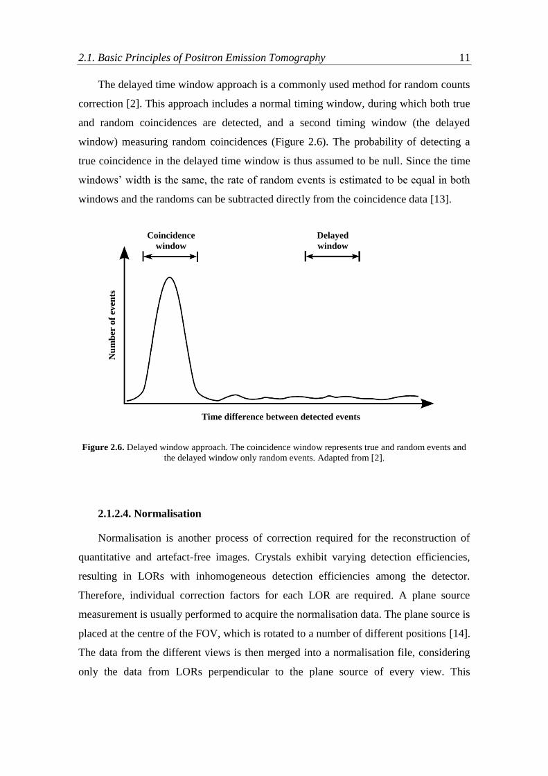
(GE) pulse sequence. The SE sequence is the most commonly used in MRI. This pulse
sequence can be adjusted to give 𝑇1-weighted, proton density and 𝑇2-weighted images.
The term spin-echo refers to the refocusing of precessing spin magnetisation by a 180°
pulse at the Larmor frequency (Figure 2.11(a)). The sequence begins with the
simultaneous application of a slice selection gradient 𝐺𝑧 and a 90° RF excitation pulse.
After this, phase- and frequency-encoding gradients, 𝐺𝑦 and 𝐺𝑥 respectively, are
applied. As it is known, the observed MR signal decays with time due to spin-spin
relaxation and magnetic field inhomogeneities (𝑇2∗). The loss of transverse
magnetisation can be partly recovered by a 180° refocusing pulse. This pulse is applied
at 𝑡 = 𝑇𝐸 2⁄ and the so called spin-echo is created at 𝑡 = 𝑇𝐸 (Figure 2.11(b)), where
the parameter 𝑇𝐸 refers to the echo time. Because 𝑇2 dephasing is only partly
reversible, the maximum of the spin-echo is lower than the maximum signal intensity at
𝑡 = 0. The time between two 90° RF excitations is the repetition time (TR).
Figure 2.11. Diagram of a spin-echo pulse sequence (a) and corresponding time signal (b) [24].
90º 180º
𝑮𝒛
𝑮𝒚
𝑮𝒙
RF
(a)
(b)
90º 180º
𝑻𝟐∗ 𝑻𝟐
∗
𝑻𝟐
TE
RF
Signal
𝑻𝑬
𝟐
Readout

2.2. Basic Principles of Magnetic Resonance Imaging 19
Figure 2.12. Diagram of a gradient-echo pulse sequence [24].
The major drawback of SE sequences is the long imaging times, particularly in
proton density and 𝑇2-weighted imaging protocols (as TR is extended to minimize the
influence of 𝑇1 relaxation). To overcome this problem GE sequences are used. As
compared to SE sequences, they mainly differ in two respects: the application of flip
angles that are usually smaller than 90° and the absence of the 180° refocusing pulse
(i.e. there is no spin-echo). The reduced flip angle leads to a smaller transverse
magnetisation, resulting in faster longitudinal magnetisation and, therefore, shorter TR.
The rephasing is done by gradient reversal, which implies that the loss of signal results
from 𝑇2∗ effects. This sequence is thus more sensitive to magnetic field artefacts than SE
sequences (Figure 2.12).
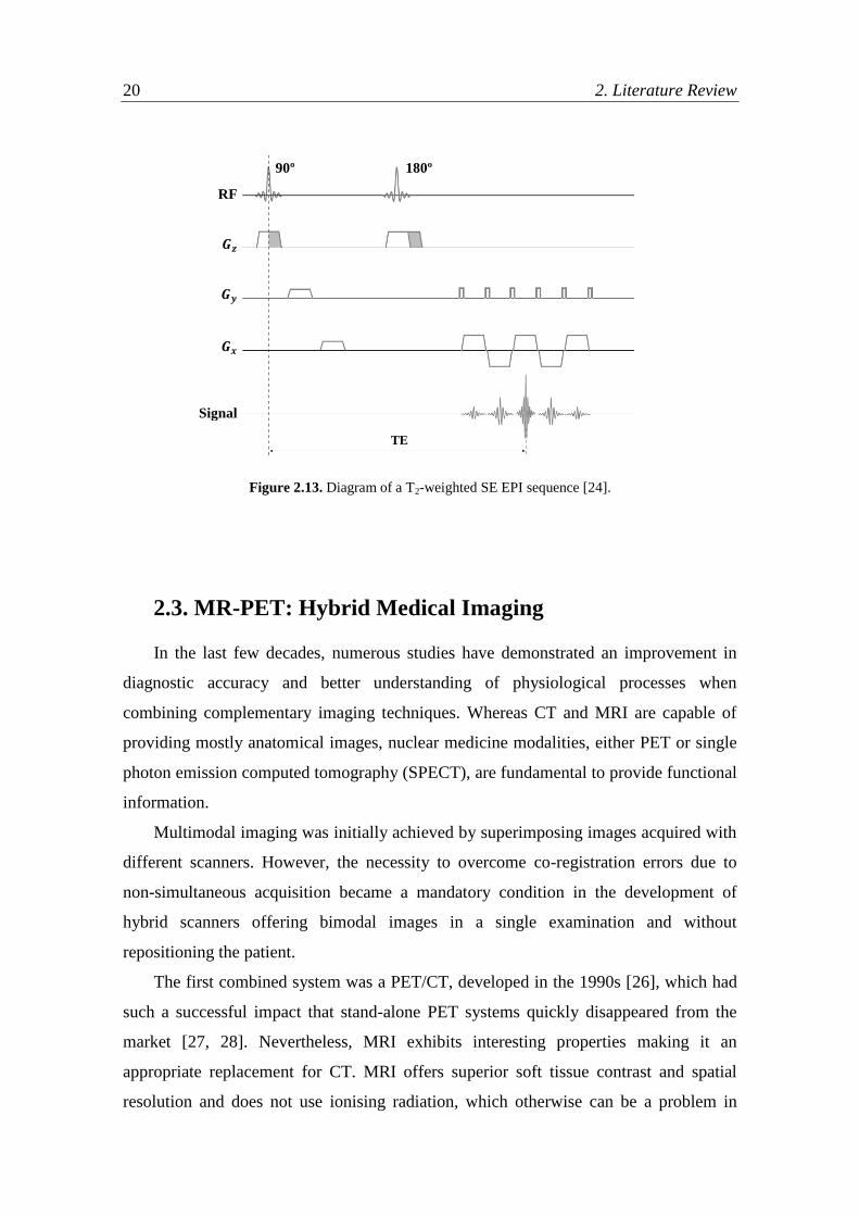
An approach to overcome longer MR acquisitions is the development of very fast
imaging sequences, such as echo-planar imaging (EPI). EPI is performed using a rapid
gradient switching to acquire multiple echoes generated and sampled within the same
excitation (Figure 2.13) [25]. A typical matrix size of EPI images is 128 × 128 and
images can be acquired in 20 – 100 ms, allowing a very high temporal resolution. This
is of great importance since it allows less motion artefacts and also the ability to image
rapid physiologic and kinetic processes of the human body [21, 24]. However, EPI is
more sensitive to susceptibility effects and magnetic field inhomogeneities and the
obtained signal is more 𝑇2∗-weighted. Concerning the equipment, it requires high
performance gradient coils. The EPI sequence is used, for instance, in functional
(fMRI), diffusion and perfusion imaging.
𝑮𝒛
𝑮𝒚
𝑮𝒙
RF
𝜶
Readout
20 2. Literature Review
Figure 2.13. Diagram of a T2-weighted SE EPI sequence [24].
2.3. MR-PET: Hybrid Medical Imaging
In the last few decades, numerous studies have demonstrated an improvement in
diagnostic accuracy and better understanding of physiological processes when
combining complementary imaging techniques. Whereas CT and MRI are capable of
providing mostly anatomical images, nuclear medicine modalities, either PET or single
photon emission computed tomography (SPECT), are fundamental to provide functional
information.
Multimodal imaging was initially achieved by superimposing images acquired with
different scanners. However, the necessity to overcome co-registration errors due to
non-simultaneous acquisition became a mandatory condition in the development of
hybrid scanners offering bimodal images in a single examination and without
repositioning the patient.
The first combined system was a PET/CT, developed in the 1990s [26], which had
such a successful impact that stand-alone PET systems quickly disappeared from the
market [27, 28]. Nevertheless, MRI exhibits interesting properties making it an
appropriate replacement for CT. MRI offers superior soft tissue contrast and spatial
resolution and does not use ionising radiation, which otherwise can be a problem in
90º 180º
𝑮𝒛
𝑮𝒚
𝑮𝒙
RF
Signal
TE

2.3. MR-PET: Hybrid Medical Imaging 21
paediatrics and when repetitive or follow-up studies are required. Furthermore, MRI
also possesses different applications in the domain of functional imaging, such as
diffusion weighted imaging (DWI) and MR spectroscopy which, moreover, do not rely
on the injection of contrast agents [28]. Thus, although PET offers the possibility of
studying a wider spectrum of metabolic functions with higher sensitivity, the
advantages of whole-body MR-PET are not limited to the complementary imaging of
anatomy by MRI and function by PET, but include simultaneous combined functional
imaging of each modality.
2.3.1. Advantages and Challenges of Combing PET and MRI
Besides the MRI advantages already mentioned over CT, there are some other
benefits from the use of hybrid MR-PET scanners. Even with PET/CT scans, MRI scans
are often required for further information, meaning that simultaneous MR-PET
measurements increase patient comfort and reduce scan times.
Another advantage of hybrid MR-PET systems is the fact that the acquisition times
of MRI and PET do not differ as much as those of CT and PET. This reduced time
difference offers the opportunity to really perform simultaneous imaging which might
result in qualitatively new ways for investigating functional processes [28]. Also
improvements in co-registration of simultaneous MR-PET systems can be derived from
the MR images. With the fast acquisition of MR images using the EPI sequence (in the
range of seconds), motion parameters can be extracted, allowing thus motion corrected
PET and MRI data without external motion tracking [7, 29].
When combining two imaging modalities in a single system there are some
technological challenges of possible mutual interferences that have to be overcome. The
first obstacle is the incompatibility of the photomultiplier tubes (PMTs) and magnetic
fields. Conventional PET systems use PMTs to detect the scintillation light. However,
since they are very sensitive to magnetic fields, PMTs cannot be operated inside an MR
scanner. As a result, some approaches have been studied in order to overcome this
problem, such as the use of optical fibres to guide the scintillation light from the crystals
to PMTs placed outside the MR system, or the use of avalanche photodiodes (APDs)
and, more recently, silicon photomultipliers (SiPMs) to replace conventional PMTs.
Another challenge is the fast switching gradients and the RF fields influence in PET
22 2. Literature Review
electronics, which need proper shielding. Also, PET electronics may in turn cause
magnetic field inhomogeneities, which have to be compensated by appropriate
shimming, and signal-to-noise ratio (SNR) degradation. An additional difficulty in MR-
PET scanners, and an active topic of research nowadays, is the attenuation correction,
which is a prerequisite for accurate quantitative PET. Unlike the attenuation maps
provided by CT, there is no relation between the MR image intensity and the attenuating
properties of the tissue (valid for 511 keV photon radiation) [30]. Hence, the attenuation
data have to be derived from MR images [31].
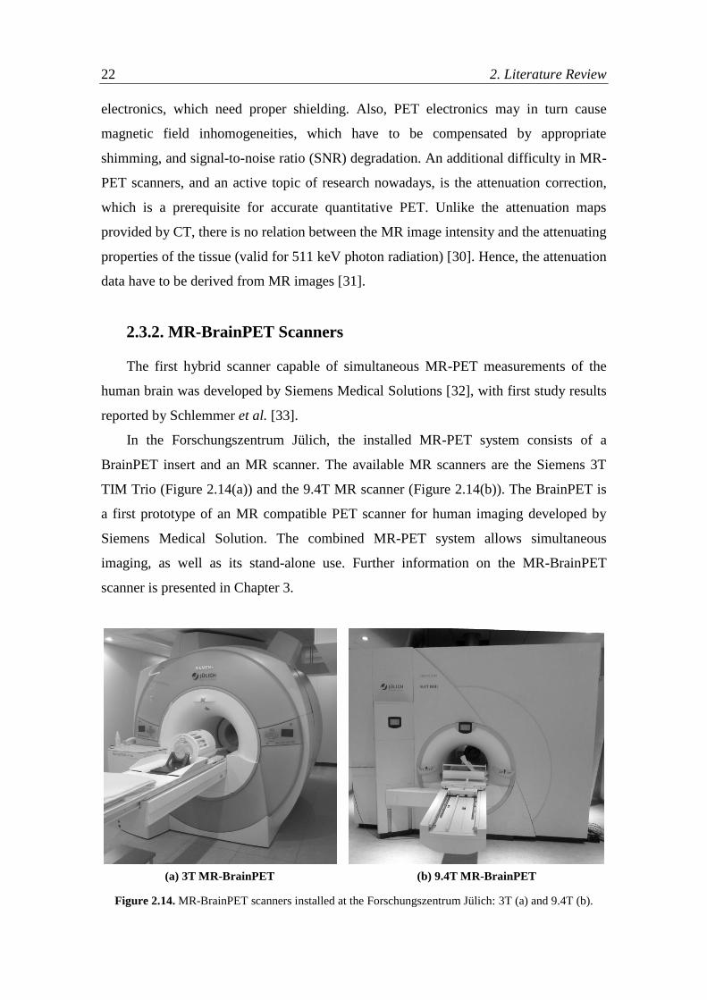
2.3.2. MR-BrainPET Scanners
The first hybrid scanner capable of simultaneous MR-PET measurements of the
human brain was developed by Siemens Medical Solutions [32], with first study results
reported by Schlemmer et al. [33].
In the Forschungszentrum Jülich, the installed MR-PET system consists of a
BrainPET insert and an MR scanner. The available MR scanners are the Siemens 3T
TIM Trio (Figure 2.14(a)) and the 9.4T MR scanner (Figure 2.14(b)). The BrainPET is
a first prototype of an MR compatible PET scanner for human imaging developed by
Siemens Medical Solution. The combined MR-PET system allows simultaneous
imaging, as well as its stand-alone use. Further information on the MR-BrainPET
scanner is presented in Chapter 3.
Figure 2.14. MR-BrainPET scanners installed at the Forschungszentrum Jülich: 3T (a) and 9.4T (b).
(a) 3T MR-BrainPET (b) 9.4T MR-BrainPET
2.4. Dynamic Imaging 23
2.4. Dynamic Imaging
2.4.1. Dynamic PET
Dynamic, or four-dimensional (4D), PET is able to produce parametric images of
physiological processes, which often have greater clinical utility than static 3D
images [34]. In order to assess these parametric or quantitative biological images,
suitable data corrections and reconstruction algorithms (briefly mentioned in previous
PET section), as well as accurate biological models are required [18].
Mathematical models (i.e. kinetic models) relating the dynamics of the tracer and
its biological states to the resultant PET image are used in order to determine the signal
of interest. Compartmental models are often used to modulate the tracer kinetics. Each
possible tracer’s state is considered as a compartment (where tracers are uniformly
distributed in space), independent of others and with characteristic volume,
concentration and chemical reactions.
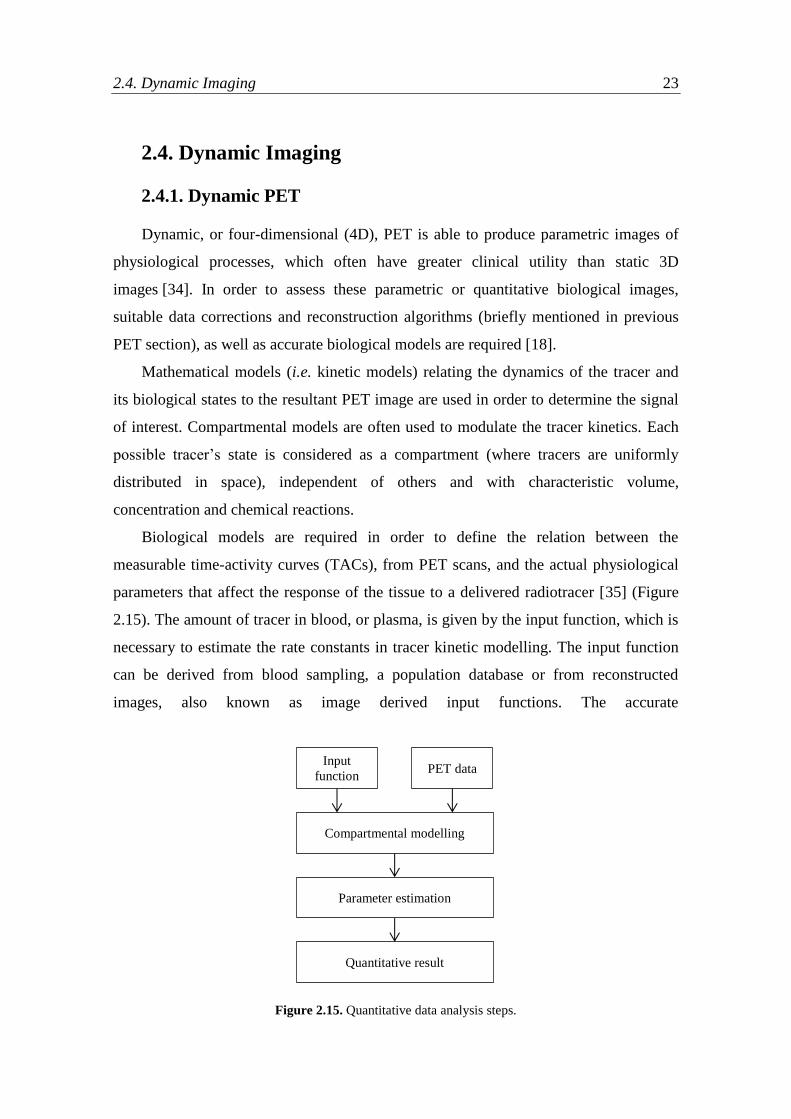
Biological models are required in order to define the relation between the
measurable time-activity curves (TACs), from PET scans, and the actual physiological
parameters that affect the response of the tissue to a delivered radiotracer [35] (Figure
2.15). The amount of tracer in blood, or plasma, is given by the input function, which is
necessary to estimate the rate constants in tracer kinetic modelling. The input function
can be derived from blood sampling, a population database or from reconstructed
images, also known as image derived input functions. The accurate
Figure 2.15. Quantitative data analysis steps.
Input
function PET data
Compartmental modelling
Parameter estimation
Quantitative result

24 2. Literature Review
measurement of input function is mandatory to successful quantitative imaging [35].
The kinetic analysis can be processed on a voxel-by-voxel basis, producing parametric
images, or on a region of interest (ROI) basis, grouping voxels from homogeneous
structures [18]. While a regional analysis allows to process data with better statistics
and reduced computing times, as only the average radioactivity of the voxels within a
ROI are analysed (instead of thousands of voxels), a voxel-by-voxel analysis is far more
complex since the TAC of a single voxel is highly influenced by the noise.
Nevertheless, this latter type of analysis might provide better knowledge on the local
physiology.
2.4.1.1. Measuring the Amino acid Kinetics
Radiolabelled amino acids have proven to be useful in the diagnostic of brain
tumours [36]. The 18
F-labelled amino acid O-(2-[18
F]fluoroethyl)-L-tyrosine (FET, half-
life: 109.8 min) is a PET tracer that shows a strongly increased uptake in cerebral
tumours, whereas the uptake in inflammatory cells and the cortex is relatively low,
yielding good tumour-to-background contrast [37]. Moreover, the FET uptake enables
the discrimination between different tumour grading (low- and high-grade) in both
untreated and recurrent gliomas [36, 38].
FET is not incorporated into proteins. Its high uptake in tumour cells is due to the
increased transport via the L-system amino acid transporters1 [39]. Particularly, FET is
more selectively transported through LAT2 than through LAT1 (Figure 2.16). As a
consequence, this tracer overcomes the limitations of [18
F]-FDG by showing higher
specificity and, therefore, higher tumour-to-background contrast (Figure 2.17).
Figure 2.16. Molecular structure of the FET tracer (a) and its selectivity in the L-system amino acid
transporters LAT1 and LAT2 (b). Adapted from [38].
1 L-type amino acid transporters (LATs) are the major transport system for large neutral amino acid,
of which subtypes 1 (LAT1) and 2 (LAT2) have been related to the cellular uptake of FET in tumour cells
[40, 41].
(a) (b)

2.4. Dynamic Imaging 25
For all these reasons, FET-PET has gained increasing interest in clinical imaging
and, consequently, much information on kinetic analysis have been proposed, but still
remains a matter of discussion [36, 42].
Figure 2.17. [18
F]-FDG and [18
F]-FET PET contrast images, showing higher tumour-to-background
contrast with FET. Adapted from [43].
2.4.2. Dynamic MRI
Dynamic susceptibility contrast (DSC) MRI is the most commonly used method for
estimation of perfusion parameters, such as cerebral blood flow (CBF) [44]. Also
known as bolus-tracking MRI, DSC-MRI requires the injection of a paramagnetic
contrast agent and the fast acquisition of the MR signal loss during its passage through
the tissue. The bolus of contrast agent induces a transient signal loss on 𝑇2- and
𝑇2∗-weighted images [45].
DSC-MRI kinetics can be expressed by the convolution expression [46, 44]:
𝐶(𝑡) = 𝐶𝐵𝐹 ⋅ 𝐴𝐼𝐹(𝑡) ⨂ 𝑅(𝑡) = 𝐶𝐵𝐹 ⋅ ∫ 𝐴𝐼𝐹(𝜏)𝑅(𝑡 − 𝜏)𝑑𝜏𝑡
0
(2.7)
where 𝐶(𝑡) is the time-dependent concentration of the contrast agent, 𝐴𝐼𝐹(𝑡) is the so-
called arterial input function (more information can be found in [44]) and 𝑅(𝑡) is the
impulse response function or residue function, which describes the fraction of contrast
agent remaining in the tissue after an instantaneous input bolus.
Although it requires the use of an exogenous contrast agent, DSC-MRI is a very
powerful perfusion imaging method due to the wealth of information that can be
extracted from the acquired data. Also, its fast acquisition times and use of standard
MRI sequences (e.g. EPI), as well as good contrast-to-noise ratio, are some of the
reasons why DSC-MRI is such a popular and currently the most used brain perfusion
imaging method.

26 2. Literature Review
2.4.2.1. MRI Contrast Agents
Image contrast in MRI results from differences in signal intensity, which is
determined by the properties of the different tissues (intrinsic factors, such as
differences in the 𝑇1 and/or 𝑇2 relaxation times) and the properties of the used pulse
sequence (extrinsic factors, like the actual sequence or the chosen TR and TE values).
Despite the inherent high contrast of MR images, these signal differences can be
further enhanced by the administration of contrast agents (Figure 2.18), which can
additionally provide dynamic (pharmacokinetic) information. MRI contrast agents alter
the intrinsic contrast properties of biological tissues either by changing the proton
density of the tissue or by changing the local magnetic field or the resonance properties
of the tissue and, therefore, its 𝑇1 and/or 𝑇2 values [23].
Figure 2.18. T1-weighted magnetisation-prepared rapid acquisition with gradient echo (MP-RAGE)
without contrast medium (left) and T1-weighted MP-RAGE with contrast medium (right) [47].
Most of clinically available MR contrast media consist of paramagnetic substances,
typically gadolinium-based contrast agents [44]. These contrast media substances are
mostly toxic metal ions, particularly the gadolinium-based ones, which belongs to the
lanthanide series of rare-earth elements. Gadolinium is toxic, in part, by blocking
calcium channels, so it must be chelated with an appropriate ligand to allow clinical
use [48].
2.4.2.2. Modelling DSC-MRI time-concentration curves
When calculating perfusion parameters it is usual to model time-concentration
curves (TCCs) by an analytic function. Given the nature of the contrast bolus, the AIFs
and also the tissue concentration curves display a peaked shape, with a baseline period
(before the arrival of the bolus), followed by a peak (the first passage of the contrast

2.4. Dynamic Imaging 27
agent) and a slower decrease (not returning to baseline values) with a second smaller
and wider peak coming afterwards, which is often referred to as the recirculation.
Various functions have been proposed to model the AIFs and, therefore, tissue
TCCs. The gamma-variate (GV) function is one of the most commonly used models
[44, 49]:
𝑦(𝑡) = 𝐴(𝑡 − 𝑡0)𝛼𝑒−(𝑡−𝑡0)/𝛽 (2.8)
valid for 𝑡 > 𝑡0, where A is a scaling factor, 𝛼 and 𝛽 determine the shape of the curve
and 𝑡0 the time at which the bolus arrives at a given region, also referred to as the bolus
arrival time (BAT). This function has been often used to describe tracer dilution curves
[50, 51, 52]. Thompson et al. [50] showed that gamma variates could be fitted to tracer
dilution curves with very good agreement.
As previously mentioned, the GV function is generally applied to fit indicator
dilution curves, which supported the decision of choosing this method to do the fitting
of the analysed data in the current project (which will be discussed hereafter). So,
although this subject comes following this modelling section of dynamic MRI, the GV
function has similar applications in nuclear medicine [50, 53, 54, 55].


29
3. Materials and Methods
3.1. The MR-BrainPET Scanner
The clinical data analysed in this work was acquired with the Siemens 3T MR-
BrainPET system. As mentioned in Section 2.3, the BrainPET insert was designed to be
MR-compatible. For simultaneous MR and PET measurements, the BrainPET is placed
inside the bore of the MR scanner (Figure 3.1), with a 36 cm opening for the MR head
coil – an adapted head coil with low attenuation for the 511 keV photons [56]. Thus,
this configuration minimises attenuation, as well as scatter, as the annihilation photons
only need to go through the head coil until reaching the PET detectors.
Figure 3.1. The 3T MR-BrainPET installed at the Forschungszentrum Jülich (since 2008). This hybrid
scanner consists of a MAGNETOM Trio MRI and the BrainPET insert (placed between the magnet and
the MR coils) [27].

30 3. Materials and Methods
3.1.1. BrainPET Component
The BrainPET component consists of 32 copper-shielded detector cassettes, each
containing 6 detector blocks with a 12 × 12 LSO2 crystal matrix (with a crystal size of
2.5 × 2.5 × 20 mm3 each), placed in a ring. The crystal matrix is read out by a 3 × 3
array of APDs. The signals from the detector cassettes are transmitted via shielded
cables of 10 m length and connected to a data acquisition system. The scanner has an
axial FOV of about 20 cm and a transaxial FOV of 36 cm (the inner diameter). Further
information on the scanner configuration can be found in [28, 12].
3.1.2. Data Acquisition Modes
The data acquisition systems of the two parts of the 3T MR-BrainPET are
independent of each other. In particular, the BrainPET scanner has two acquisition
modes: the single and the coincidence modes. While the single mode is used for scanner
performance evaluation and setup purposes, the coincidence acquisition mode is the
standard mode used for imaging purposes [12].
Coincidence data can be acquired in list-mode or LOR-mode. Each entry of the list-
mode data represents a detected event in chronological order. Time markers with high
temporal resolution (at intervals of 200 μs [27]) are inserted for posterior framing. List-
mode files allow flexible post-processing, which means they can be histogrammed into
sinograms after the measurement and divided into predefined time frames. This framing
allows the evaluation of the dynamic radiotracer distribution as a function of time. All
PET data analysed in this work was recorded in list-mode.
3.2. Measurements
For this study, simultaneously acquired PET and MRI data on 12 brain tumour
patients were used. All scans were carried out on the hybrid 3T MR-BrainPET. Several
datasets were analysed, all of which referring to patients with histologically confirmed
cerebral glioma and meningioma, some were untreated and others had undergone
previous tumour resection, radiation and/or chemotherapy (or a combination thereof).
Some relevant protocol details are briefly mentioned hereafter.
2 Lutetium oxyorthosilicate.

3. Materials and Methods 31
3.2.1. PET Protocols
PET was performed using [18
F]-FET. For this purpose, FET at a dose of 3 MBq/kg
of body weight was injected at the start of the PET acquisition. PET data was acquired
for 60 min after injection in list-mode and framed into 23 time frames with variable
frame length (8 × 5 𝑠, 2 × 10 𝑠, 2 × 15 𝑠, 1 × 30 𝑠, 1 × 60 𝑠, 1 × 120 𝑠, 5 × 300 𝑠
and 3 × 600 𝑠). Image reconstruction was performed using the clinical standard 3D
ordinary Poisson OSEM (OP-OSEM) scheme with 4 subsets and 32 iterations. The
reconstructed images have 256 × 256 × 153 isotropic voxels of (1.25 mm)3. Once the
image is reconstructed, the resulting voxel intensities were converted into activity
concentrations (e.g. Bq/mL) instead of counts using a calibration factor. Moreover, the
reconstructed images were post-filtered with a 2 mm Gaussian filter.
3.2.2. MRI Protocols
All MRI sequences were acquired simultaneous to the PET measurement. During
the dynamic acquisition, a varied number of sequences can be performed, for instance,
for structural and functional imaging (e.g. MP-RAGE3 and EPI, respectively). Standard
MRI protocols begin with a localizer sequence (2D gradient echo) recorded to check the
positioning of the head, followed by a T1-weighted MP-RAGE, which is an anatomical
sequence. Other sequences composing the MR protocol are not mentioned, as they are
not relevant for this study. In this context, DSC-MRI was acquired based on EPI
sequence with an echo time of 32 ms and a repetition time of 1500 ms. The matrix size
was 128 × 128 voxels and 20 slices with a voxel size of 1.8 × 1.8 × 5.0 mm3
were
acquired. Contrast agent4 was injected during the EPI measurement at a dose of
0.1 mmol/kg of body weight.
3 Magnetisation-prepared rapid acquisition with gradient echo (MP-RAGE) sequence.
4 Dotarem
® (gadoterate meglumine) – an MRI gadolinium-based contrast agent indicated for
intravenous use in e.g. brain studies to help detecting and visualising areas with disruption of the blood
brain barrier and/or abnormal vascularity.

32 3. Materials and Methods
3.3. Data Analysis
Patient motion introduces blurring in images, which is even more evident in scans
with long periods of acquisition, such as the one hour dynamic [18
F]-FET PET scans.
Furthermore, in dynamic analysis performed based on voxel intensity or ROIs, motion
correction is important to avoid voxel/ROI mispositioning and therefore incorrect
dynamic information. In this context, motion correction was performed using PMOD’s
image registration and fusion tool (PFUS). Images were motion corrected relatively to a
reference image, which corresponded to an average image calculated from a range of
the first frames (excluding the initial noisy frames) with negligible patient motion.
Motion was visually assessed having an anatomical structure, e.g. nose, to determine the
reference frames and the ones to be corrected.
Image registration was performed with PMOD’s fusion tool as well (cross-modality
rigid matching), having the anatomical MP-RAGE images as reference. Both PET and
MRI images were motion corrected and co-registered following the same steps.
For the dynamic analysis, data was post-processed using MATLAB. After loading
the data from both modalities, the dynamic images were filtered using a 2 mm Gaussian
filter. Various width (sigma) values were tested in order to obtain better results. In
general, the SNR of dynamic EPI images is relatively low, as opposed to the FET ones,
which are usually very noisy. As a result, special attention was focused on the filtering
of FET data to facilitate the fitting and extraction of information from the TACs.
The DSC-MRI data was converted into TCCs, 𝑐(𝑡), by using
𝑐(𝑡) = −1
𝑇𝐸ln (
𝑆(𝑡)
𝑆0) (3.1)
where 𝑆(𝑡) corresponds to the MRI signal and 𝑆0 is the prebolus baseline signal
intensity, which was considered to be the first five frames of each time series [57].
The analysis was carried out on a voxel-by-voxel basis. Features from both
modalities were extracted in order to produce parametric images of peak, time to peak
(TTP), area under the curve (AUC) and wash-in (Figure 3.2). TTP was considered as
the time from the start of the injection until maximum contrast concentration is reached;
and peak was obtained from the maximum calculated for each curve. AUC was obtained
calculating the integral of each curve, whilst wash-in was estimated from the maximum
slope of the curve.

3. Materials and Methods 33
Figure 3.2. Graph illustrating a contrast time curve plotted from a normal brain tissue. Parametric images
are obtained from the extracted features, such as peak, TTP, AUC, and wash-in, represented in this curve.
Adapted from [58].
The correct fitting of the data is important, as the extraction of some features can be
affected by the function that is adjusted to the contrast-time curves. Consequently, the
fitting applied to the curves was performed using the GV function (Section 2.4.2.2.). To
solve this function by running a least-squares estimation algorithm, initial coefficient
values are required, i.e. initial guess values of the dependent variables 𝐴, 𝛼, 𝛽 and 𝑡0. It
is important to note that poor starting values can lead to a solution with large residual
error, as verified in the resulting simulations. While running the first fits, the initial
guess values were manually adjusted to the curves. The fitted curves were visually
checked to guarantee reasonable fits. Although the adjustment was only applied to a
single exemplary curve for each dataset (and then run for the remaining curves), the
process was neither efficient, nor prompt when analysing several datasets. Therefore,
the estimation of the initial guesses of the four variables was simplified by extracting
information from each curve. In this way the maximum of the curve and the time to
peak were used to aid the determination of the initial guess of 𝐴 and 𝑡0, respectively. 𝐴
was set to the value of the maximum (𝑦𝑚𝑎𝑥) multiplied by a scaling factor to adjust to
the curve (i.e. a scalar manually adjusted for the curve). The parameter 𝑡0 was set to the
value of the onset of the bolus, which was determined by searching from the time point
Peak
TTP
Area under the curve
Wash-in
Time
Co
ntr
ast
ag
ent
con
cen
trati
on

34 3. Materials and Methods
of the maximum (𝑡𝑚𝑎𝑥) back to the origin looking for two successive values lying under
a threshold of 10% of the maximum, as suggested by Benner et al. [59].
At last, the simplified formulation of the GV function derived by Madsen [52] was
applied, enabling one to obtain the four initial guess values required to run the least-
squares algorithm, mentioned hereafter as the automated method. The only estimates
required are 𝑡0 (the onset of the bolus, which can be simplified by assuming 𝑡0 = 0),
𝑡𝑚𝑎𝑥 and 𝑦𝑚𝑎𝑥, all of which can be estimated with the derived expressions by Madsen
[52]. Further information on the mentioned simplified formulation of the GV function
can be found in the Appendix.
While doing the GV curve fitting of the data, a parameter variation analysis was
done in order to better understand the changes in the shape and fit of the curves, i.e. a
variation in each GV parameter was analysed (keeping the remaining constant).
Additionally, an AIF fitting analysis testing the manual and automated fitting methods
was done, with the AIFs extracted with the Stroketool software.

35
4. Results and Discussion
As already mentioned, the broad outline of this project was to generate parametric
images from dynamic MR-PET data and compare the extracted information from both
modalities. Therefore, this chapter is organised as a sequence of results through the
analysis course. Firstly, some data filtering results are shown. The analyses regarding
the GV fitting model are presented afterwards. FET-PET and MRI curves and the
resulting fitted ones are exemplified. As a consequence of these last results, a parameter
variation analysis (of the GV function) was performed in order to better understand the
behaviour of the fitted curves when varying the GVs. Furthermore, an AIF fitting
analysis is presented, in which different fitting methods were tested. At last, some
analysed datasets and their corresponding extracted parametric images are presented.
4.1. Data Filtering
As already mentioned, FET data is highly influenced by the noise, requiring
appropriate data correction methods and reconstruction algorithms and also suitable
filtering methods. In this context, a Gaussian filter using different width values (Figure
4.1) was tested. The resulting images led to the selection of the 2 mm as the
No filter
2 mm
3 mm
Figure 4.1. Images extracted from the FET data: an example of unfiltered image (left) and the
corresponding filtered ones with 2 mm (middle) and 3 mm width (right).
50 100 150
50
100
150
200
250
50 100 150
50
100
150
200
250
50 100 150 200 250
50
100
150
200
250
50 100 150
50
100
150
200
250
50 100 150
50
100
150
200
250
AUC 90,110
50 100 150 200 250
50
100
150
200
250
0
0.5
1
1.5
2
2.5
x 107
0
5
10
15
x 106
0
2
4
6
8
10
12
x 106
0
5
10
15
x 106
0
0.5
1
1.5
2
2.5
x 107
0
5
10
15
x 106
50 100 150
50
100
150
200
250
50 100 150
50
100
150
200
250
50 100 150 200 250
50
100
150
200
250
50 100 150
50
100
150
200
250
50 100 150
50
100
150
200
250
AUC 90,110
50 100 150 200 250
50
100
150
200
250
0
1
2
3
4
x 107
0
0.5
1
1.5
2
2.5
3
x 107
0
1
2
3
4
x 107
0
1
2
3
4
5
x 107
0
1
2
3
4
5
x 107
0
0.5
1
1.5
2
2.5
3
3.5
x 107
50 100 150
50
100
150
200
250
50 100 150
50
100
150
200
250
50 100 150 200 250
50
100
150
200
250
50 100 150
50
100
150
200
250
50 100 150
50
100
150
200
250
AUC 90,110
50 100 150 200 250
50
100
150
200
2500
2
4
6
8
x 107
0
2
4
6
8
x 107
0
2
4
6
8
x 107
0
2
4
6
8
x 107
0
2
4
6
8
x 107
0
2
4
6
8
x 107
50 100 150
50
100
150
200
250
50 100 150
50
100
150
200
250
50 100 150 200 250
50
100
150
200
250
50 100 150
50
100
150
200
250
50 100 150
50
100
150
200
250
AUC 90,110
50 100 150 200 250
50
100
150
200
250
0
1
2
3
4
x 107
0
0.5
1
1.5
2
2.5
3
x 107
0
1
2
3
4
x 107
0
1
2
3
4
5
x 107
0
1
2
3
4
5
x 107
0
0.5
1
1.5
2
2.5
3
3.5
x 107

36 4. Results and Discussion
filter width to apply to the reconstructed data. Also, the Gaussian filter implemented by
the PMOD software was tested, although all images were processed using MATLAB, it
was useful in the motion correction step (to aid in the detection of movement). Once
again, the selected filter, with which better results were achieved, was the 2 mm one, as
showed in Figure 4.2.
A different approach in the filtering process may be beneficial and help to obtain
less noisy TACs that are more easily described and fitted by a known mathematical
function. Thus enabling one to produce more accurate parametric images, as the adopted
methods might have somehow limited the results.
Figure 4.2. An FET-PET image filtered using the PMOD software (2 mm filter).
4.2. Gamma-variate Fitting
For the voxel-by-voxel analysis, the TCCs obtained are exemplified in Figure 4.3
and Figure 4.4. In these figures, the resulting GV fitted curves are also shown. For the
EPI curves (Figure 4.3), a good fit of the observed data was achieved. However, for the
TACs extracted from FET data (Figure 4.4), it was not possible to apply a fit to all
image voxels. The main reason for these findings is probably due to the noisy nature of
the FET curves. While in the MR data, even though there are some voxels in which it is
not possible to properly fit the data, a GV function can be applied to the majority of the
TCCs.

4. Results and Discussion 37
Figure 4.3. EPI contrast-time curves from a single voxel analysis and the corresponding adjusted
GV function.
The fitted GV parameters were estimated having the automated method suggested
by Madsen [52] as starting point. It was not possible to establish a relation between the
estimated GV parameters that better fitted the curves, i.e. the parameters (𝐴, 𝛼, 𝛽 and
𝑡0) obtained for one curve did not resemble the values of other curves even within the
same subject. For instance, changes in 𝛼 and 𝛽 were found to affect both the location
and magnitude of the function’s maximum, and also the rise and fall times of the
function, as illustrated in Figure 4.5. In fact, both variations (in 𝛼 and 𝛽) were found to
be very similar when merging the plots in Figure 4.5 together.
0 10 20 30 40 50 60 70 80-5
0
5
10
15
20
25
30
35
40
45
Time [s]
Concentr
ation o
f contr
ast agent [a
.u.]
Contrast-time curve
Fitted curve
0 10 20 30 40 50 60 70 80-5
0
5
10
15
20
25
Time [s]
Concentr
ation o
f contr
ast agent [a
.u.]
Contrast-time curve
Fitted curve

38 4. Results and Discussion
Figure 4.4. FET-PET time-activity curves from a single voxel analysis and the corresponding adjusted
GV function. The levels of noise observed in the FET-derived curves hampered the fitting process, and in
some cases have made it unsuccessful.
In the same line of analysis, changes in 𝐴 and 𝑡0, as described in literature, only
produce effects in the magnitude and onset of the peak (Figure 4.6), respectively,
without changing its shape.
Another finding while doing this parameter variation analysis was that different sets
of GV parameter values can produce similar curves. Figure 4.7 illustrates an AIF
(dashed line) and two different fitted curves, one of them (red line) representing the
adjusted curve with initial guess values: 𝛼 and 𝛽 fixed at 3 and 1.5 s, respectively,
which are reference values used in AIF simulations (representative of typical data in
adults) as reported in [46, 45]; while 𝐴 and 𝑡0 were manually adjusted for each
0 20 40 60 80 100 120 140 160 1800
10
20
30
40
50
60
70
80
Time [s]
FE
T c
oncentr
ation [kB
q/c
c]
Time-activity curve
Fitted curve
0 20 40 60 80 100 120 140 160 1800
1
2
3
4
5
6
7
8
9
Time [s]
FE
T c
oncentr
ation [kB
q/c
c]
Time-activity curve
Fitted curve

4. Results and Discussion 39
Figure 4.5. Plots of the GV function showing the differences in the location and magnitude of the curves
when varying 𝜶 (plots on the left) and 𝜷 (plots on the right) and keeping the remaining parameters
constant. Also the rise and fall times are affected with these changes.
curve. The parameters for the other fitted curve (black line) were set with the initial
values given by the automated method (i.e. following the simplified formulation of the
GV function). Clearly the fitted curves differ in shape, but there are some similarities
between them and are both considered acceptable fits of the AIF, yet the values of the
estimated GVs are different.
Figure 4.6. Plots of the GV function showing the differences in the amplitude and onset of the curves
when varying 𝑨 (plots on the left) and 𝒕𝟎 (plots on the right), respectively, and keeping the remaining
parameters constant. As expected, no changes in the shape of the curves were observed.
0 10 20 30 40 50 60 70 800
20
40
60
80
100
120
A=1.105E-4
A=2.105E-4
A=3.105E-4 (mean)
A=4.105E-4
A=5.105E-4
0 10 20 30 40 50 60 70 800
50
100
150
200
250
300
0 10 20 30 40 50 60 70 800
50
100
150
200
250
300
0 10 20 30 40 50 60 70 800
10
20
30
40
50
60
70
0 10 20 30 40 50 60 70 800
20
40
60
80
100
120
A=1.105E-4
A=2.105E-4
A=3.105E-4 (mean)
A=4.105E-4
A=5.105E-4
0 10 20 30 40 50 60 70 800
50
100
150
200
250
300
0 10 20 30 40 50 60 70 800
50
100
150
200
250
300
0 10 20 30 40 50 60 70 800
10
20
30
40
50
60
70
0 10 20 30 40 50 60 70 800
20
40
60
80
100
120
0 10 20 30 40 50 60 70 800
50
100
150
200
250
300
B=8.4249
B=8.7249
B=9.0249 (mean)
B=9.3249
B=9.6249
0 10 20 30 40 50 60 70 800
50
100
150
200
250
300
C=0.9751
C=1.0751
C=1.1751 (mean)
C=1.2751
C=1.3751
0 10 20 30 40 50 60 70 800
10
20
30
40
50
60
70
0 10 20 30 40 50 60 70 800
20
40
60
80
100
120
0 10 20 30 40 50 60 70 800
50
100
150
200
250
300
B=8.4249
B=8.7249
B=9.0249 (mean)
B=9.3249
B=9.6249
0 10 20 30 40 50 60 70 800
50
100
150
200
250
300
C=0.9751
C=1.0751
C=1.1751 (mean)
C=1.2751
C=1.3751
0 10 20 30 40 50 60 70 800
10
20
30
40
50
60
70
y(t
)
y(t
)
t [s] t [s]
0 10 20 30 40 50 60 70 800
20
40
60
80
100
120
A=1.105E-4
A=2.105E-4
A=3.105E-4 (mean)
A=4.105E-4
A=5.105E-4
0 10 20 30 40 50 60 70 800
50
100
150
200
250
300
B=8.4249
B=8.7249
B=9.0249 (mean)
B=9.3249
B=9.6249
0 10 20 30 40 50 60 70 800
50
100
150
200
250
300
C=0.9751
C=1.0751
C=1.1751 (mean)
C=1.2751
C=1.3751
0 10 20 30 40 50 60 70 800
10
20
30
40
50
60
70
BAT=10.3084
BAT=12.3084
BAT=14.3084 (mean)
BAT=16.3084
BAT=18.3084
t0=10.3084
t0=12.3084
t0=14.3084
t0=16.3084
t0=18.3084
0 10 20 30 40 50 60 70 800
20
40
60
80
100
120
A=1.105E-4
A=2.105E-4
A=3.105E-4 (mean)
A=4.105E-4
A=5.105E-4
0 10 20 30 40 50 60 70 800
50
100
150
200
250
300
B=8.4249
B=8.7249
B=9.0249 (mean)
B=9.3249
B=9.6249
0 10 20 30 40 50 60 70 800
50
100
150
200
250
300
C=0.9751
C=1.0751
C=1.1751 (mean)
C=1.2751
C=1.3751
0 10 20 30 40 50 60 70 800
10
20
30
40
50
60
70
BAT=10.3084
BAT=12.3084
BAT=14.3084 (mean)
BAT=16.3084
BAT=18.3084
A=1.105E-4
A=2.105E-4
A=3.105E-4
A=4.105E-4
A=5.105E-4
0 10 20 30 40 50 60 70 800
20
40
60
80
100
120
A=1.105E-4
A=2.105E-4
A=3.105E-4 (mean)
A=4.105E-4
A=5.105E-4
0 10 20 30 40 50 60 70 800
50
100
150
200
250
300
B=8.4249
B=8.7249
B=9.0249 (mean)
B=9.3249
B=9.6249
0 10 20 30 40 50 60 70 800
50
100
150
200
250
300
C=0.9751
C=1.0751
C=1.1751 (mean)
C=1.2751
C=1.3751
0 10 20 30 40 50 60 70 800
10
20
30
40
50
60
70
BAT=10.3084
BAT=12.3084
BAT=14.3084 (mean)
BAT=16.3084
BAT=18.3084
y(t
)
y(t
)
t [s] t [s]
=8.4249
=8.7249
=9.0249
=9.3249
=9.6249
0 10 20 30 40 50 60 70 800
20
40
60
80
100
120
A=1.105E-4
A=2.105E-4
A=3.105E-4 (mean)
A=4.105E-4
A=5.105E-4
0 10 20 30 40 50 60 70 800
50
100
150
200
250
300
B=8.4249
B=8.7249
B=9.0249 (mean)
B=9.3249
B=9.6249
0 10 20 30 40 50 60 70 800
50
100
150
200
250
300
C=0.9751
C=1.0751
C=1.1751 (mean)
C=1.2751
C=1.3751
0 10 20 30 40 50 60 70 800
10
20
30
40
50
60
70
BAT=10.3084
BAT=12.3084
BAT=14.3084 (mean)
BAT=16.3084
BAT=18.3084
=0.9751
=1.0751
=1.1751
=1.2751
=1.3751

40 4. Results and Discussion
Figure 4.7. Plots of an AIF (dashed line) and its fitted curves obtained from the automated (black line)
and manual methods (red line). Better results were verified with the automated fitting model.
4.2.1. AIF Fitting Analysis
This parameter variation analysis resulted from an AIF fitting analysis, in which a
set of AIFs extracted with the Stroketool software from various patient data was
analysed and both manual and automated fitting methods tested. Illustrative plots are
showed in Figure 4.7. As expected, more accurate fits were obtained using the latter
method, i.e. lower mean squared error (MSE) values were registered. The parameter
values of the manual fitting, particularly the obtained 𝛼 and 𝛽 mean values, 2.5±0.6 and
2.9±0.5 respectively, differed from the literature ones previously mentioned (𝛼 = 3 and
𝛽 = 1.5). When analysing Table 4.1 with the GV parameters of the two fitting methods,
Table 4.1. AIF fitting analysis. Mean and standard deviation values of the estimated GV parameters
obtained with the manual and automated fitting methods, for a set of 10 AIFs.
Manual fitting Automated fitting
GV
parameters �̅� 𝜎 �̅� 𝜎
𝐴 10,5 11,8 0,0003 0,0006
𝛼 2,5 0,6 9,0 3,2
𝛽 2,9 0,5 1,2 0,2
𝑡0 17,0 1,4 14,3 1,0
0 10 20 30 40 50 60 70 800
10
20
30
40
50
60
time [s]
C(t
)
AIF (stroketool)
Auto fitting
Manual fitting

4. Results and Discussion 41
it was not possible to establish a relation between the results either from one method or
the other. Particularly when analysing the automated fitting, where the values of 𝐴 and
𝛼 presented high standard deviation values.
4.3. Parametric Images
Results from two of the analysed datasets are presented in Figure 4.8. This figure
shows the MR images from the MP-RAGE and EPI sequences (Figure 4.8a and b from
each dataset (i and ii), respectively), and the corresponding extracted parametric
Figure 4.8. Two analysed datasets (i and ii). MRI images: MP-RAGE (post contrast) (a), EPI (b), and the
corresponding extracted parametric images: peak (c) and AUC (d). FET-PET image (summed image of
20-40 min p.i.) (e) and the corresponding extracted parametric images of peak (f) and AUC (g).
(a)
(b) (c) (d)
(e) (f) (g)
ii.
Peak AUC
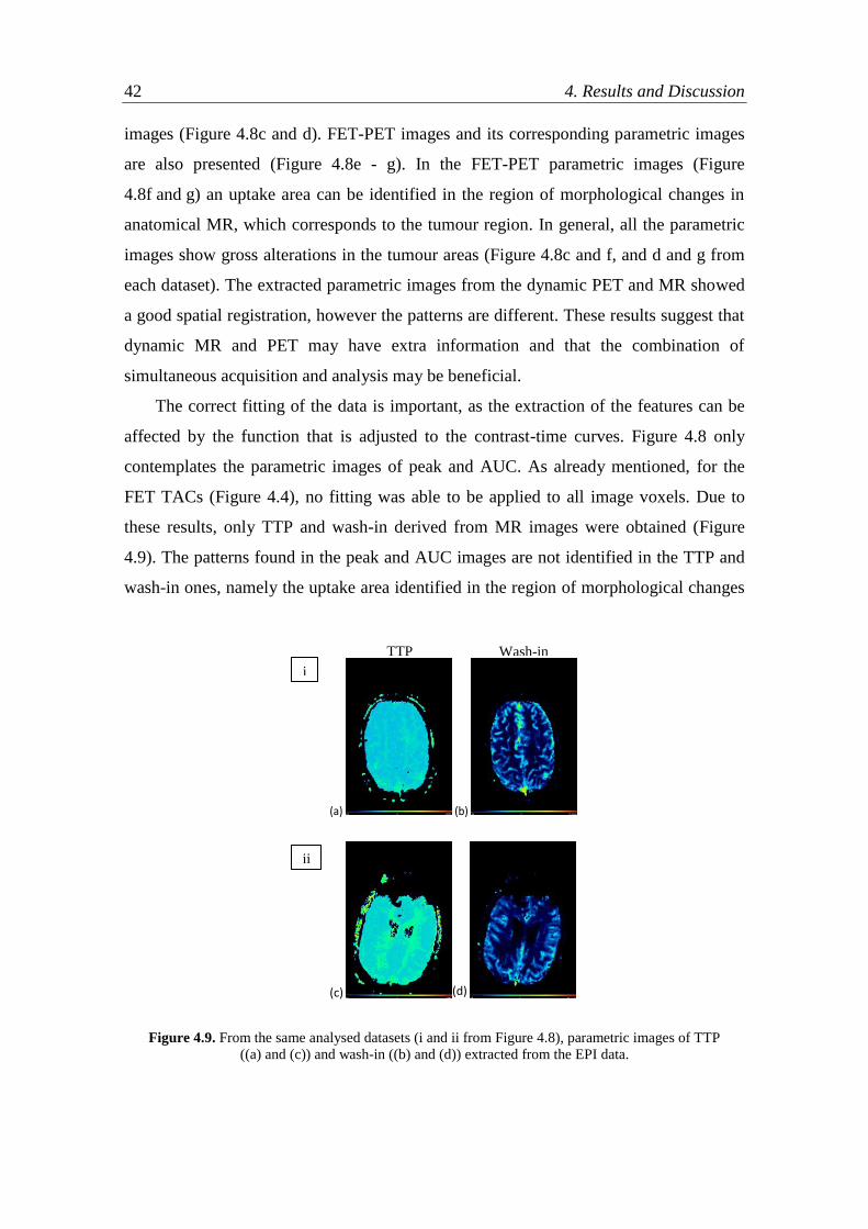
42 4. Results and Discussion
images (Figure 4.8c and d). FET-PET images and its corresponding parametric images
are also presented (Figure 4.8e - g). In the FET-PET parametric images (Figure
4.8f and g) an uptake area can be identified in the region of morphological changes in
anatomical MR, which corresponds to the tumour region. In general, all the parametric
images show gross alterations in the tumour areas (Figure 4.8c and f, and d and g from
each dataset). The extracted parametric images from the dynamic PET and MR showed
a good spatial registration, however the patterns are different. These results suggest that
dynamic MR and PET may have extra information and that the combination of
simultaneous acquisition and analysis may be beneficial.
The correct fitting of the data is important, as the extraction of the features can be
affected by the function that is adjusted to the contrast-time curves. Figure 4.8 only
contemplates the parametric images of peak and AUC. As already mentioned, for the
FET TACs (Figure 4.4), no fitting was able to be applied to all image voxels. Due to
these results, only TTP and wash-in derived from MR images were obtained (Figure
4.9). The patterns found in the peak and AUC images are not identified in the TTP and
wash-in ones, namely the uptake area identified in the region of morphological changes
Figure 4.9. From the same analysed datasets (i and ii from Figure 4.8), parametric images of TTP
((a) and (c)) and wash-in ((b) and (d)) extracted from the EPI data.
(a) (b)
i
.
ii
.
(d) (c)
TTP Wash-in
(c) (d)

4. Results and Discussion 43
in anatomical MR, which might indicate that different data analysis approaches are
required in order to obtain all parametric images (especially TTP images from FET data,
which are particularly interesting and useful in clinical routine).


45
5. General Discussion and Conclusions
The limitations regarding the high noise level of PET data have confirmed one of
this technique’s drawbacks. Even with the data smoothing and all the pre-processing
corrections, PET images noisy nature plays a major role on the analysis and extraction
of parametric images. As a consequence for the analysis exposed in this work, the
purpose of obtaining parametric images from dynamic MR-PET data and the
combination of information from both modalities has been limited for this reason. So,
on the one hand there is this issue which has revealed to be a limitation in achieving all
project goals. On the other hand, the choice of the fitting model to apply to the data
might not have been the most appropriate one.
One thing is certain, and was the reason that supported its choice, the GV function
remains the most commonly used model for hemodynamic studies. However, it presents
several drawbacks which still remain a matter of controversy. Madsen [52] reported that
changes in the 𝛼 and 𝛽 parameters affect not only the location and magnitude of the
peak but also its rise and fall times, leading to uncertainty in the fitting optimisation
process. In fact, this has revealed to be a challenge, mostly while adjusting the initial
gamma-variates for the manual fitting of the TACs, since the slightest change in one of
these parameters would produce modifications in the curves shape. Benner et al. [59]
suggested that the GV fitting is only reliable when time resolution, maximal signal drop
and SNR are kept within reasonable limits and when the initial guess values set for the
least-squares estimation algorithm are ensured to be also reliable, otherwise leading to
unsatisfying results. Furthermore, Li et al. [60] reported that the parameter 𝐴 is
nonlinear and thus needs to be taken into account during the fitting process in order to
obtain unbiased results, as already stated by Thompson et al. [50].
Some other more complex models have been proposed [61, 62, 63]. For instance,
Enmi et al. [63] developed an alternative technique for reconstructing AIFs from TCCs
46 5. General Discussion and Conclusions
of multiple brain regions (as opposed to the usual AIFs obtained from TCCs of a
cerebral artery), by using a multi-exponential function.
Other approaches might have been beneficial, such as a regional analysis, instead of
a voxel-by-voxel analysis, considering only the average concentration curves within a
certain neighbourhood (i.e. within homogeneous structures). This analysis would allow
to process data with better statistics, as well as reduced computing times. Or even an
analysis considering only the area of morphological changes in anatomical MR (i.e. the
tumour region). However, the achievement of parametric images revealing detailed
information on every voxel would not be possible with this approach.
Also, an alternative may pass by testing the GV function and other fitting models
for different curves, adding different levels of noise, and varying the model parameters
so that better knowledge on the curves behaviour is achieved. By quantifying the noise
level and testing which model better fits the data, this approach might be useful when
next applying the model to the FET data.
Overall, the underlying purpose of developing an image analysis tool that can be
used to generate parametric images from different features extracted from dynamic MR-
PET data was partially achieved. The combination and subsequent comparison between
the extracted information from both modalities were not possible, due to the lack of
results from the dynamic PET data. Nevertheless, some parametric images were
obtained and may be useful to provide extra information in tumour assessment.

47
Bibliography
[1] G. Hevesy. The Absorption and Translocation of Lead by Plants, Biochem.
J., vol. 17, pp. 439–445, 1923.
[2] M. N. Wernick and J. N. Aarsvold. Emission Tomography: The
Fundamentals of PET and SPECT. Elsevier Academic Press, 2004.
[3] D. L. Bailey, D. W. Townsend, P. E. Valk, and M. N. Maisey. Positron
Emission Tomography: Basic Sciences. Springer, 2005.
[4] S. R. Cherry, J. Sorenson, and M. E. Phelps. Physics in Nuclear Medicine,
4th ed. Elsevier Inc., 2012.
[5] N. Tsoulfanidis. Measurement and Detection of Radiation, 2nd ed. Taylor &
Francis, 1995.
[6] M. E. Phelps. PET: Physics, Instrumentation, and Scanners. Springer, 2006.
[7] C. Weirich. Quantitative PET Imaging with Hybrid MR-PET Scanners, PhD
thesis. RWTH Aachen University, 2014.
[8] C. Watson, D. Newport, and M. Casey. A single scatter simulation
technique for scatter correction in 3D PET, Three-Dimensional Image
Reconstr. Radiat. Nucl. Med., pp. 255–268, 1996.
[9] C. C. Watson. New, faster, image-based scatter correction for 3D PET,
IEEE Trans. Nucl. Sci., vol. 47, no. 4, pp. 1587–1594, 2000.
[10] J. Carney, D. Townsend, V. Rappoport, and B. Bendriem. Method for
transforming CT images for attenuation correction in PET/CT imaging,
Med. Phys., vol. 33, no. 4, pp. 976–983, 2006.
[11] E. Rota Kops and H. Herzog. Template based attenuation correction for
PET in MR-PET scanners, 2008 IEEE Nucl. Sci. Symp. Conf. Rec., pp.
3786–3789, 2008.
[12] M. Gaens. Analysis, Characterisation and Setup of a Block Detector Used
in a 3TMR-BrainPET System, diploma thesis. Technische Universitat
Dortmund, 2010.

48 Bibliography
[13] D. Brasse, P. E. Kinahan, C. Lartizien, C. Comtat, M. Casey, and C. Michel.
Correction methods for random coincidences in fully 3D whole-body PET:
impact on data and image quality, J. Nucl. Med., vol. 46, no. 5, pp. 859–67,
2005.
[14] T. R. Oakes, V. Sossi, and T. J. Ruth. Normalization for 3D PET with a
low-scatter planar source and measured geometric factors, Phys. Med. Biol.,
vol. 43, no. 4, pp. 961–972, 1998.
[15] S. Yamamoto, M. Amano, S. Miura, H. Iida, and I. Kanno. Deadtime
correction method using random coincidence for PET, J. Nucl. Med., vol.
27, no. 12, pp. 1925–1928, 1986.
[16] M. E. Daube-Witherspoon and R. E. Carson. Unified deadtime correction
model for PET, IEEE Trans. Med. Imaging, vol. 10, no. 3, pp. 267–275,
1991.
[17] F. H. Fahey. Data acquisition in PET imaging, J. Nucl. Med. Technol., vol.
30, no. 2, pp. 39–49, 2002.
[18] H. Zaidi. Quantitative Analysis in Nuclear Medicine Imaging. Springer,
2006.
[19] L. A. Shepp and Y. Vardi. Maximum Likelihood Reconstruction for
Emission Tomography, IEEE Trans. Med. Imaging, vol. 1, no. 2, pp. 113–
122, 1982.
[20] H. M. Hudson and R. S. Larkin. Accelerated image reconstruction using
ordered subsets of projection data, IEEE Trans. Med. Imaging, vol. 13, no.
4, pp. 601–609, 1994.
[21] D. G. Nishimura. Principles of Magnetic Resonance Imaging. Department
of Electrical Engineering, Stanford University, 1996.
[22] M. A. Brown and R. C. Semelka. MRI: Basic principles and applications,
3rd ed. John Wiley & Sons, Inc., 2003.
[23] D. Weishaupt, V. D. Köchli, and B. Marincek. How Does MRI Work? An
Introduction to the Physics and Function of Magnetic Resonance Imaging,
2nd ed. Springer. Berlin, Heidelberg, 2006.
[24] P. Suetens. Fundamentals of Medical Imaging, 2nd ed. Cambridge
University Press, 2009.
[25] R. L. DeLaPaz. Echo-planar imaging, Radiographics, vol. 14, no. 5, pp.
1045 –1058, 1994.
[26] T. Beyer, D. Townsend, and T. Brun. A combined PET/CT scanner for
clinical oncology, J. Nucl. Med., vol. 41, pp. 1369–1379, 2000.
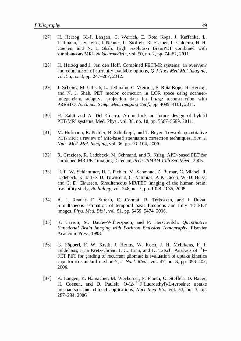
Bibliography 49
[27] H. Herzog, K.-J. Langen, C. Weirich, E. Rota Kops, J. Kaffanke, L.
Tellmann, J. Scheins, I. Neuner, G. Stoffels, K. Fischer, L. Caldeira, H. H.
Coenen, and N. J. Shah. High resolution BrainPET combined with
simultaneous MRI, Nuklearmedizin, vol. 50, no. 2, pp. 74–82, 2011.
[28] H. Herzog and J. van den Hoff. Combined PET/MR systems: an overview
and comparison of currently available options, Q J Nucl Med Mol Imaging,
vol. 56, no. 3, pp. 247–267, 2012.
[29] J. Scheins, M. Ullisch, L. Tellmann, C. Weirich, E. Rota Kops, H. Herzog,
and N. J. Shah. PET motion correction in LOR space using scanner-
independent, adaptive projection data for image reconstruction with
PRESTO, Nucl. Sci. Symp. Med. Imaging Conf., pp. 4099–4101, 2011.
[30] H. Zaidi and A. Del Guerra. An outlook on future design of hybrid
PET/MRI systems, Med. Phys., vol. 38, no. 10, pp. 5667–5689, 2011.
[31] M. Hofmann, B. Pichler, B. Scholkopf, and T. Beyer. Towards quantitative
PET/MRI: a review of MR-based attenuation correction techniques, Eur. J.
Nucl. Med. Mol. Imaging, vol. 36, pp. 93–104, 2009.
[32] R. Grazioso, R. Ladebeck, M. Schmand, and R. Krieg. APD-based PET for
combined MR-PET imaging Detector, Proc. ISMRM 13th Sci. Meet., 2005.
[33] H.-P. W. Schlemmer, B. J. Pichler, M. Schmand, Z. Burbar, C. Michel, R.
Ladebeck, K. Jattke, D. Townsend, C. Nahmias, P. K. Jacob, W.-D. Heiss,
and C. D. Claussen. Simultaneous MR/PET imaging of the human brain:
feasibility study, Radiology, vol. 248, no. 3, pp. 1028–1035, 2008.
[34] A. J. Reader, F. Sureau, C. Comtat, R. Trébossen, and I. Buvat.
Simultaneous estimation of temporal basis functions and fully 4D PET
images, Phys. Med. Biol., vol. 51, pp. 5455–5474, 2006.
[35] R. Carson, M. Daube-Witherspoon, and P. Herscovitch. Quantitative
Functional Brain Imaging with Positron Emission Tomography, Elsevier
Academic Press, 1998.
[36] G. Pöpperl, F. W. Kreth, J. Herms, W. Koch, J. H. Mehrkens, F. J.
Gildehaus, H. a Kretzschmar, J. C. Tonn, and K. Tatsch. Analysis of 18
F-
FET PET for grading of recurrent gliomas: is evaluation of uptake kinetics
superior to standard methods?, J. Nucl. Med., vol. 47, no. 3, pp. 393–403,
2006.
[37] K. Langen, K. Hamacher, M. Weckesser, F. Floeth, G. Stoffels, D. Bauer,
H. Coenen, and D. Pauleit. O-(2-[18
F]fluoroethyl)-L-tyrosine: uptake
mechanisms and clinical applications, Nucl Med Bio, vol. 33, no. 3, pp.
287–294, 2006.

50 Bibliography
[38] C. Kratochwil, S. E. Combs, K. Leotta, A. Afshar-Oromieh, S. Rieken, J.
Debus, U. Haberkorn, and F. L. Giesel. Intra-individual comparison of 18
F-
FET and 18
F-DOPA in PET imaging of recurrent brain tumors, Neuro.
Oncol., vol. 16, no. 3, pp. 434–440, 2014.
[39] D. Pauleit, A. Zimmermann, G. Stoffels, D. Bauer, M. O. Flu, K. Hamacher,
H. H. Coenen, and K. Langen. PET Compared with 18
F-FDG PET and CT
in Patients with Head and Neck Cancer, J. Nucl. Med., vol. 47, no. 2, pp.
256–261, 2006.
[40] P. Heiss, S. Mayer, M. Herz, H. J. Wester, M. Schwaiger, and R.
Senekowitsch-Schmidtke. Investigation of transport mechanism and uptake
kinetics of O-(2-[18
F]fluoroethyl)-L-tyrosine in vitro and in vivo, J. Nucl.
Med., vol. 40, no. 8, pp. 1367–1373, 1999.
[41] M. K. Nedergaard, K. Kristoffersen, S. R. Michaelsen, J. Madsen, H. S.
Poulsen, M. T. Stockhausen, U. Lassen, and A. Kjaer. The use of
longitudinal 18
F-FET MicroPET imaging to evaluate response to irinotecan
in orthotopic human glioblastoma multiforme xenografts, PLoS One, vol. 9,
no. 6, p. e100009, 2014.
[42] N. L. Jansen, B. Suchorska, V. Wenter, S. Eigenbrod, C. Schmid-Tannwald,
A. Zwergal, M. Niyazi, M. Drexler, P. Bartenstein, O. Schnell, J.-C. Tonn,
N. Thon, F.-W. Kreth, and C. la Fougere. Dynamic 18
F-FET PET in Newly
Diagnosed Astrocytic Low-Grade Glioma Identifies High-Risk Patients, J.
Nucl. Med., vol. 55, no. 2, pp. 198–203, 2014.
[43] N. Silva. On the Use of Image Derived Input Function for Quantitative PET
Imaging with a Simultaneous Measuring MR-BrainPET, MSc thesis.
Universidade de Lisboa, Faculdade de Ciências, 2012.
[44] F. Calamante. Arterial input function in perfusion MRI: A comprehensive
review, Prog. Nucl. Magn. Reson. Spectrosc., vol. 74, pp. 1–32, 2013.
[45] F. Calamante, D. G. Gadian, and A. Connelly. Delay and dispersion effects
in dynamic susceptibility contrast MRI: simulations using singular value
decomposition, Magn. Reson. Med., vol. 44, no. 3, pp. 466–473, 2000.
[46] L. Østergaard, R. Weisskoff, D. Chesler, C. Gyldensted, and B. Rosen. High
resolution measurement of cerebral blood flow using intravascular tracer
bolus passages. Part I: Mathematical approach and statistical analysis, Magn
Reson Med, vol. 36, no. 5, pp. 715–725, 1996.
[47] H. Herzog, K.-J. Langen, J. Kaffanke, C. Weirich, I. Neuner, G. Stoffels, E.
R. Kops, J. Scheins, L. Tellmann, and N. J. Shah. MR-PET opens new
horizons in neuroimaging, Future Neurol., vol. 5, no. 6, pp. 807–815, 2010.
[48] T. Ishiguchi and S. Takahashi. Safety of gadoterate meglumine (Gd-DOTA)
as a contrast agent for magnetic resonance imaging: results of a post-

Bibliography 51
marketing surveillance study in Japan, Drugs R. D., vol. 10, no. 3, pp. 133–
45, 2010.
[49] N. D. Forkert, J. Fiehler, T. Ries, T. Illies, D. Möller, H. Handels, and D.
Säring. Reference-based linear curve fitting for bolus arrival time estimation
in 4D MRA and MR perfusion-weighted image sequences, Magn. Reson.
Med., vol. 65, no. 1, pp. 289–294, 2011.
[50] H. K. Thompson, C. F. Starmer, R. E. Whalen, and H. D. McIntosh.
Indicator Transit Time Considered as a Gamma Variate, Circ. Res., vol. 14,
no. 6, pp. 502–515, Jun. 1964.
[51] R. Davenport. The Derivation of the Gamma-Variate Relationship for
Tracer Dilution Curves, J. Nucl. Med., vol. 24, pp. 945–948, 1983.
[52] M. T. Madsen. A simplified formulation of the gamma variate function,
Phys. Med. Biol., vol. 37, no. 7, pp. 1597–1600, 1992.
[53] H. Kelbaek, O. J. Hartling, K. Skagen, O. Munck, O. Henriksen, and J.
Godtfredsen. First-pass radionuclide determination of cardiac output: An
improved gamma camera method, J. Nucl. Med., vol. 28, no. 8, pp. 1330–
1334, 1987.
[54] D. L. Maltz and S. Treves. Quantitative radionuclide angiocardiography:
Determination of Qp:Qs in children, Circulation, vol. 47, no. 5, pp. 1049–
56, 1973.
[55] E. Evans, S. J. Sawiak, A. O. Ward, G. Buonincontri, R. C. Hawkes, and T.
Adrian Carpenter. Comparison of first pass bolus AIFs extracted from
sequential 18
F-FDG PET and DSC-MRI of mice, Nucl. Instruments Methods
Phys. Res. Sect. A Accel. Spectrometers, Detect. Assoc. Equip., vol. 734, no.
PART B, pp. 137–140, 2014.
[56] H. Herzog. PET/MRI: Challenges, solutions and perspectives, Z. Med.
Phys., vol. 22, no. 4, pp. 281–298, 2012.
[57] E. S. Paulson and K. M. Schmainda. Comparison of Dynamic
Susceptibility-weighted Contrast-enhanced MR Methods:
Recommendations for Measuring Relative Cerebral Blood Volume in Brain
Tumors, Radiology, vol. 249, no. 2, pp. 601–613, 2008.
[58] B. F. Tomandl, E. Klotz, D. Phys, R. Handschu, B. Stemper, F. Reinhardt,
W. J. Huk, K. E. Eberhardt, and S. Fateh-moghadam. Comprehensive
Imaging of Ischemic Stroke with Multisection CT, RadioGraphics, vol. 23,
no. 3, pp. 565–592, 2003.
[59] T. Benner, S. Heiland, G. Erb, M. Forsting, and K. Sartor. Accuracy of
gamma-variate fits to concentration-time curves from dynamic
susceptibility-contrast enhanced MRI: influence of time resolution, maximal

52 Bibliography
signal drop and signal-to-noise, Magn Reson Imaging, vol. 15, no. 3, pp.
307–317, 1997.
[60] X. Li, J. Tian, and R. K. Millard. Erroneous and inappropriate use of gamma
fits to tracer-dilution curves in magnetic resonance imaging and nuclear
medicine, Magn. Reson. Imaging, vol. 21, no. 9, pp. 1095–1096, 2003.
[61] M. J. P. Van Osch, E. J. P. A. Vonken, O. Wu, M. A. Viergever, J. Van der
Grond, and C. J. G. Bakker. Model of the human vasculature for studying
the influence of contrast injection speed on cerebral perfusion MRI, Magn.
Reson. Med., vol. 50, no. 3, pp. 614–622, 2003.
[62] J. Bredno, M. E. Olszewski, and M. Wintermark. Simulation model for
contrast agent dynamics in brain perfusion scans, Magn. Reson. Med., vol.
64, no. 1, pp. 280–290, 2010.
[63] J. Enmi, N. Kudomi, T. Hayashi, A. Yamamoto, S. Iguchi, T. Moriguchi, Y.
Hori, K. Koshino, T. Zeniya, N. J. Shah, N. Yamada, and H. Iida.
Quantitative assessment of regional cerebral blood flow by dynamic
susceptibility contrast-enhanced MRI, without the need for arterial blood
signals, Phys. Med. Biol., vol. 57, no. 23, pp. 7873–7892, 2012.

53
Appendix
Gamma-variate Function
The simplified formulation of the GV function proposed by Madsen [52], which
was applied in the estimation of the curves to fit the real data, begins with the GV in its
usual form:
𝑦(𝑡) = 𝐴(𝑡 − 𝑡0)𝛼𝑒−(𝑡−𝑡0)/𝛽 , 𝑡 > 𝑡0. (A.1)
Because the origin can be arbitrarily selected, (A.1) can be simplified by assuming
𝑡0 = 0:
𝑦(𝑡) = 𝐴𝑡𝛼𝑒−𝑡/𝛽 . (A.2)
The parameter 𝛽 can be written in terms of 𝛼 and 𝑡𝑚𝑎𝑥 by taking the first derivate of
(A.2) and setting it to 0:
𝑦′(𝑡𝑚𝑎𝑥) = 0
= 𝐴𝑡𝑚𝑎𝑥𝛼−1 𝑒−𝑡𝑚𝑎𝑥/𝛽 (𝛼 −
𝑡𝑚𝑎𝑥
𝛽) (A.3)
which yields 𝑡𝑚𝑎𝑥 = 𝛼 ⋅ 𝛽 or 𝛽 = 𝑡𝑚𝑎𝑥𝛼
. Using the last result in (A.2) one obtains:
𝑦(𝑡) = 𝐴𝑡𝛼𝑒−𝛼𝑡/𝑡𝑚𝑎𝑥 , (A.4)
which can be rewritten in terms of 𝑦𝑚𝑎𝑥:
𝑦𝑚𝑎𝑥 = 𝑦(𝑡𝑚𝑎𝑥) = 𝐴𝑡𝑚𝑎𝑥𝛼𝑒−𝛼 (A.5)
and, thus, yielding 𝐴 = 𝑦𝑚𝑎𝑥𝑡𝑚𝑎𝑥−𝛼𝑒𝛼. Substituting this into equation (A.4) and after
redefining the independent variable 𝑡 in terms of 𝑡𝑚𝑎𝑥, i.e. by letting 𝑡′ = 𝑡/𝑡𝑚𝑎𝑥 (or
𝑡′ = (𝑡 − 𝑡0)/(𝑡𝑚𝑎𝑥 − 𝑡0) for 𝑡0 ≠ 0), the resulting simplified equation is
𝑦(𝑡′) = 𝑦𝑚𝑎𝑥𝑡𝑚𝑎𝑥−𝛼𝑒𝛼𝑡𝑚𝑎𝑥
𝛼𝑡′𝛼𝑒−𝛼𝑡′
= 𝑦𝑚𝑎𝑥𝑡′𝛼𝑒𝛼(1−𝑡′).
(A.6)
Taking the natural logarithm of both sides of equation (A.6) one obtains:
ln 𝑦(𝑡′) = ln 𝑦𝑚𝑎𝑥 + 𝛼(1 + ln 𝑡′ − 𝑡′), (A.7)

54 Appendix
which has the form of a linear equation 𝑦 = 𝐶 + 𝛼𝑥, where 𝑦 = ln 𝑦(𝑡′) and 𝑥 = (1 +
ln 𝑡′ − 𝑡′). (A.7) can now be solved for 𝛼 (and afterwards, 𝛽 and 𝐴 since 𝑦𝑚𝑎𝑥 and 𝑡𝑚𝑎𝑥
can be estimated beforehand) by running a linear least-squares fit, i.e. from the linear
regression of the natural logarithm of 𝑦(𝑡′) with (1 + ln 𝑡′ − 𝑡′) as the independent
variable. To note that the least-squares fitting of (A.1) is more complicated since the
independent variable associated with 𝛼 and 𝛽 are coupled, as stated by Madsen [52].

55
Acronyms
AIF Arterial input function
APD Avalanche photodiode
AUC Area under the curve
BAT Bolus arrival time
CBF Cerebral blood flow
CT Computed tomography
DSC Dynamic susceptibility contrast
DWI Diffusion weighted imaging
EPI Echo-planar imaging
[18
F]-FDG [18
F]-fluorodeoxyglucose
[18
F]-FET O-(2-[18
F]-fluoroethyl)-L-tyrosine
FID Free induction decay
fMRI Functional magnetic resonance imaging
FOV Field of view
GE Gradient-echo
GV Gamma-variate
LAT L-type amino acid transporter
LOR Line of response
LSO Lutetium oxyorthosilicate
MLEM Maximum-likelihood expectation-maximisation
MP-RAGE Magnetisation-prepared rapid acquisition with gradient echo
MRI Magnetic resonance imaging
MSE Mean squared error
NMR Nuclear magnetic resonance
OP Ordinary Poisson
OSEM Ordered-subsets expectation-maximisation

56 Acronyms
PET Positron emission tomography
PFUS PMOD image registration and fusion tool
PMT Photomultiplier tube
RF Radio frequency
ROI Region of interest
SE Spin-echo
SiPM Silicon photomultiplier
SNR Signal-to-noise ratio
SPECT Single photon emission computed tomography
SSS single scatter simulation
TAC Time-activity curves
TCC Time-concentration curves
TE Echo time
TR Repetition time
TTP Time to peak

57
Acknowledgements
To begin with, I would like to express my deepest gratitude to Liliana Caldeira for
her permanent support, willingness to help and availability. I am also grateful to
Professor Nuno Matela for his support and guidance. Without their encouragement and
all their suggestions, this work would not have been possible.
I would like to thank Professor N. Jon Shah for giving me the opportunity to work
at the INM-4 (Forschungszentrum Jülich). A special thanks to Nuno da Silva and Dr
Christian Filβ for all the support, availability and feedback. A big thank you goes to the
entire PET group (Dr. Elena Rota Kops, Michaela Gaens, Christoph Weirich, Philipp
Lohmann, Jürgen Scheins, Lutz Tellmann) and many other people at the INM-4. I
would also like to express my gratitude to Professor Dr. Karl-Josef Langen for the
scientific support and suggestions.
I would like to mention my fellow students and friends, Danielle Baptista, Rita
Gigante, Mauro Sousa, Melissa Botelho, Inês Costa, Daniela Cunha, David Soares,
Tiago Martins, whom I spent so many hours with during the last years.
Finally, I am greatly thankful to my loving parents, brother and grandmother, for
their tremendous support and affection, which were crucial for keeping me going
forward in times of lower motivation; and also to Carolina, for her tireless help.


![Nfpa2001 Agentes Limpios_fm200]](https://img.pdfslide.us/doc/110x75/55cf9893550346d033986d2e/nfpa2001-agentes-limpiosfm200.jpg)