Embed Size (px)
Citation preview
arX
iv:0
909.
0801
v2 [
cs.A
I] 2
6 D
ec 2
010
A Monte-Carlo AIXI Approximation
Joel Veness [email protected] of New South Wales and National ICT Australia
Kee Siong Ng [email protected] Australian National University
Marcus Hutter [email protected] Australian National University and National ICT Australia
William Uther [email protected] ICT Australia and University of New South Wales
David Silver [email protected] Institute of Technology
December 2010Abstract
This paper introduces a principled approach for the design of a scalable generalreinforcement learning agent. Our approach is based on a direct approximation ofAIXI, a Bayesian optimality notion for general reinforcement learning agents. Pre-viously, it has been unclear whether the theory of AIXI couldmotivate the designof practical algorithms. We answer this hitherto open question in the affirmative, byproviding the first computationally feasible approximation to the AIXI agent. To de-velop our approximation, we introduce a new Monte-Carlo Tree Search algorithmalong with an agent-specific extension to the Context Tree Weighting algorithm.Empirically, we present a set of encouraging results on a variety of stochastic andpartially observable domains. We conclude by proposing a number of directions forfuture research.
Contents1 Introduction 22 The Agent Setting 33 Bayesian Agents 54 Expectimax Approximation with Monte-Carlo Tree Search 95 Model Class Approximation using Context Tree Weighting 156 Putting it All Together 257 Experimental Results 298 Discussion 419 Future Scalability 4410 Conclusion 46References 47
Keywords
Reinforcement Learning (RL); Context Tree Weighting (CTW); Monte-Carlo TreeSearch (MCTS); Upper Confidence bounds applied to Trees (UCT); Partially Ob-servable Markov Decision Process (POMDP); Prediction Suffix Trees (PST).
1
1 Introduction
Reinforcement Learning [SB98] is a popular and influential paradigm for agents that learnfrom experience. AIXI [Hut05] is a Bayesian optimality notion for reinforcement learn-ing agents in unknown environments. This paper introduces and evaluates a practicalreinforcement learning agent that is directly inspired by the AIXI theory.
The General Reinforcement Learning Problem. Consider an agent that exists withinsome unknown environment. The agent interacts with the environment in cycles. In eachcycle, the agent executes an action and in turn receives an observation and a reward. Theonly information available to the agent is its history of previous interactions. Thegeneralreinforcement learning problemis to construct an agent that, over time, collects as muchreward as possible from the (unknown) environment.
The AIXI Agent. The AIXI agent is a mathematical solution to the general reinforce-ment learning problem. To achieve generality, the environment is assumed to be an un-known but computable function; i.e. the observations and rewards received by the agent,given its past actions, can be computed by some program running on a Turing machine.The AIXI agent results from a synthesis of two ideas:
1. the use of a finite-horizon expectimax operation from sequential decision theory foraction selection; and
2. an extension of Solomonoff’s universal induction scheme [Sol64] for future predic-tion in the agent context.
More formally, letU(q, a1a2 . . .an) denote the output of a universal Turing machineUsupplied with programq and inputa1a2 . . .an, m ∈ N a finite lookahead horizon, andℓ(q) the length in bits of programq. The action picked by AIXI at timet, having exe-cuted actionsa1a2 . . .at−1 and having received the sequence of observation-reward pairso1r1o2r2 . . .ot−1r t−1 from the environment, is given by:
a∗t = arg maxat
∑
otrt
. . .maxat+m
∑
ot+mrt+m
[r t + · · · + r t+m]∑
q:U(q,a1...at+m)=o1r1...ot+mrt+m
2−ℓ(q). (1)
Intuitively, the agent considers the sum of the total rewardover all possible futures upto m steps ahead, weighs each of them by the complexity of programs consistent withthe agent’s past that can generate that future, and then picks the action that maximisesexpected future rewards. Equation (1) embodies in one line the major ideas of Bayes,Ockham, Epicurus, Turing, von Neumann, Bellman, Kolmogorov, and Solomonoff. TheAIXI agent is rigorously shown by [Hut05] to be optimal in many different senses of theword. In particular, the AIXI agent will rapidly learn an accurate model of the environ-ment and proceed to act optimally to achieve its goal.
Accessible overviews of the AIXI agent have been given by both [Leg08] and [Hut07].A complete description of the agent can be found in [Hut05].
2

AIXI as a Principle. As the AIXI agent is only asymptotically computable, it is bynomeans an algorithmic solution to the general reinforcementlearning problem. Rather it isbest understood as a Bayesianoptimality notionfor decision making in general unknownenvironments. As such, its role in general AI research should be viewed in, for example,the same way the minimax and empirical risk minimisation principles are viewed in de-cision theory and statistical machine learning research. These principles define what isoptimal behaviour if computational complexity is not an issue, and can provide importanttheoretical guidance in the design of practical algorithms. This paper demonstrates, forthe first time, how a practical agent can be built from the AIXItheory.
Approximating AIXI. As can be seen in Equation (1), there are two parts to AIXI. Thefirst is the expectimax search into the future which we will call planning. The second isthe use of a Bayesian mixture over Turing machines to predictfuture observations andrewards based on past experience; we will call thatlearning. Both parts need to be ap-proximated for computational tractability. There are manydifferent approaches one cantry. In this paper, we opted to use a generalised version of the UCT algorithm [KS06] forplanning and a generalised version of the Context Tree Weighting algorithm [WST95] forlearning. This combination of ideas, together with the attendant theoretical and experi-mental results, form the main contribution of this paper.
Paper Organisation. The paper is organised as follows. Section 2 introduces the nota-tion and definitions we use to describe environments and accumulated agent experience,including the familiar notions of reward, policy and value functions for our setting. Sec-tion 3 describes a general Bayesian approach for learning a model of the environment.Section 4 then presents a Monte-Carlo Tree Search procedurethat we will use to approx-imate the expectimax operation in AIXI. This is followed by adescription of the ContextTree Weighting algorithm and how it can be generalised for use in the agent setting inSection 5. We put the two ideas together in Section 6 to form our AIXI approximationalgorithm. Experimental results are then presented in Sections 7. Section 8 provides a dis-cussion of related work and the limitations of our current approach. Section 9 highlightsa number of areas for future investigation.
2 The Agent Setting
This section introduces the notation and terminology we will use to describe strings ofagent experience, the true underlying environment and the agent’s model of the true envi-ronment.
Notation. A string x1x2 . . . xn of lengthn is denoted byx1:n. The prefixx1: j of x1:n,j ≤ n, is denoted byx≤ j or x< j+1. The notation generalises for blocks of symbols: e.g.ax1:n denotesa1x1a2x2 . . .anxn andax< j denotesa1x1a2x2 . . .a j−1xj−1. The empty string isdenoted byǫ. The concatenation of two stringssandr is denoted bysr.
3
Agent Setting. The (finite) action, observation, and reward spaces are denoted byA,O,andR respectively. Also,X denotes the joint perception spaceO × R.
Definition 1. A history h is an element of(A× X)∗ ∪ (A× X)∗ × A.
The following definition states that the environment takes the form of a probabilitydistribution over possible observation-reward sequencesconditioned on actions taken bythe agent.
Definition 2. An environmentρ is a sequence of conditional probability functions{ρ0, ρ1, ρ2, . . . }, whereρn : An→ Density(Xn), that satisfies
∀a1:n∀x<n : ρn−1(x<n | a<n) =∑
xn∈X
ρn(x1:n | a1:n). (2)
In the base case, we haveρ0(ǫ | ǫ) = 1.
Equation (2), called the chronological condition in [Hut05], captures the natural con-straint that actionan has no effect on earlier perceptionsx<n. For convenience, we dropthe indexn in ρn from here onwards.
Given an environmentρ, we define the predictive probability
ρ(xn | ax<nan) :=ρ(x1:n | a1:n)ρ(x<n | a<n)
(3)
∀a1:n∀x1:n such thatρ(x<n | a<n) > 0. It now follows that
ρ(x1:n | a1:n) = ρ(x1 | a1)ρ(x2 | ax1a2) · · · ρ(xn | ax<nan). (4)
Definition 2 is used in two distinct ways. The first is a means ofdescribing the trueunderlying environment. This may be unknown to the agent. Alternatively, we can useDefinition 2 to describe an agent’ssubjectivemodel of the environment. This model istypically learnt, and will often only be an approximation tothe true environment. To makethe distinction clear, we will refer to an agent’senvironment modelwhen talking about theagent’s model of the environment.
Notice thatρ(· | h) can be an arbitrary function of the agent’s previous history h. Ourdefinition of environment is sufficiently general to encapsulate a wide variety of environ-ments, including standard reinforcement learning setups such as MDPs or POMDPs.
Reward, Policy and Value Functions. We now cast the familiar notions ofreward,policyandvalue[SB98] into our setup. The agent’s goal is to accumulate as much rewardas it can during its lifetime. More precisely, the agent seeks apolicy that will allow itto maximise its expected future reward up to a fixed, finite, but arbitrarily large horizonm ∈ N. The instantaneous reward values are assumed to be bounded.Formally, a policy isa function that maps a history to an action. If we defineRk(aor≤t) := rk for 1 ≤ k ≤ t, thenwe have the following definition for the expected future value of an agent acting under aparticular policy:
4

Definition 3. Given history ax1:t, the m-horizon expected future reward of an agent actingunder policyπ : (A× X)∗ → A with respect to an environmentρ is:
vmρ (π, ax1:t) := Eρ
t+m∑
i=t+1
Ri(ax≤t+m)∣
∣
∣
∣
∣
x1:t
, (5)
where for t< k ≤ t +m, ak := π(ax<k). The quantity vmρ (π, ax1:tat+1) is defined similarly,except that at+1 is now no longer defined byπ.
The optimal policyπ∗ is the policy that maximises the expected future reward. Themaximal achievable expected future reward of an agent with history h in environmentρlookingm steps ahead isVm
ρ (h) := vmρ (π∗, h). It is easy to see that ifh ∈ (A× X)t, then
Vmρ (h) = max
at+1
∑
xt+1
ρ(xt+1 | hat+1) · · ·maxat+m
∑
xt+m
ρ(xt+m | haxt+1:t+m−1at+m)
t+m∑
i=t+1
r i
. (6)
For convenience, we will often refer to Equation (6) as theexpectimax operation.Furthermore, them-horizon optimal actiona∗t+1 at timet + 1 is related to the expectimaxoperation by
a∗t+1 = arg maxat+1
Vmρ (ax1:tat+1). (7)
Equations (5) and (6) can be modified to handle discounted reward, however we fo-cus on the finite-horizon case since it both aligns with AIXI and allows for a simplifiedpresentation.
3 Bayesian Agents
As mentioned earlier, Definition 2 can be used to describe theagent’s subjective modelof the true environment. Since we are assuming that the agentdoes not initially know thetrue environment, we desire subjective models whose predictive performance improvesas the agent gains experience. One way to provide such a modelis to take a Bayesianperspective. Instead of committing to any single fixed environment model, the agent usesa mixtureof environment models. This requires committing to a class of possible envi-ronments (the model class), assigning an initial weight to each possible environment (theprior), and subsequently updating the weight for each modelusing Bayes rule (comput-ing the posterior) whenever more experience is obtained. The process of learning is thusimplicit within a Bayesian setup.
The mechanics of this procedure are reminiscent of Bayesianmethods to predict se-quences of (single typed) observations. The key difference in the agent setup is that eachprediction may now also depend on previous agent actions. Weincorporate this by usingtheaction conditionaldefinitions and identities of Section 2.
Definition 4. Given a countable model classM := {ρ1, ρ2, . . . } and a prior weight wρ0 > 0for eachρ ∈ M such that
∑
ρ∈Mwρ0 = 1, the mixture environment model isξ(x1:n | a1:n) :=∑
ρ∈M
wρ0ρ(x1:n | a1:n).
5

The next proposition allows us to use a mixture environment model whenever we canuse an environment model.
Proposition 1. A mixture environment model is an environment model.
Proof. ∀a1:n ∈ An and∀x<n ∈ X
n−1 we have that∑
xn∈X
ξ(x1:n | a1:n) =∑
xn∈X
∑
ρ∈M
wρ0ρ(x1:n | a1:n) =∑
ρ∈M
wρ0∑
xn∈X
ρ(x1:n | a1:n) = ξ(x<n | a<n)
where the final step follows from application of Equation (2)and Definition 4. �
The importance of Proposition 1 will become clear in the context of planning withenvironment models, described in Section 4.
Prediction with a Mixture Environment Model. As a mixture environment model isan environment model, we can simply use:
ξ(xn | ax<nan) =ξ(x1:n | a1:n)ξ(x<n | a<n)
(8)
to predict the next observation reward pair. Equation (8) can also be expressed in termsof a convex combination of model predictions, with each model weighted by its posterior,from
ξ(xn | ax<nan) =
∑
ρ∈M
wρ0ρ(x1:n | a1:n)
∑
ρ∈M
wρ0ρ(x<n | a<n)=
∑
ρ∈M
wρn−1ρ(xn | ax<nan),
where the posterior weightwρn−1 for environment modelρ is given by
wρn−1 :=wρ0ρ(x<n | a<n)
∑
ν∈M
wν0ν(x<n | a<n)= Pr(ρ | ax<n) (9)
If |M| is finite, Equations (8) and (3) can be maintained online inO(|M|) time by usingthe fact that
ρ(x1:n | a1:n) = ρ(x<n | a<n)ρ(xn | ax<na),
which follows from Equation (4), to incrementally maintainthe likelihood term for eachmodel.
Theoretical Properties. We now show that if there is a good model of the (unknown)environment inM, an agent using the mixture environment model
ξ(x1:n | a1:n) :=∑
ρ∈M
wρ0ρ(x1:n | a1:n) (10)
will predict well. Our proof is an adaptation from [Hut05]. We present the full proof hereas it is both instructive and directly relevant to many different kinds of practical Bayesianagents.
First we state a useful entropy inequality.
6

Lemma 1 ([Hut05]). Let {yi} and {zi} be two probability distributions, i.e. yi ≥ 0, zi ≥ 0,and
∑
i yi =∑
i zi = 1. Then we have∑
i
(yi − zi)2 ≤
∑
i
yi lnyi
zi.
Theorem 1. Letµ be the true environment. Theµ-expected squared difference ofµ andξis bounded as follows. For all n∈ N, for all a1:n,
n∑
k=1
∑
x1:k
µ(x<k | a<k)(
µ(xk | ax<kak) − ξ(xk | ax<kak))2
≤ minρ∈M
{
− ln wρ0 + D1:n(µ ‖ ρ)}
,
where D1:n(µ ‖ ρ) :=∑
x1:nµ(x1:n | a1:n) ln µ(x1:n | a1:n)
ρ(x1:n |a1:n) is the KL divergence ofµ(· | a1:n) andρ(· | a1:n).
Proof. Combining [Hut05,§3.2.8 and§5.1.3] we get
n∑
k=1
∑
x1:k
µ(x<k | a<k)(
µ(xk | ax<kak) − ξ(xk | ax<kak))2
=
n∑
k=1
∑
x<k
µ(x<k | a<k)∑
xk
(
µ(xk | ax<kak) − ξ(xk | ax<kak))2
≤
n∑
k=1
∑
x<k
µ(x<k | a<k)∑
xk
µ(xk | ax<kak) lnµ(xk | ax<kak)ξ(xk | ax<kak)
[Lemma 1]
=
n∑
k=1
∑
x1:k
µ(x1:k | a1:k) lnµ(xk | ax<kak)ξ(xk | ax<kak)
[Equation (3)]
=
n∑
k=1
∑
x1:k
(
∑
xk+1:n
µ(x1:n | a1:n))
lnµ(xk | ax<kak)ξ(xk | ax<kak)
[Equation (2)]
=
n∑
k=1
∑
x1:n
µ(x1:n | a1:n) lnµ(xk | ax<kak)ξ(xk | ax<kak)
=∑
x1:n
µ(x1:n | a1:n)n
∑
k=1
lnµ(xk | ax<kak)ξ(xk | ax<kak)
=∑
x1:n
µ(x1:n | a1:n) lnµ(x1:n | a1:n)ξ(x1:n | a1:n)
[Equation (4)]
=∑
x1:n
µ(x1:n | a1:n) ln
[
µ(x1:n | a1:n)ρ(x1:n | a1:n)
ρ(x1:n | a1:n)ξ(x1:n | a1:n)
]
[arbitraryρ ∈ M]
=∑
x1:n
µ(x1:n | a1:n) lnµ(x1:n | a1:n)ρ(x1:n | a1:n)
+∑
x1:n
µ(x1:n | a1:n) lnρ(x1:n | a1:n)ξ(x1:n | a1:n)
≤ D1:n(µ ‖ ρ) +∑
x1:n
µ(x1:n | a1:n) lnρ(x1:n | a1:n)
wρ0ρ(x1:n | a1:n)[Definition 4]
7

= D1:n(µ ‖ ρ) − ln wρ0.
Since the inequality holds for arbitraryρ ∈ M, it holds for the minimisingρ. �
In Theorem 1, take the supremum overn in the r.h.s and then the limitn → ∞ onthe l.h.s. If supn D1:n(µ ‖ ρ) < ∞ for the minimisingρ, the infinite sum on the l.h.s canonly be finite ifξ(xk | ax<kak) converges sufficiently fast toµ(xk | ax<kak) for k → ∞ withprobability 1, henceξ predictsµ with rapid convergence. As long asD1:n(µ ‖ ρ) = o(n), ξstill converges toµ but in a weaker Cesaro sense. The contrapositive of the statement tellsus that ifξ fails to predict the environment well, then there is no good model inM.
AIXI: The Universal Bayesian Agent. Theorem 1 motivates the construction ofBayesian agents that use rich model classes. The AIXI agent can be seen as the limitingcase of this viewpoint, by using the largest model class expressible on a Turing machine.
Note that AIXI can handle stochastic environments since Equation (1) can be shownto be formally equivalent to
a∗t = arg maxat
∑
otrt
. . .maxat+m
∑
ot+mrt+m
[r t + · · · + r t+m]∑
ρ∈MU
2−K(ρ)ρ(x1:t+m | a1:t+m), (11)
where ρ(x1:t+m | a1 . . .at+m) is the probability of observingx1x2 . . . xt+m given actionsa1a2 . . .at+m, classMU consists of all enumerable chronological semimeasures [Hut05],which includes all computableρ, andK(ρ) denotes the Kolmogorov complexity [LV08]of ρ with respect toU. In the case where the environment is a computable function and
ξU(x1:t | a1:t) :=∑
ρ∈MU
2−K(ρ)ρ(x1:t | a1:t), (12)
Theorem 1 shows for alln ∈ N and for alla1:n,n
∑
k=1
∑
x1:k
µ(x<k | a<k)(
µ(xk | ax<kak) − ξU(xk | ax<kak))2
≤ K(µ) ln 2. (13)
Direct AIXI Approximation. We are now in a position to describe our approach toAIXI approximation. For prediction, we seek a computationally efficient mixture envi-ronment modelξ as a replacement forξU. Ideally,ξ will retain ξU ’s bias towards simplicityand some of its generality. This will be achieved by placing asuitable Ockham prior overa set of candidate environment models.
For planning, we seek a scalable algorithm that can, given a limited set of resources,compute an approximation to the expectimax action given by
a∗t+1 = arg maxat+1
VmξU
(ax1:tat+1).
The main difficulties are of course computational. The next two sections introducetwo algorithms that can be used to (partially) fulfill these criteria. Their subsequent com-bination will constitute our AIXI approximation.
8

4 Expectimax Approximation with Monte-Carlo TreeSearch
Naıve computation of the expectimax operation (Equation 6) takesO(|A ×X|m) time, un-acceptable for all but tiny values ofm. This section introducesρUCT, a generalisationof the popular Monte-Carlo Tree Search algorithm UCT [KS06], that can be used to ap-proximate a finite horizon expectimax operation given an environment modelρ. As anenvironment model subsumes both MDPs and POMDPs,ρUCT effectively extends theUCT algorithm to a wider class of problem domains.
Background. UCT has proven particularly effective in dealing with difficult problemscontaining large state spaces. It requires a generative model that when given a state-action pair (s, a) produces a subsequent state-reward pair (s′, r) distributed according toPr(s′, r | s, a). By successively sampling trajectories through the statespace, the UCTalgorithm incrementally constructs a search tree, with each node containing an estimateof the value of each state. Given enough time, these estimates converge to their truevalues.
TheρUCT algorithm can be realised by replacing the notion of state in UCT by anagent historyh (which is always a sufficient statistic) and using an environment modelρto predict the next percept. The main subtlety with this extension is that now the historycondition of the percept probabilityρ(or | h) needs to be updated during the search. Thisis to reflect the extra information an agent will have at a hypothetical future point in time.Furthermore, Proposition 1 allowsρUCT to be instantiated with a mixture environmentmodel, which directly incorporates the model uncertainty of the agent into the planningprocess. This gives (in principle, provided that the model class contains the true environ-ment and ignoring issues of limited computation) the well known Bayesian solution tothe exploration/exploitation dilemma; namely, if a reduction in model uncertainty wouldlead to higher expected future reward,ρUCT would recommend an information gatheringaction.
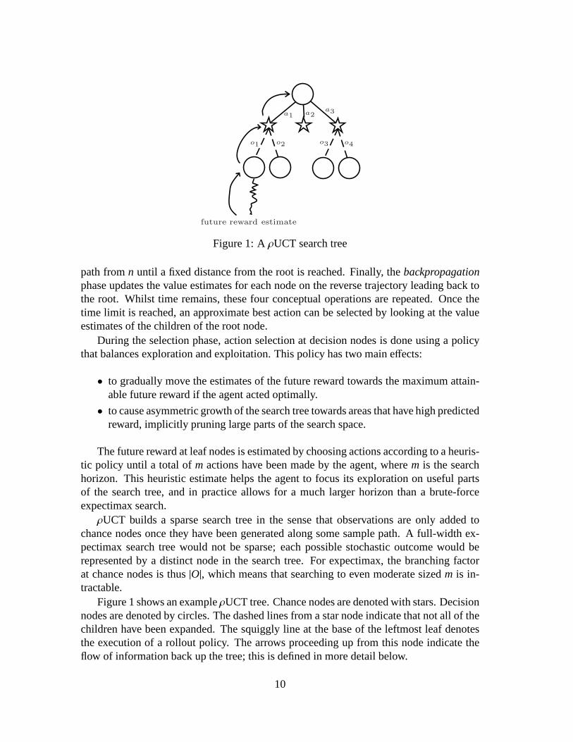
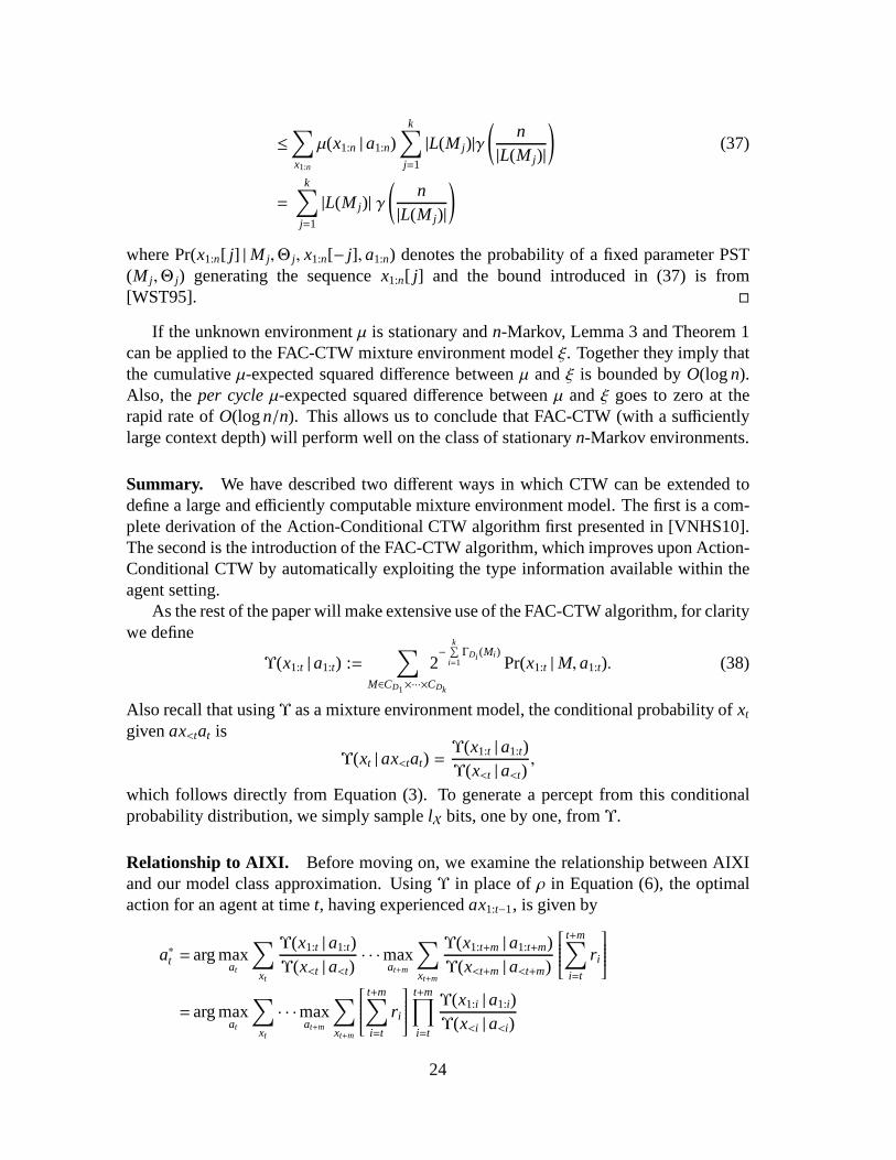
Overview. ρUCT is a best-first Monte-Carlo Tree Search technique that iteratively con-structs a search tree in memory. The tree is composed of two interleaved types of nodes:decision nodes and chance nodes. These correspond to the alternating max and sum op-erations in the expectimax operation. Each node in the tree corresponds to a historyh. Ifh ends with an action, it is a chance node; ifh ends with an observation-reward pair, it isa decision node. Each node contains a statistical estimate of the future reward.
Initially, the tree starts with a single decision node containing |A| children. Much likeexisting MCTS methods [CWU+08], there are four conceptual phases to a single iterationof ρUCT. The first is theselectionphase, where the search tree is traversed from the rootnode to an existing leaf chance noden. The second is theexpansionphase, where a newdecision node is added as a child ton. The third is thesimulationphase, where a rolloutpolicy in conjunction with the environment modelρ is used to sample a possible future
9
a1a2
a3
o1 o2 o3 o4
future reward estimate
Figure 1: AρUCT search tree
path fromn until a fixed distance from the root is reached. Finally, thebackpropagationphase updates the value estimates for each node on the reverse trajectory leading back tothe root. Whilst time remains, these four conceptual operations are repeated. Once thetime limit is reached, an approximate best action can be selected by looking at the valueestimates of the children of the root node.
During the selection phase, action selection at decision nodes is done using a policythat balances exploration and exploitation. This policy has two main effects:
• to gradually move the estimates of the future reward towardsthe maximum attain-able future reward if the agent acted optimally.
• to cause asymmetric growth of the search tree towards areas that have high predictedreward, implicitly pruning large parts of the search space.
The future reward at leaf nodes is estimated by choosing actions according to a heuris-tic policy until a total ofm actions have been made by the agent, wherem is the searchhorizon. This heuristic estimate helps the agent to focus its exploration on useful partsof the search tree, and in practice allows for a much larger horizon than a brute-forceexpectimax search.ρUCT builds a sparse search tree in the sense that observations are only added to
chance nodes once they have been generated along some samplepath. A full-width ex-pectimax search tree would not be sparse; each possible stochastic outcome would berepresented by a distinct node in the search tree. For expectimax, the branching factorat chance nodes is thus|O|, which means that searching to even moderate sizedm is in-tractable.
Figure 1 shows an exampleρUCT tree. Chance nodes are denoted with stars. Decisionnodes are denoted by circles. The dashed lines from a star node indicate that not all of thechildren have been expanded. The squiggly line at the base ofthe leftmost leaf denotesthe execution of a rollout policy. The arrows proceeding up from this node indicate theflow of information back up the tree; this is defined in more detail below.
10

Action Selection at Decision Nodes. A decision node will always contain|A| distinctchildren, all of whom are chance nodes. Associated with eachdecision node representinga particular historyh will be a value function estimate,V(h). During the selection phase,a child will need to be picked for further exploration. Action selection in MCTS poses aclassic exploration/exploitation dilemma. On one hand we need to allocate enoughvisitsto all children to ensure that we have accurate estimates forthem, but on the other handwe need to allocate enough visits to the maximal action to ensure convergence of the nodeto the value of the maximal child node.
Like UCT, ρUCT recursively uses the UCB policy [Aue02] from then-armed banditsetting at each decision node to determine which action needs further exploration. Al-though the uniform logarithmic regret bound no longer carries across from the banditsetting, the UCB policy has been shown to work well in practice in complex domainssuch as computer Go [GW06] and General Game Playing [FB08]. This policy has theadvantage of ensuring that at each decision node, every action eventually gets exploredan infinite number of times, with the best action being selected exponentially more oftenthan actions of lesser utility.
Definition 5. The visit count T(h) of a decision node h is the number of times h has beensampled by theρUCT algorithm. The visit count of the chance node found by takingaction a at h is defined similarly, and is denoted by T(ha).
Definition 6. Suppose m is the remaining search horizon and each instantaneous rewardis bounded in the interval[α, β]. Given a node representing a history h in the search tree,the action picked by the UCB action selection policy is:
aUCB(h) := arg maxa∈A
1m(β−α) V(ha) +C
√
log(T(h))T(ha) if T (ha) > 0;
∞ otherwise,(14)
where C∈ R is a positive parameter that controls the ratio of exploration to exploitation.If there are multiple maximal actions, one is chosen uniformly at random.
Note that we need a linear scaling ofV(ha) in Definition 6 because the UCB policy isonly applicable for rewards confined to the [0, 1] interval.
Chance Nodes. Chance nodes follow immediately after an action is selectedfrom adecision node. Each chance nodeha following a decision nodeh contains an estimate ofthe future utility denoted byV(ha). Also associated with the chance nodeha is a densityρ(· | ha) over observation-reward pairs.
After an actiona is performed at nodeh, ρ(· | ha) is sampled once to generate the nextobservation-reward pairor. If or has not been seen before, the nodehaor is added as achild of ha.
11
Estimating Future Reward at Leaf Nodes. If a leaf decision node is encountered atdepthk < m in the tree, a means of estimating the future reward for the remainingm− ktime steps is required. MCTS methods use a heuristic rolloutpolicy Π to estimate thesum of future rewards
∑mi=k r i. This involves sampling an actiona from Π(h), sampling
a perceptor from ρ(· | ha), appendingaor to the current historyh and then repeating thisprocess until the horizon is reached. This procedure is described in Algorithm 4. A naturalbaseline policy isΠrandom, which chooses an action uniformly at random at each time step.
As the number of simulations tends to infinity, the structureof theρUCT search treeconverges to the full depthm expectimax tree. Once this occurs, the rollout policy isno longer used byρUCT. This implies that the asymptotic value function estimates ofρUCT are invariant to the choice ofΠ. In practice, when time is limited, not enoughsimulations will be performed to grow the full expectimax tree. Therefore, the choice ofrollout policy plays an important role in determining the overall performance ofρUCT.Methods for learningΠ online are discussed as future work in Section 9. Unless otherwisestated, all of our subsequent results will useΠrandom.
Reward Backup. After the selection phase is completed, a path of nodesn1n2 . . .nk,k ≤ m, will have been traversed from the root of the search treen1 to some leafnk. Foreach 1≤ j ≤ k, the statistics maintained for historyhnj associated with noden j will beupdated as follows:
V(hnj )←T(hnj )
T(hnj ) + 1V(hnj ) +
1T(hnj ) + 1
m∑
i= j
r i (15)
T(hnj )← T(hnj ) + 1 (16)
Equation (15) computes the mean return. Equation (16) increments the visit counter. Notethat the same backup operation is applied to both decision and chance nodes.
Pseudocode. The pseudocode of theρUCT algorithm is now given.After a percept has been received, Algorithm 1 is invoked to determine an approximate
best action. Asimulationcorresponds to a single call to Sample from Algorithm 1. Byperforming a number of simulations, a search treeΨwhose root corresponds to the currenthistoryh is constructed. This tree will contain estimatesVm
ρ (ha) for eacha ∈ A. Oncethe available thinking time is exceeded, a maximising action a∗h := arg maxa∈A Vm
ρ (ha)is retrieved by BestAction. Importantly, Algorithm 1 isanytime, meaning that an ap-proximate best action is always available. This allows the agent to effectively utilise allavailable computational resources for each decision.
For simplicity of exposition, Initialise can be understood to simply clear the entiresearch treeΨ. In practice, it is possible to carry across information from one time step toanother. IfΨt is the search tree obtained at the end of timet, andaor is the agent’s actualaction and experience at timet, then we can keep the subtree rooted at nodeΨt(hao) inΨt and make that the search treeΨt+1 for use at the beginning of the next time step. Theremainder of the nodes inΨt can then be deleted.
12

Algorithm 1 ρUCT(h,m)Require: A historyhRequire: A search horizonm∈ N
1: Initialise(Ψ)2: repeat3: Sample(Ψ, h,m)4: until out of time5: return BestAction(Ψ, h)
Algorithm 2 describes the recursive routine used to sample asingle future trajectory.It uses the SelectAction routine to choose moves at decision nodes, and invokes the Roll-out routine at unexplored leaf nodes. The Rollout routine picks actions according to therollout policyΠ until the (remaining) horizon is reached, returning the accumulated re-ward. After a complete trajectory of lengthm is simulated, the value estimates are updatedfor each node traversed as per Section 4. Notice that the recursive calls on Lines 6 and 11append the most recent percept or action to the history argument.
Algorithm 2 Sample(Ψ, h,m)Require: A search treeΨRequire: A historyhRequire: A remaining search horizonm∈ N
1: if m= 0 then2: return 03: else ifΨ(h) is a chance nodethen4: Generate (o, r) from ρ(or | h)5: Create nodeΨ(hor) if T(hor) = 06: reward← r + Sample(Ψ, hor,m− 1)7: else if T(h) = 0 then8: reward← Rollout(h,m)9: else
10: a← SelectAction(Ψ, h)11: reward← Sample(Ψ, ha,m)12: end if13: V(h)← 1
T(h)+1[reward+ T(h)V(h)]14: T(h)← T(h) + 115: return reward
The action chosen by SelectAction is specified by the UCB policy described in Def-inition 6. If the selected child has not been explored before, a new node is added to thesearch tree. The constantC is a parameter that is used to control the shape of the searchtree; lower values ofC create deep, selective search trees, whilst higher values lead toshorter, bushier trees. UCB automatically focuses attention on the best looking action in
13

such a way that the sample estimateVρ(h) converges toVρ(h), whilst still exploring alter-nate actions sufficiently often to guarantee that the best action will be eventually found.
Algorithm 3 SelectAction(Ψ, h)Require: A search treeΨRequire: A historyhRequire: An exploration/exploitation constantC
1: U = {a ∈ A : T(ha) = 0}2: if U , {} then3: Pick a ∈ U uniformly at random4: Create nodeΨ(ha)5: return a6: else7: return arg max
a∈A
{
1m(β−α)V(ha) +C
√
log(T(h))T(ha)
}
8: end if
Algorithm 4 Rollout(h,m)Require: A historyhRequire: A remaining search horizonm∈ NRequire: A rollout functionΠ
1: reward← 02: for i = 1 to mdo3: Generatea fromΠ(h)4: Generate (o, r) from ρ(or | ha)5: reward← reward+ r6: h← haor7: end for8: return reward
Consistency ofρUCT. Let µ be the true underlying environment. We now establish thelink between the expectimax valueVm
µ (h) and its estimateVmµ (h) computed by theρUCT
algorithm.[KS06] show that with an appropriate choice ofC, the UCT algorithm is consistent
in finite horizon MDPs. By interpreting histories as Markov states, our general agentproblem reduces to a finite horizon MDP. This means that the results of [KS06] are nowdirectly applicable. Restating the main consistency result in our notation, we have
∀ǫ∀h limT(h)→∞
Pr(
|Vmµ (h) − Vm
µ (h)| ≤ ǫ)
= 1, (17)
14
that is,Vmµ (h)→ Vm
µ (h) with probability 1. Furthermore, the probability that a suboptimalaction (with respect toVm
µ (·)) is picked byρUCT goes to zero in the limit. Details of thisanalysis can be found in [KS06].
Parallel Implementation of ρUCT. As a Monte-Carlo Tree Search routine, Algorithm1 can be easily parallelised. The main idea is to concurrently invoke the Sample routinewhilst providing appropriate locking mechanisms for the interior nodes of the search tree.A highly scalable parallel implementation is beyond the scope of the paper, but it is worthnoting that ideas applicable to high performance Monte-Carlo Go programs [CWH08]can be easily transferred to our setting.
5 Model Class Approximation using Context TreeWeighting
We now turn our attention to the construction of an efficient mixture environment modelsuitable for the general reinforcement learning problem. If computation were not an issue,it would be sufficient to first specify a large model classM, and then use Equations (8)or (3) for online prediction. The problem with this approachis that at leastO(|M|) timeis required to process each new piece of experience. This is simply too slow for theenormous model classes required by general agents. Instead, this section will describehow to predict inO(log log|M|) time, using a mixture environment model constructedfrom an adaptation of the Context Tree Weighting algorithm.
Context Tree Weighting. Context Tree Weighting (CTW) [WST95, WST97] is an effi-cient and theoretically well-studied binary sequence prediction algorithm that works wellin practice [BEYY04]. It is an online Bayesian model averaging algorithm that computes,at each time pointt, the probability
Pr(y1:t) =∑
M
Pr(M) Pr(y1:t |M), (18)
wherey1:t is the binary sequence seen so far,M is a prediction suffix tree [Ris83, RST96],Pr(M) is the prior probability ofM, and the summation is overall prediction suffix treesof bounded depthD. This is a huge class, covering allD-order Markov processes. A naıvecomputation of (18) takes timeO(22D
); using CTW, this computation requires onlyO(D)time. In this section, we outline two ways in which CTW can be generalised to computeprobabilities of the form
Pr(x1:t | a1:t) =∑
M
Pr(M) Pr(x1:t |M, a1:t), (19)
wherex1:t is a percept sequence,a1:t is an action sequence, andM is a prediction suffixtree as in (18). These generalisations will allow CTW to be used as a mixture environmentmodel.
15

Krichevsky-Trofimov Estimator. We start with a brief review of the KT estimator[KT81] for Bernoulli distributions. Given a binary stringy1:t with a zeros andb ones,the KT estimate of the probability of the next symbol is as follows:
Prkt(Yt+1 = 1 | y1:t) :=b+ 1/2
a+ b+ 1(20)
Prkt(Yt+1 = 0 | y1:t) := 1− Prkt(Yt+1 = 1 | y1:t). (21)
The KT estimator is obtained via a Bayesian analysis by putting an uninformative (JeffreysBeta(1/2,1/2)) prior Pr(θ) ∝ θ−1/2(1 − θ)−1/2 on the parameterθ ∈ [0, 1] of the Bernoullidistribution. From (20)-(21), we obtain the following expression for the block probabilityof a string:
Prkt(y1:t) = Prkt(y1 | ǫ)Prkt(y2 | y1) · · ·Prkt(yt | y<t)
=∫
θb(1− θ)a Pr(θ) dθ.
Since Prkt(s) depends only on the number of zerosas and onesbs in a strings, if we let0a1b denote a string witha zeroes andb ones, then we have
Prkt(s) = Prkt(0as1bs) =
1/2(1+ 1/2) · · · (as− 1/2)1/2(1+ 1/2) · · · (bs− 1/2)(as+ bs)!
. (22)
We write Prkt(a, b) to denote Prkt(0a1b) in the following. The quantity Prkt(a, b) can beupdated incrementally [WST95] as follows:
Prkt(a+ 1, b) =a+ 1/2
a+ b+ 1Prkt(a, b) (23)
Prkt(a, b+ 1) =b+ 1/2
a+ b+ 1Prkt(a, b), (24)
with the base case being Prkt(0, 0) = 1.
Prediction Suffix Trees. We next describe prediction suffix trees, which are a form ofvariable-order Markov models.
In the following, we work with binary trees where all the leftedges are labeled 1 andall the right edges are labeled 0. Each node in such a binary treeM can be identified by astring in{0, 1}∗ as follows:ǫ represents the root node ofM; and ifn ∈ {0, 1}∗ is a node inM, thenn1 andn0 represent the left and right child of noden respectively. The set ofM’sleaf nodesL(M) ⊂ {0, 1}∗ form a complete prefix-free set of strings. Given a binary stringy1:t such thatt ≥ the depth ofM, we defineM(y1:t) := ytyt−1 . . . yt′ , wheret′ ≤ t is the(unique) positive integer such thatytyt−1 . . . yt′ ∈ L(M). In other words,M(y1:t) representsthe suffix of y1:t that occurs in treeM.
Definition 7. A prediction suffix tree (PST) is a pair(M,Θ), where M is a binary tree andassociated with each leaf node l in M is a probability distribution over{0, 1} parametrisedbyθl ∈ Θ. We call M the model of the PST andΘ the parameter of the PST, in accordancewith the terminology of [WST95].
16
θ1 = 0.1
◦1
������
�� 0
��??
????
?
θ01 = 0.3
◦1
������
�� 0
��??
????
θ00 = 0.5
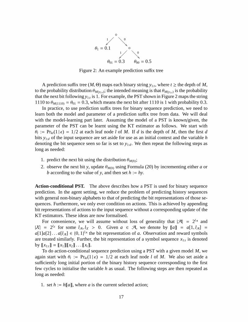
Figure 2: An example prediction suffix tree
A prediction suffix tree (M,Θ) maps each binary stringy1:t, wheret ≥ the depth ofM,to the probability distributionθM(y1:t); the intended meaning is thatθM(y1:t) is the probabilitythat the next bit followingy1:t is 1. For example, the PST shown in Figure 2 maps the string1110 toθM(1110)= θ01 = 0.3, which means the next bit after 1110 is 1 with probability 0.3.
In practice, to use prediction suffix trees for binary sequence prediction, we need tolearn both the model and parameter of a prediction suffix tree from data. We will dealwith the model-learning part later. Assuming the model of a PST is known/given, theparameter of the PST can be learnt using the KT estimator as follows. We start withθl := Prkt(1 | ǫ) = 1/2 at each leaf nodel of M. If d is the depth ofM, then the firstdbits y1:d of the input sequence are set aside for use as an initial context and the variablehdenoting the bit sequence seen so far is set toy1:d. We then repeat the following steps aslong as needed:
1. predict the next bit using the distributionθM(h);
2. observe the next bity, updateθM(h) using Formula (20) by incrementing eithera orb according to the value ofy, and then seth := hy.
Action-conditional PST. The above describes how a PST is used for binary sequenceprediction. In the agent setting, we reduce the problem of predicting history sequenceswith general non-binary alphabets to that of predicting thebit representations of those se-quences. Furthermore, we only ever condition on actions. This is achieved by appendingbit representations of actions to the input sequence without a corresponding update of theKT estimators. These ideas are now formalised.
For convenience, we will assume without loss of generality that |A| = 2lA and|X| = 2lX for some lA, lX > 0. Given a ∈ A, we denote by~a� = a[1, lA] =a[1]a[2] . . .a[lA] ∈ {0, 1}lA the bit representation ofa. Observation and reward symbolsare treated similarly. Further, the bit representation of asymbol sequencex1:t is denotedby ~x1:t� = ~x1�~x2� . . . ~xt�.
To do action-conditional sequence prediction using a PST with a given modelM, weagain start withθl := Prkt(1 | ǫ) = 1/2 at each leaf nodel of M. We also set aside asufficiently long initial portion of the binary history sequencecorresponding to the firstfew cycles to initialise the variableh as usual. The following steps are then repeated aslong as needed:
1. seth := h~a�, wherea is the current selected action;
17
2. for i := 1 to lX do
(a) predict the next bit using the distributionθM(h);
(b) observe the next bitx[i], updateθM(h) using Formula (20) according to thevalue ofx[i], and then seth := hx[i].
Let M be the model of a prediction suffix tree,a1:t ∈ At an action sequence,x1:t ∈ X
t
an observation-reward sequence, andh := ~ax1:t�. For each noden in M, definehM,n by
hM,n := hi1hi2 · · ·hik (25)
where 1 ≤ i1 < i2 < · · · < ik ≤ t and, for eachi, i ∈ {i1, i2, . . . ik} iff hi is anobservation-reward bit andn is a prefix of M(h1:i−1). In other words,hM,n consists ofall the observation-reward bits with contextn. Thus we have the following expression forthe probability ofx1:t givenM anda1:t:
Pr(x1:t |M, a1:t) =t
∏
i=1
Pr(xi |M, ax<iai)
=
t∏
i=1
lX∏
j=1
Pr(xi[ j] |M, ~ax<iai�xi[1, j − 1])
=∏
n∈L(M)
Prkt(hM,n). (26)
The last step follows by grouping the individual probability terms according to thenoden ∈ L(M) in which each bit falls and then observing Equation (22). The above dealswith action-conditional prediction using a single PST. We now show how we can performefficient action-conditional prediction using a Bayesian mixture of PSTs. First we specifya prior over PST models.
A Prior on Models of PSTs. Our prior Pr(M) := 2−ΓD(M) is derived from a natural prefixcoding of the tree structure of a PST. The coding scheme worksas follows: given a modelof a PST of maximum depthD, a pre-order traversal of the tree is performed. Each timean internal node is encountered, we write down 1. Each time a leaf node is encountered,we write a 0 if the depth of the leaf node is less thanD; otherwise we write nothing. Forexample, ifD = 3, the code for the model shown in Figure 2 is 10100; ifD = 2, the codefor the same model is 101. The costΓD(M) of a modelM is the length of its code, whichis given by the number of nodes inM minus the number of leaf nodes inM of depthD.One can show that
∑
M∈CD
2−ΓD(M) = 1,
whereCD is the set of all models of prediction suffix trees with depth at mostD; i.e. theprefix code is complete. We remark that the above is another way of describing the codingscheme in [WST95]. Note that this choice of prior imposes an Ockham-like penalty onlarge PST structures.
18

ǫ
ǫ1
������
� 0
��??
???
ǫ1
������
� 0
��??
???
ǫ ǫ
ǫ1
������
� 0
��??
???
ǫ ǫ
ǫ1
������
�� 0
��??
????
01
������
�� 0
��??
????
ǫ 0
01����
��� 0
��??
????
ǫ ǫ
ǫ1
������
�� 0
��??
????
011
������
�� 0
��??
???
ǫ 0
011
������
� 0
��??
????
1
Figure 3: A depth-2 context tree (left); trees after processing two bits (middle and right)
Context Trees. The following data structure is a key ingredient of the Action-Conditional CTW algorithm.
Definition 8. A context tree of depth D is a perfect binary tree of depth D such thatattached to each node (both internal and leaf) is a probability on{0, 1}∗.
The node probabilities in a context tree are estimated from data by using a KT estima-tor at each node. The process to update a context tree with a history sequence is similarto a PST, except that:
1. the probabilities at each node in the path from the root to aleaf traversed by anobserved bit are updated; and
2. we maintain block probabilities using Equations (22) to (24) instead of conditionalprobabilities.
This process can be best understood with an example. Figure 3(left) shows a contexttree of depth two. For expositional reasons, we show binary sequences at the nodes;the node probabilities are computed from these. Initially,the binary sequence at eachnode is empty. Suppose 1001 is the history sequence. Settingaside the first two bits10 as an initial context, the tree in the middle of Figure 3 shows what we have afterprocessing the third bit 0. The tree on the right is the tree wehave after processingthe fourth bit 1. In practice, we of course only have to store the counts of zeros andones instead of complete subsequences at each node because,as we saw earlier in (22),Prkt(s) = Prkt(as, bs). Since the node probabilities are completely determined by the inputsequence, we shall henceforth speak unambiguously aboutthecontext tree after seeing asequence.
The context tree of depthD after seeing a sequenceh has the following importantproperties:
1. the model of every PST of depth at mostD can be obtained from the context treeby pruning off appropriate subtrees and treating them as leaf nodes;
2. the block probability ofh as computed by each PST of depth at mostD can beobtained from the node probabilities of the context tree viaEquation (26).
These properties, together with an application of the distributive law, form the basis of thehighly efficient Action Conditional CTW algorithm. We now formalise these insights.
19

Weighted Probabilities. The weighted probabilityPnw of each noden in the context tree
T after seeingh := ~ax1:t� is defined inductively as follows:
Pnw :=
Prkt(hT,n) if n is a leaf node;12 Prkt(hT,n) + 1
2Pn0w × Pn1
w otherwise,(27)
wherehT,n is as defined in (25).
Lemma 2 ([WST95]). Let T be the depth-D context tree after seeing h:= ~ax1:t�. Foreach node n in T at depth d, we have
Pnw =
∑
M∈CD−d
2−ΓD−d(M)∏
n′∈L(M)
Prkt(hT,nn′). (28)
Proof. The proof proceeds by induction ond. The statement is clearly true for the leafnodes at depthD. Assume now the statement is true for all nodes at depthd + 1, where0 ≤ d < D. Consider a noden at depthd. Lettingd = D − d, we have
Pnw =
12
Prkt(hT,n) +12
Pn0w Pn1
w
=12
Prkt(hT,n) +12
∑
M∈Cd+1
2−Γd+1(M)∏
n′∈L(M)
Prkt(hT,n0n′)
∑
M∈Cd+1
2−Γd+1(M)∏
n′∈L(M)
Prkt(hT,n1n′)
=12
Prkt(hT,n) +∑
M1∈Cd+1
∑
M2∈Cd+1
2−(Γd+1(M1)+Γd+1(M2)+1)
∏
n′∈L(M1)
Prkt(hT,n0n′)
∏
n′∈L(M2)
Prkt(hT,n1n′)
=12
Prkt(hT,n) +∑
M1M2∈Cd
2−Γd(M1M2)∏
n′∈L(M1M2)
Prkt(hT,nn′)
=∑
M∈CD−d
2−ΓD−d(M)∏
n′∈L(M)
Prkt(hT,nn′),
whereM1M2 denotes the tree inCd whose left and right subtrees areM1 andM2 respec-tively. �
Action Conditional CTW as a Mixture Environment Model. A corollary of Lemma2 is that at the root nodeǫ of the context treeT after seeingh := ~ax1:t�, we have
Pǫw =∑
M∈CD
2−ΓD(M)∏
l∈L(M)
Prkt(hT,l) (29)
=∑
M∈CD
2−ΓD(M)∏
l∈L(M)
Prkt(hM,l) (30)
=∑
M∈CD
2−ΓD(M) Pr(x1:t |M, a1:t), (31)
20

where the last step follows from Equation (26). Equation (31) shows that the quantitycomputed by the Action-Conditional CTW algorithm is exactly a mixture environmentmodel. Note that the conditional probability is always defined, as CTW assigns a non-zero probability to any sequence. To sample from this conditional probability, we simplysample the individual bits ofxt one by one.
In summary, to do prediction using Action-Conditional CTW,we set aside a suffi-ciently long initial portion of the binary history sequencecorresponding to the first fewcycles to initialise the variableh and then repeat the following steps as long as needed:
1. seth := h~a�, wherea is the current selected action;
2. for i := 1 to lX do
(a) predict the next bit using the weighted probabilityPǫw;
(b) observe the next bitx[i], update the context tree usingh andx[i], calculate thenew weighted probabilityPǫw, and then seth := hx[i].
Incorporating Type Information. One drawback of the Action-Conditional CTW al-gorithm is the potential loss of type information when mapping a history string to itsbinary encoding. This type information may be needed for predicting well in some do-mains. Although it is always possible to choose a binary encoding scheme so that thetype information can be inferred by a depth limited context tree, it would be desirable toremove this restriction so that our agent can work with arbitrary encodings of the perceptspace.
One option would be to define an action-conditional version of multi-alphabet CTW[TSW93], with the alphabet consisting of the entire perceptspace. The downside of thisapproach is that we then lose the ability to exploit the structure within each percept. Thiscan be critical when dealing with large observation spaces,as noted by [McC96]. The keydifference between his U-Tree and USM algorithms is that the former could discriminatebetween individual components within an observation, whereas the latter worked only atthe symbol level. As we shall see in Section 7, this property can be helpful when dealingwith larger problems.
Fortunately, it is possible to get the best of both worlds. Wenow describe a techniquethat incorporates type information whilst still working atthe bit level. The trick is tochain togetherk := lX action conditional PSTs, one for each bit of the percept space, withappropriately overlapping binary contexts. More precisely, given a historyh, the contextfor theith PST is the most recentD+ i −1 bits of the bit-level history string~h�x[1, i −1].To ensure that each percept bit is dependent on the same portion of h, D + i − 1 (insteadof only D) bits are used. Thus if we denote the PST model for theith bit in a perceptx byMi, and the joint model byM, we now have:
Pr(x1:t |M, a1:t) =t
∏
i=1
Pr(xi |M, ax<iai)
21

=
t∏
i=1
k∏
j=1
Pr(xi[ j] |M j, ~ax<iai�xi[1, j − 1]) (32)
=
k∏
j=1
Pr(x1:t[ j] |M j, x1:t[− j], a1:t)
wherex1:t[i] denotesx1[i]x2[i] . . . xt[i], x1:t[−i] denotesx1[−i]x2[−i] . . . xt[−i], with xt[− j]denotingxt[1] . . . xt[ j − 1]xt[ j + 1] . . . xt[k]. The last step follows by swapping the twoproducts in (32) and using the above notation to refer to the product of probabilities of thejth bit in each perceptxi, for 1≤ i ≤ t.
We next place a prior on the space of factored PST modelsM ∈ CD × · · · ×CD+k−1 byassuming that each factor is independent, giving
Pr(M) = Pr(M1, . . . ,Mk) =k
∏
i=1
2−ΓDi (Mi ) = 2−
k∑
i=1ΓDi (Mi )
,
whereDi := D + i − 1. This induces the following mixture environment model
ξ(x1:t | a1:t) :=∑
M∈CD1×···×CDk
2−
k∑
i=1ΓDi (Mi )
Pr(x1:t |M, a1:t). (33)
This can now be rearranged into a product of efficiently computable mixtures, since
ξ(x1:t | a1:t) =∑
M1∈CD1
· · ·∑
Mk∈CDk
2−
k∑
i=1ΓDi (Mi )
k∏
j=1
Pr(x1:t[ j] |M j, x1:t[− j], a1:t)
=
k∏
j=1
∑
M j∈CD j
2−ΓD j (M j ) Pr(x1:t[ j] |M j, x1:t[− j], a1:t)
. (34)
Note that for each factor within Equation (34), a result analogous to Lemma 2 can beestablished by appropriately modifying Lemma 2’s proof to take into account that nowonly one bit per percept is being predicted. This leads to thefollowing scheme for incre-mentally maintaining Equation (33):
1. Initialiseh← ǫ, t ← 1. Createk context trees.
2. Determine actionat. Seth← hat.
3. Receivext. For each bitxt[i] of xt, update theith context tree withxt[i] using historyhx[1, i − 1] and recomputePǫw using Equation (27).
4. Seth← hxt, t ← t + 1. Goto 2.
We will refer to this technique as Factored Action-Conditional CTW, or the FAC-CTWalgorithm for short.
22

Convergence to the True Environment. We now show that FAC-CTW performs wellin the class of stationaryn-Markov environments. Importantly, this includes the class ofMarkov environments used in state-based reinforcement learning, where the most recentaction/observation pair (at, xt−1) is a sufficient statistic for the prediction ofxt.
Definition 9. Given n∈ N, an environmentµ is said to be n-Markov if for all t> n, forall a1:t ∈ A
t, for all x1:t ∈ Xt and for all h∈ (A×X)t−n−1 ×A
µ(xt | ax<tat) = µ(xt | hxt−naxt−n+1:t−1at). (35)
Furthermore, an n-Markov environment is said to be stationary if for all ax1:nan+1 ∈ (A×X)n × A, for all h, h′ ∈ (A×X)∗,
µ(· | hax1:nan+1) = µ(· | h′ax1:nan+1). (36)
It is easy to see that any stationaryn-Markov environment can be represented as aproduct of sufficiently large, fixed parameter PSTs. Theorem 1 states that the predictionsmade by a mixture environment model only converge to those ofthe true environmentwhen the model class contains a model sufficiently close to the true environment. How-ever, nostationary n-Markov environment model is contained within the model class ofFAC-CTW, since each model updates the parameters for its KT-estimators as more datais seen. Fortunately, this is not a problem, since this updating produces models that aresufficiently close to any stationaryn-Markov environment for Theorem 1 to be meaning-ful.
Lemma 3. IfM is the model class used byFAC-CTWwith a context depth D,µ is an en-vironment expressible as a product of k:= lX fixed parameter PSTs(M1,Θ1), . . . , (Mk,Θk)of maximum depth D andρ(· | a1:n) ≡ Pr(· | (M1, . . . ,Mk), a1:n) ∈ M then for all n∈ N, forall a1:n ∈ A
n,
D1:n(µ || ρ) ≤k
∑
j=1
|L(M j)| γ
(
n|L(M j)|
)
where
γ(z) :=
{
z for 0 ≤ z< 112 logz+ 1 for z≥ 1.
Proof. For alln ∈ N, for all a1:n ∈ An,
D1:n(µ || ρ) =∑
x1:n
µ(x1:n | a1:n) lnµ(x1:n | a1:n)ρ(x1:n | a1:n)
=∑
x1:n
µ(x1:n | a1:n) ln
∏kj=1 Pr(x1:n[ j] |M j,Θ j, x1:n[− j], a1:n)∏k
j=1 Pr(x1:n[ j] |M j, x1:n[− j], a1:n)
=∑
x1:n
µ(x1:n | a1:n)k
∑
j=1
lnPr(x1:n[ j] |M j,Θ j, x1:n[− j], a1:n)
Pr(x1:n[ j] |M j, x1:n[− j], a1:n)
23
≤∑
x1:n
µ(x1:n | a1:n)k
∑
j=1
|L(M j)|γ
(
n|L(M j)|
)
(37)
=
k∑
j=1
|L(M j)| γ
(
n|L(M j)|
)
where Pr(x1:n[ j] |M j,Θ j, x1:n[− j], a1:n) denotes the probability of a fixed parameter PST(M j ,Θ j) generating the sequencex1:n[ j] and the bound introduced in (37) is from[WST95]. �
If the unknown environmentµ is stationary andn-Markov, Lemma 3 and Theorem 1can be applied to the FAC-CTW mixture environment modelξ. Together they imply thatthe cumulativeµ-expected squared difference betweenµ andξ is bounded byO(logn).Also, theper cycleµ-expected squared difference betweenµ andξ goes to zero at therapid rate ofO(logn/n). This allows us to conclude that FAC-CTW (with a sufficientlylarge context depth) will perform well on the class of stationaryn-Markov environments.
Summary. We have described two different ways in which CTW can be extended todefine a large and efficiently computable mixture environment model. The first is acom-plete derivation of the Action-Conditional CTW algorithm first presented in [VNHS10].The second is the introduction of the FAC-CTW algorithm, which improves upon Action-Conditional CTW by automatically exploiting the type information available within theagent setting.
As the rest of the paper will make extensive use of the FAC-CTWalgorithm, for claritywe define
Υ(x1:t | a1:t) :=∑
M∈CD1×···×CDk
2−
k∑
i=1ΓDi (Mi )
Pr(x1:t |M, a1:t). (38)
Also recall that usingΥ as a mixture environment model, the conditional probability of xt
givenax<tat is
Υ(xt | ax<tat) =Υ(x1:t | a1:t)Υ(x<t | a<t)
,
which follows directly from Equation (3). To generate a percept from this conditionalprobability distribution, we simply samplelX bits, one by one, fromΥ.
Relationship to AIXI. Before moving on, we examine the relationship between AIXIand our model class approximation. UsingΥ in place ofρ in Equation (6), the optimalaction for an agent at timet, having experiencedax1:t−1, is given by
a∗t = arg maxat
∑
xt
Υ(x1:t | a1:t)Υ(x<t | a<t)
· · ·maxat+m
∑
xt+m
Υ(x1:t+m | a1:t+m)Υ(x<t+m | a<t+m)
t+m∑
i=t
r i
= arg maxat
∑
xt
· · ·maxat+m
∑
xt+m
t+m∑
i=t
r i
t+m∏
i=t
Υ(x1:i | a1:i)Υ(x<i | a<i)
24

= arg maxat
∑
xt
· · ·maxat+m
∑
xt+m
t+m∑
i=t
r i
Υ(x1:t+m | a1:t+m)Υ(x<t | a<t)
= arg maxat
∑
xt
· · ·maxat+m
∑
xt+m
t+m∑
i=t
r i
Υ(x1:t+m | a1:t+m)
= arg maxat
∑
xt
· · ·maxat+m
∑
xt+m
t+m∑
i=t
r i
∑
M∈CD1×···×CDk
2−
k∑
i=1ΓDi (Mi )
Pr(x1:t+m |M, a1:t+m). (39)
Contrast (39) now with Equation (11) which we reproduce here:
a∗t = arg maxat
∑
xt
. . .maxat+m
∑
xt+m
t+m∑
i=t
r i
∑
ρ∈M
2−K(ρ)ρ(x1:t+m | a1:t+m), (40)
whereM is the class of all enumerable chronological semimeasures,andK(ρ) denotes theKolmogorov complexity ofρ. The two expressions share a prior that enforces a bias to-wards simpler models. The main difference is in the subexpression describing the mixtureover the model class. AIXI uses a mixture over all enumerablechronological semimea-sures. This is scaled down to a (factored) mixture of prediction suffix trees in our setting.Although the model class used in AIXI is completely general,it is also incomputable. Ourapproximation has restricted the model class to gain the desirable computational proper-ties of FAC-CTW.
6 Putting it All Together
Our approximate AIXI agent, MC-AIXI(fac-ctw), is realised by instantiating theρUCTalgorithm withρ = Υ. Some additional properties of this combination are now discussed.
Convergence of Value. We now show that usingΥ in place of the true environmentµ in the expectimax operation leads to good behaviour whenµ is both stationary andn-Markov. This result combines Lemma 3 with an adaptation of [Hut05, Thm.5.36]. Forthis analysis, we assume that the instantaneous rewards arenon-negative (with no loss ofgenerality), FAC-CTW is used with a sufficiently large context depth, the maximum lifeof the agentb ∈ N is fixed and that a bounded planning horizonmt := min(H, b− t + 1) isused at each timet, with H ∈ N specifying the maximum planning horizon.
Theorem 2. Using theFAC-CTW algorithm, for every policyπ, if the true environmentµ is expressible as a product of k PSTs(M1,Θ1), . . . , (Mk,Θk), for all b ∈ N, we have
b∑
t=1
Ex<t∼µ
[
(
vmtΥ
(π, ax<t) − vmtµ (π, ax<t)
)2]
≤ 2H3r2max
k∑
i=1
ΓDi (Mi) +k
∑
j=1
|L(M j)| γ
(
b|L(M j)|
)
where rmax is the maximum instantaneous reward,γ is as defined in Lemma 3 andvmtµ (π, ax<t) is the value of policyπ as defined in Definition 3.
25

Proof. First defineρ(xi: j | a1: j , x<i) := ρ(x1: j | a1: j)/ρ(x<i | a<i) for i < j , for any environ-ment modelρ and letat:mt be the actions chosen byπ at timest to mt. Now
∣
∣
∣vmtΥ
(π, ax<t) − vmtµ (π, ax<t)
∣
∣
∣ =
∣
∣
∣
∣
∣
∣
∣
∣
∑
xt:mt
(r t + · · · + rmt)[
Υ(xt:mt | a1:mt , x<t) − µ(xt:mt | a1:mt , x<t)]
∣
∣
∣
∣
∣
∣
∣
∣
≤∑
xt:mt
(r t + · · · + rmt)∣
∣
∣Υ(xt:mt | a1:mt , x<t) − µ(xt:mt | a1:mt , x<t)∣
∣
∣
≤ mtrmax
∑
xt:mt
∣
∣
∣Υ(xt:mt | a1:mt , x<t) − µ(xt:mt | a1:mt , x<t)∣
∣
∣
=: mtrmaxAt:mt (µ || Υ).
Applying this bound, a property of absolute distance [Hut05, Lemma 3.11] and the chainrule for KL-divergence [CT91, p. 24] gives
b∑
t=1
Ex<t∼µ
[
(
vmtΥ
(π, ax<t) − vmtµ (π, ax<t)
)2]
≤ m2t r
2max
b∑
t=1
Ex<t∼µ
[
At:mt (µ || Υ)2]
≤ 2H2r2max
b∑
t=1
Ex<t∼µ
[
Dt:mt (µ || Υ)]
= 2H2r2max
b∑
t=1
mt∑
i=t
Ex<i∼µ
[
Di:i(µ || Υ)]
≤ 2H3r2max
b∑
t=1
Ex<t∼µ
[
Dt:t(µ || Υ)]
= 2H3r2maxD1:b(µ || Υ),
whereDi: j(µ || Υ) :=∑
xi: jµ(xi: j | a1: j, x<i) ln(Υ(xi: j | a1: j , x<i)/µ(xi: j | a1: j , x<i)). The final
inequality uses the fact that any particularDi:i(µ || Υ) term appears at mostH times in thepreceding double sum. Now defineρM(· | a1:b) := Pr(· | (M1, . . . ,Mk), a1:b) and we have
D1:b(µ || Υ) =∑
x1:b
µ(x1:b | a1:b) ln
[
µ(x1:b | a1:b)ρM(x1:b | a1:b)
ρM(x1:b | a1:b)Υ(x1:b | a1:b)
]
=∑
x1:b
µ(x1:b | a1:b) lnµ(x1:b | a1:b)ρM(x1:b | a1:b)
+∑
x1:b
µ(x1:b | a1:b) lnρM(x1:b | a1:b)Υ(x1:b | a1:b)
≤ D1:b(µ ‖ ρM) +∑
x1:b
µ(x1:b | a1:b) lnρM(x1:b | a1:b)
wρM
0 ρM(x1:b | a1:b)
= D1:b(µ ‖ ρM) +k
∑
i=1
ΓDi (Mi)
wherewρM
0 := 2−
k∑
i=1ΓDi (Mi )
and the final inequality follows by dropping all butρM ’s con-tribution to Equation (38). Using Lemma 3 to boundD1:b(µ ‖ ρM) now gives the desiredresult. �
For any fixedH, Theorem 2 shows that the cumulative expected squared differenceof the true andΥ values is bounded by a term that grows at the rate ofO(logb). The
26

average expected squared difference of the two values then goes down to zero at the rateof O( logb
b ). This implies that for sufficiently largeb, the value estimates usingΥ in place ofµ converge for any fixed policyπ. Importantly, this includes the fixed horizon expectimaxpolicy with respect toΥ.
Convergence to Optimal Policy. This section presents a result forn-Markov environ-ments that are both ergodic and stationary. Intuitively, this class of environments neverallow the agent to make a mistake from which it can no longer recover. Thus in these en-vironments an agent that learns from its mistakes can hope toachieve a long-term averagereward that will approach optimality.
Definition 10. An n-Markov environmentµ is said to be ergodic if there exists a policyπ such that every sub-history s∈ (A×X)n possible inµ occurs infinitely often (withprobability1) in the history generated by an agent/environment pair(π, µ).
Definition 11. A sequence of policies{π1, π2, . . . } is said to be self optimising with respectto model classM if
1m
vmρ (πm, ǫ) −
1m
Vmρ (ǫ)→ 0 as m→∞ for all ρ ∈ M. (41)
A self optimising policy has the same long-term average expected future reward asthe optimal policy for any environment inM. In general, such policies cannot exist forall model classes. We restrict our attention to the set of stationary, ergodicn-Markovenvironments since these are what can be modeled effectively by FAC-CTW. The ergod-icity property ensures that no possible percepts are precluded due to earlier actions by theagent. The stationarity property ensures that the environment is sufficiently well behavedfor a PST to learn a fixed set of parameters.
We now prove a lemma in preparation for our main result.
Lemma 4. Any stationary, ergodic n-Markov environment can be modeled by a finite,ergodic MDP.
Proof. Given an ergodicn-Markov environmentµ, with associated action spaceA andpercept spaceX, an equivalent, finite MDP (S,A,T,R) can be constructed fromµ bydefining the state space asS := (A× X)n, the action space asA := A, the transitionprobability asTa(s, s′) := µ(o′r ′ | hsa) and the reward function asRa(s, s′) := r ′, wheres′
is the suffix formed by deleting the leftmost action/percept pair fromsao′r ′ andh is anarbitrary history from (A×X)∗. Ta(s, s′) is well defined for arbitraryhsinceµ is stationary,therefore Eq. (36) applies. Definition 10 implies that the derived MDP is ergodic. �
Theorem 3. Given a mixture environment modelξ over a model classM consisting ofa countable set of stationary, ergodic n-Markov environments, the sequence of policies{
πξ
1, πξ
2, . . .}
where
πξ
b(ax<t) := arg maxat∈A
Vb−t+1ξ (ax<tat) (42)
for 1 ≤ t ≤ b, is self-optimising with respect to model classM.
27
Proof. By applying Lemma 4 to eachρ ∈ M, an equivalent model classN of finite,ergodic MDPs can be produced. We know from [Hut05, Thm.5.38]that a sequence ofpolicies forN that is self-optimising exists. This implies the existenceof a correspondingsequence of policies forM that is self-optimising. Using [Hut05, Thm.5.29], this impliesthat the sequence of policies
{
πξ
1, πξ
2, . . .}
is self optimising. �
Theorem 3 says that by choosing a sufficiently large lifespanb, the average reward foran agent following policyπξb can be made arbitrarily close to the optimal average rewardwith respect to the true environment.
Theorem 3 and the consistency of theρUCT algorithm (17) give support to the claimthat the MC-AIXI(fac-ctw) agent is self-optimising with respect to the class of stationary,ergodic,n-Markov environments. The argument isn’t completely rigorous, since the usageof the KT-estimator implies that the model class of FAC-CTW contains an uncountablenumber of models. Our conclusion is not entirely unreasonable however. The justificationis that a countable mixture of PSTs behaving similarly to theFAC-CTW mixture can beformed by replacing each PST leaf node KT-estimator with a finely grained, discreteBayesian mixture predictor. Under this interpretation, a floating point implementation ofthe KT-estimator would correspond to a computationally feasible approximation of theabove.
The results used in the proof of Theorem 3 can be found in [Hut02b] and [LH04].An interesting direction for future work would be to investigate whether a self-optimisingresult similar to [Hut05, Thm.5.29] holds for continuous mixtures.
Computational Properties. The FAC-CTW algorithm grows each context tree datastructure dynamically. With a context depthD, there are at mostO(tD log(|O||R|)) nodesin the set of context trees aftert cycles. In practice, this is considerably less thanlog(|O||R|)2D, which is the number of nodes in a fully grown set of context trees. Thetime complexity of FAC-CTW is also impressive;O(Dmlog(|O||R|)) to generate thempercepts needed to perform a singleρUCT simulation andO(D log(|O||R|)) to processeach new piece of experience. Importantly, these quantities are not dependent ont, whichmeans that the performance of our agent does not degrade withtime. Thus it is reasonableto run our agent in an online setting for millions of cycles. Furthermore, as FAC-CTW isan exact algorithm, we do not suffer from approximation issues that plague sample basedapproaches to Bayesian learning.
Efficient Combination of FAC-CTW with ρUCT. Earlier, we showed how FAC-CTWcan be used in an online setting. An additional property however is needed for efficient usewithin ρUCT. Before Sample is invoked, FAC-CTW will have computed a set of contexttrees for a history of lengtht. After a complete trajectory is sampled, FAC-CTW will nowcontain a set of context trees for a history of lengtht+m. The original set of context treesnow needs to be restored. Saving and copying the original context trees is unsatisfactory,as is rebuilding them from scratch inO(tD log(|O||R|)) time. Luckily, the original setof context trees can be recovered efficiently by traversing the history at timet + m in
28
reverse, and performing an inverse update operation on eachof the D affected nodes inthe relevant context tree, for each bit in the sample trajectory. This takesO(Dmlog(|O||R|))time. Alternatively, a copy on write implementation can be used to modify the contexttrees during the simulation phase, with the modified copies of each context node discardedbefore Sample is invoked again.
Exploration /Exploitation in Practice. Bayesian belief updating combines well withexpectimax based planning. Agents using this combination,such as AIXI andMC-AIXI( fac-ctw), will automatically perform information gathering actions if the ex-pected reduction in uncertainty would lead to higher expected future reward. Since AIXIis a mathematical notion, it can simply take a large initial planning horizonb, e.g. itsmaximal lifespan, and then at each cyclet choose greedily with respect to Equation (1)using aremaining horizonof b− t + 1. Unfortunately in the case of MC-AIXI(fac-ctw),the situation is complicated by issues of limited computation.
In theory, the MC-AIXI(fac-ctw) agent could always perform the action recom-mended byρUCT. In practice however, performing an expectimax operation with a re-maining horizon ofb−t+1 is not feasible, even using Monte-Carlo approximation. Insteadwe use as large a fixed search horizon as we can afford computationally, and occasionallyforce exploration according to some heuristic policy. The intuition behind this choice isthat in many domains, good behaviour can be achieved by usinga small amount of plan-ning if the dynamics of the domain are known. Note that it is still possible forρUCT torecommend an exploratory action, but only if the benefits of this information can be re-alised within its limited planning horizon. Thus, a limitedamount of exploration can helpthe agent avoid local optima with respect to its present set of beliefs about the underlyingenvironment. Other online reinforcement learning algorithms such as SARSA(λ) [SB98],U-Tree [McC96] or Active-LZ [FMVRW10] employ similar such strategies.
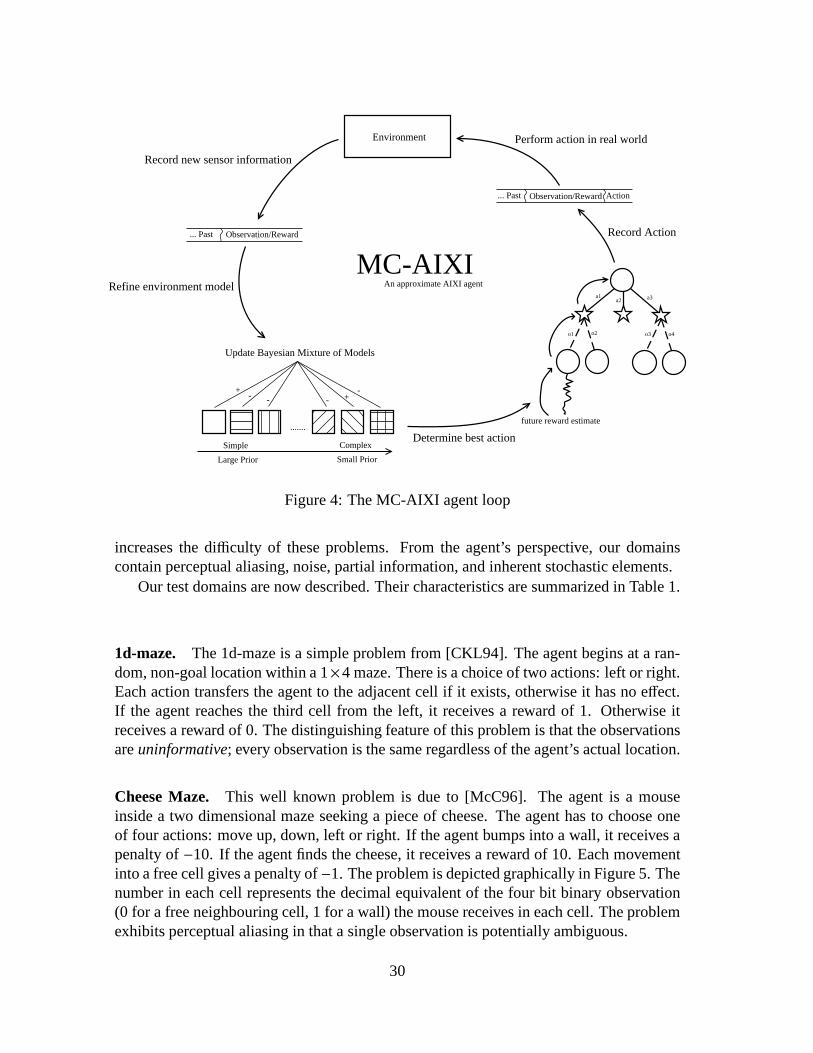
Top-level Algorithm. At each time step, MC-AIXI(fac-ctw) first invokes theρUCTroutine with a fixed horizon to estimate the value of each candidate action. An action isthen chosen according to some policy that balances exploration with exploitation, suchasǫ-Greedy or Softmax [SB98]. This action is communicated to the environment, whichresponds with an observation-reward pair. The agent then incorporates this informationinto Υ using the FAC-CTW algorithm and the cycle repeats. Figure 4 gives an overviewof the agent/environment interaction loop.
7 Experimental Results
We now measure our agent’s performance across a number of different domains. In par-ticular, we focused on learning and solving some well-knownbenchmark problems fromthe POMDP literature. Given the full POMDP model, computation of the optimal pol-icy for each of these POMDPs is not difficult. However, our requirement of having toboth learn a model of the environment, as well as find a good policy online,significantly
29
Environment
Update Bayesian Mixture of Models
a1a2 a3
o1 o2 o3 o4
future reward estimate
Record Action
Simple Complex
Large Prior Small Prior
+
.......
- - +-
-
Observation/Reward... Past
Determine best action
Action... Past Observation/Reward
Perform action in real world
Record new sensor information
Refine environment model
MC-AIXIAn approximate AIXI agent
Figure 4: The MC-AIXI agent loop
increases the difficulty of these problems. From the agent’s perspective, our domainscontain perceptual aliasing, noise, partial information,and inherent stochastic elements.
Our test domains are now described. Their characteristics are summarized in Table 1.
1d-maze. The 1d-maze is a simple problem from [CKL94]. The agent begins at a ran-dom, non-goal location within a 1×4 maze. There is a choice of two actions: left or right.Each action transfers the agent to the adjacent cell if it exists, otherwise it has no effect.If the agent reaches the third cell from the left, it receivesa reward of 1. Otherwise itreceives a reward of 0. The distinguishing feature of this problem is that the observationsareuninformative; every observation is the same regardless of the agent’s actual location.
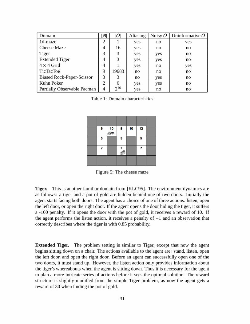
Cheese Maze. This well known problem is due to [McC96]. The agent is a mouseinside a two dimensional maze seeking a piece of cheese. The agent has to choose oneof four actions: move up, down, left or right. If the agent bumps into a wall, it receives apenalty of−10. If the agent finds the cheese, it receives a reward of 10. Each movementinto a free cell gives a penalty of−1. The problem is depicted graphically in Figure 5. Thenumber in each cell represents the decimal equivalent of thefour bit binary observation(0 for a free neighbouring cell, 1 for a wall) the mouse receives in each cell. The problemexhibits perceptual aliasing in that a single observation is potentially ambiguous.
30
Domain |A| |O| Aliasing NoisyO UninformativeO1d-maze 2 1 yes no yesCheese Maze 4 16 yes no noTiger 3 3 yes yes noExtended Tiger 4 3 yes yes no4 × 4 Grid 4 1 yes no yesTicTacToe 9 19683 no no noBiased Rock-Paper-Scissor 3 3 no yes noKuhn Poker 2 6 yes yes noPartially Observable Pacman 4 216 yes no no
Table 1: Domain characteristics
Figure 5: The cheese maze
Tiger. This is another familiar domain from [KLC95]. The environment dynamics areas follows: a tiger and a pot of gold are hidden behind one of two doors. Initially theagent starts facing both doors. The agent has a choice of one of three actions: listen, openthe left door, or open the right door. If the agent opens the door hiding the tiger, it suffersa -100 penalty. If it opens the door with the pot of gold, it receives a reward of 10. Ifthe agent performs the listen action, it receives a penalty of −1 and an observation thatcorrectly describes where the tiger is with 0.85 probability.
Extended Tiger. The problem setting is similar to Tiger, except that now the agentbegins sitting down on a chair. The actions available to the agent are: stand, listen, openthe left door, and open the right door. Before an agent can successfully open one of thetwo doors, it must stand up. However, the listen action only provides information aboutthe tiger’s whereabouts when the agent is sitting down. Thusit is necessary for the agentto plan a more intricate series of actions before it sees the optimal solution. The rewardstructure is slightly modified from the simple Tiger problem, as now the agent gets areward of 30 when finding the pot of gold.
31

4 × 4 Grid. The agent is restricted to a 4× 4 grid world. It can move either up, down,right or left. If the agent moves into the bottom right corner, it receives a reward of 1, andit is randomly teleported to one of the remaining 15 cells. Ifit moves into any cell otherthan the bottom right corner cell, it receives a reward of 0. If the agent attempts to moveinto a non-existent cell, it remains in the same location. Like the 1d-maze, this problemis also uninformative but on a much larger scale. Although this domain is simple, it doesrequire some subtlety on the part of the agent. The correct action depends on what theagent has tried before at previous time steps. For example, if the agent has repeatedlymoved right and not received a positive reward, then the chances of it receiving a positivereward by moving down are increased.
TicTacToe. In this domain, the agent plays repeated games of TicTacToe against anopponent who moves randomly. If the agent wins the game, it receives a reward of 2. Ifthere is a draw, the agent receives a reward of 1. A loss penalises the agent by−2. If theagent makes an illegal move, by moving on top of an already filled square, then it receivesa reward of−3. A legal move that does not end the game earns no reward.
Biased Rock-Paper-Scissors. This domain is taken from [FMVRW10]. The agent re-peatedly plays Rock-Paper-Scissor against an opponent that has a slight, predictable biasin its strategy. If the opponent has won a round by playing rock on the previous cycle,it will always play rock at the next cycle; otherwise it will pick an action uniformly atrandom. The agent’s observation is the most recently chosenaction of the opponent. Itreceives a reward of 1 for a win, 0 for a draw and−1 for a loss.
Kuhn Poker. Our next domain involves playing Kuhn Poker [Kuh50, HSHB05]againstan opponent playing a Nash strategy. Kuhn Poker is a simplified, zero-sum, two playerpoker variant that uses a deck of three cards: a King, Queen and Jack. Whilst consider-ably less sophisticated than popular poker variants such asTexas Hold’em, well-knownstrategic concepts such as bluffing and slow-playing remain characteristic of strong play.
In our setup, the agent acts second in a series of rounds. Two actions, pass or bet,are available to each player. A bet action requires the player to put an extra chip intoplay. At the beginning of each round, each player puts a chip into play. The opponentthen decides whether to pass or bet; betting will win the round if the agent subsequentlypasses, otherwise a showdown will occur. In a showdown, the player with the highestcard wins the round. If the opponent passes, the agent can either bet or pass; passingleads immediately to a showdown, whilst betting requires the opponent to either bet toforce a showdown, or to pass and let the agent win the round uncontested. The winner ofthe round gains a reward equal to the total chips in play, the loser receives a penalty equalto the number of chips they put into play this round. At the endof the round, all chips areremoved from play and another round begins.
Kuhn Poker has a known optimal solution. Against a first player playing a Nashstrategy, the second player can obtain at most an average reward of 1
18 per round.
32
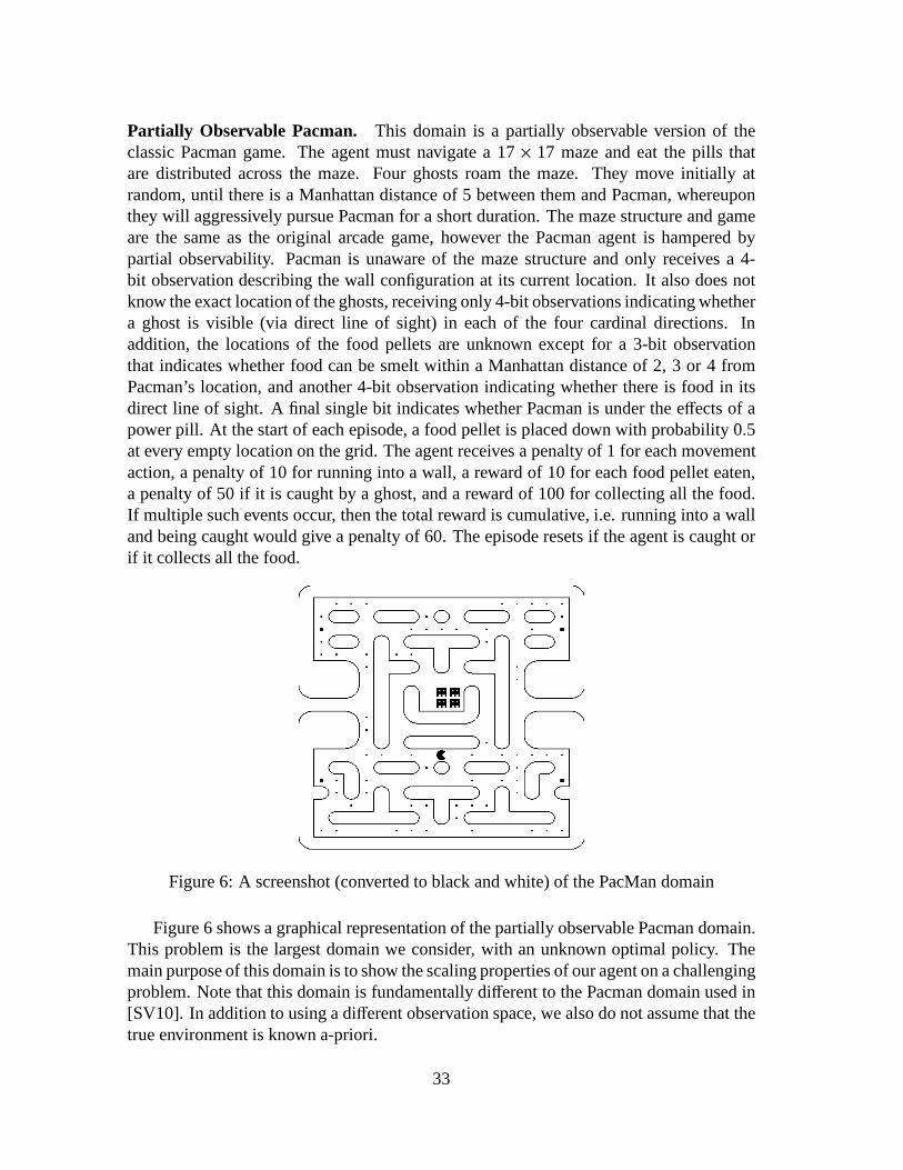
Partially Observable Pacman. This domain is a partially observable version of theclassic Pacman game. The agent must navigate a 17× 17 maze and eat the pills thatare distributed across the maze. Four ghosts roam the maze. They move initially atrandom, until there is a Manhattan distance of 5 between themand Pacman, whereuponthey will aggressively pursue Pacman for a short duration. The maze structure and gameare the same as the original arcade game, however the Pacman agent is hampered bypartial observability. Pacman is unaware of the maze structure and only receives a 4-bit observation describing the wall configuration at its current location. It also does notknow the exact location of the ghosts, receiving only 4-bit observations indicating whethera ghost is visible (via direct line of sight) in each of the four cardinal directions. Inaddition, the locations of the food pellets are unknown except for a 3-bit observationthat indicates whether food can be smelt within a Manhattan distance of 2, 3 or 4 fromPacman’s location, and another 4-bit observation indicating whether there is food in itsdirect line of sight. A final single bit indicates whether Pacman is under the effects of apower pill. At the start of each episode, a food pellet is placed down with probability 0.5at every empty location on the grid. The agent receives a penalty of 1 for each movementaction, a penalty of 10 for running into a wall, a reward of 10 for each food pellet eaten,a penalty of 50 if it is caught by a ghost, and a reward of 100 forcollecting all the food.If multiple such events occur, then the total reward is cumulative, i.e. running into a walland being caught would give a penalty of 60. The episode resets if the agent is caught orif it collects all the food.
Figure 6: A screenshot (converted to black and white) of the PacMan domain
Figure 6 shows a graphical representation of the partially observable Pacman domain.This problem is the largest domain we consider, with an unknown optimal policy. Themain purpose of this domain is to show the scaling propertiesof our agent on a challengingproblem. Note that this domain is fundamentally different to the Pacman domain used in[SV10]. In addition to using a different observation space, we also do not assume that thetrue environment is known a-priori.
33

Experimental Setup. We now evaluate the performance of the MC-AIXI(fac-ctw)agent. To help put our results into perspective, we implemented and directly comparedagainst two competing algorithms from the model-based general reinforcement learningliterature: U-Tree [McC96] and Active-LZ [FMVRW10]. The two algorithms are de-scribed on page 42 in Section 8. As FAC-CTW subsumes Action Conditional CTW, wedo not evaluate it in this paper; earlier results using Action Conditional CTW can be foundin [VNHS10]. The performance of the agent using FAC-CTW is noworse and in somecases slightly better than the previous results.
Each agent communicates with the environment over a binary channel. A cycle beginswith the agent sending an actiona to the environment, which then responds with a perceptx. This cycle is then repeated. A fixed number of bits are used toencode the action,observation and reward spaces for each domain. These are specified in Table 2. Noconstraint is placed on how the agent interprets the observation component; e.g., thiscould be done at either the bit or symbol level. The rewards are encoded naively, i.e. thebits corresponding to the reward are interpreted as unsigned integers. Negative rewardsare handled (without loss of generality) by offsetting all of the rewards so that they areguaranteed to be non-negative. These offsets are removed from the reported results.
Domain A bits O bits R bits1d-maze 1 1 1Cheese Maze 2 4 5Tiger 2 2 7Extended Tiger 2 3 84 × 4 Grid 2 1 1TicTacToe 4 18 3Biased Rock-Paper-Scissor 2 2 2Kuhn Poker 1 4 3Partially Observable Pacman 2 16 8
Table 2: Binary encoding of the domains
The process of gathering results for each of the three agentsis broken into two phases:model learning and model evaluation. The model learning phase involves running eachagent with an exploratory policy to build a model of the environment. This learnt model isthen evaluated at various points in time by running the agentwithout exploration for 5000cycles and reporting the average reward per cycle. More precisely, at timet the averagereward per cycle is defined as15000
∑t+5000i=t+1 r i, wherer i is the reward received at cycle
i. Having two separate phases reduces the influence of the agent’s earlier exploratoryactions on the reported performance. All of our experimentswere performed on a dualquad-core Intel 2.53Ghz Xeon with 24 gigabytes of memory.
Table 3 outlines the parameters used by MC-AIXI(fac-ctw) during the model learningphase. The context depth parameterD specifies the maximal number of recent bits used
34

Domain D m ǫ γ ρUCT Simulations1d-maze 32 10 0.9 0.99 500Cheese Maze 96 8 0.999 0.9999 500Tiger 96 5 0.99 0.9999 500Extended Tiger 96 4 0.99 0.99999 5004 × 4 Grid 96 12 0.9 0.9999 500TicTacToe 64 9 0.9999 0.999999 500Biased Rock-Paper-Scissor32 4 0.999 0.99999 500Kuhn Poker 42 2 0.99 0.9999 500Partial Observable Pacman96 4 0.9999 0.99999 500
Table 3: MC-AIXI(fac-ctw) model learning configuration
by FAC-CTW. TheρUCT search horizon is specified by the parameterm. LargerD andm increase the capabilities of our agent, at the expense of linearly increasing computa-tion time; our values represent an appropriate compromise between these two competingdimensions for each problem domain. Exploration during themodel learning phase iscontrolled by theǫ andγ parameters. At timet, MC-AIXI( fac-ctw) explores a randomaction with probabilityγtǫ. During the model evaluation phase, exploration is disabled,with results being recorded for varying amounts of experience and search effort.
The Active-LZ algorithm is fully specified in [FMVRW10]. It contains only two pa-rameters, a discount rate and a policy that balances betweenexploration and exploitation.During the model learning phase, a discount rate of 0.99 andǫ-Greedy exploration (withǫ = 0.95) were used. Smaller exploration values (such as 0.05, 0.2, 0.5) were tried, aswell as policies that decayedǫ over time, but these surprisingly gave slightly worse per-formance during testing. As a sanity check, we confirmed thatour implementation couldreproduce the experimental results reported in [FMVRW10].During the model evaluationphase, exploration is disabled.
The situation is somewhat more complicated for U-Tree, as itis more of a generalagent framework than a completely specified algorithm. Due to the absence of a publiclyavailable reference implementation, a number of implementation-specific decisions weremade. These included the choice of splitting criteria, how far back in time these criteriacould be applied, the frequency of fringe tests, the choice of p-value for the Kolmogorov-Smirnov test, the exploration/exploitation policy and the learning rate. The main designdecisions are listed below:
• A split could be made on any action, or on the status of any single bit of an obser-vation.
• The maximum number of steps backwards in time for which a utile distinction couldbe made was set to 5.
• The frequency of fringe tests was maximised given realisticresource constraints.Our choices allowed for 5× 10⁴ cycles of interaction to be completed on eachdomain within 2 days of training time.
35

Domain ǫ Test Fringe α
1d-maze 0.05 100 0.05Cheese Maze 0.2 100 0.05Tiger 0.1 100 0.05Extended Tiger 0.05 200 0.014 × 4 Grid 0.05 100 0.05TicTacToe 0.05 1000 0.01Biased Rock-Paper-Scissor0.05 100 0.05Kuhn Poker 0.05 200 0.05
Table 4: U-Tree model learning configuration
• Splits were tried in order from the most temporally recent tothe most temporallydistant.
• ǫ-Greedy exploration strategy was used, withǫ tuned separately for each domain.
• The learning rateα was tuned for each domain.
To help make the comparison as fair as possible, an effort was made to tune U-Tree’s pa-rameters for each domain. The final choices for the model learning phase are summarisedin Table 4. During the model evaluation phase, both exploration and testing of the fringeare disabled.
Source Code. The code for our U-Tree, Active-LZ and MC-AIXI(fac-ctw) implemen-tations can be found at:http://jveness.info/software/mcaixi_jair_2010.zip.
Results. Figure 7 presents our main set of results. Each graph shows the performanceof each agent as it accumulates more experience. The performance of MC-AIXI(fac-ctw)matches or exceeds U-Tree and Active-LZ on all of our test domains. Active-LZ steadilyimproved with more experience, however it learnt significantly more slowly than bothU-Tree and MC-AIXI(fac-ctw). U-Tree performed well in most domains, however theoverhead of testing for splits limited its ability to be run for long periods of time. Thisis the reason why some data points for U-Tree are missing fromthe graphs in Figure7. This highlights the advantage of algorithms that take constant time per cycle, suchas MC-AIXI(fac-ctw) and Active-LZ. Constant time isn’t enough however, especiallywhen large observation spaces are involved. Active-LZ works at the symbol level, withthe algorithm given by [FMVRW10] requiring an exhaustive enumeration of the perceptspace on each cycle. This is not possible in reasonable time for the larger TicTacToedomain, which is why no Active-LZ result is presented. This illustrates an importantadvantage of MC-AIXI(fac-ctw) and U-Tree, which have the ability to exploit structurewithin a single observation.
Figure 8 shows the performance of MC-AIXI(fac-ctw) as the number ofρUCT sim-ulations varies. The results for each domain were based on a model learnt from 5× 10⁴
cycles of experience, except in the case of TicTacToe where 5× 10⁵ cycles were used.
36
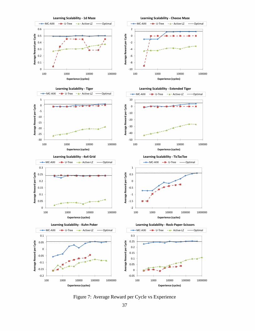
0
0.1
0.2
0.3
0.4
0.5
0.6
100 1000 10000 100000
Av
era
ge
Re
wa
rd p
er
Cy
cle
Experience (cycles)
Learning Scalability - 1d Maze
MC-AIXI U-Tree Active-LZ Optimal
-10
-8
-6
-4
-2
0
2
100 1000 10000 100000
Av
era
ge
Re
wa
rd p
er
Cy
cle
Experience (cycles)
Learning Scalability - Cheese Maze
MC-AIXI U-Tree Active-LZ Optimal
-30
-25
-20
-15
-10
-5
0
5
100 1000 10000 100000
Av
era
ge
Re
wa
rd p
er
Cy
cle
Experience (cycles)
Learning Scalability - Tiger
MC-AIXI U-Tree Active-LZ Optimal
-50
-40
-30
-20
-10
0
10
100 1000 10000 100000
Av
era
ge
Re
wa
rd p
er
Cy
cle
Experience (cycles)
Learning Scalability - Extended Tiger
MC-AIXI U-Tree Active-LZ Optimal
0
0.05
0.1
0.15
0.2
0.25
0.3
100 1000 10000 100000
Av
era
ge
Re
wa
rd p
er
Cy
cle
Experience (cycles)
Learning Scalability - 4x4 Grid
MC-AIXI U-Tree Active-LZ Optimal
-2
-1.5
-1
-0.5
0
0.5
1
100 1000 10000 100000 1000000
Av
era
ge
Re
wa
rd p
er
Cy
cle
Experience (cycles)
Learning Scalability - TicTacToe
MC-AIXI U-Tree Optimal
-0.2
-0.15
-0.1
-0.05
0
0.05
0.1
100 1000 10000 100000 1000000
Av
era
ge
Re
wa
rd p
er
Cy
cle
Experience (cycles)
Learning Scalability - Kuhn Poker
MC-AIXI U-Tree Active-LZ Optimal
-0.05
0
0.05
0.1
0.15
0.2
0.25
0.3
100 1000 10000 100000 1000000
Av
era
ge
Re
wa
rd p
er
Cy
cle
Experience (cycles)
Learning Scalability - Rock-Paper-Scissors
MC-AIXI U-Tree Active-LZ Optimal
Figure 7: Average Reward per Cycle vs Experience
37
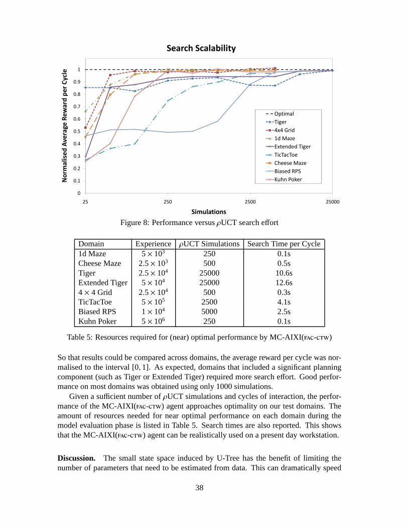
0
0.1
0.2
0.3
0.4
0.5
0.6
0.7
0.8
0.9
1
25 250 2500 25000
No
rma
lise
d A
ve
rag
e R
ew
ard
pe
r C
ycl
e
Simulations
Search Scalability
Optimal
Tiger
4x4 Grid
1d Maze
Extended Tiger
TicTacToe
Cheese Maze
Biased RPS
Kuhn Poker
Figure 8: Performance versusρUCT search effort
Domain Experience ρUCT Simulations Search Time per Cycle1d Maze 5× 10³ 250 0.1sCheese Maze 2.5× 10³ 500 0.5sTiger 2.5× 10⁴ 25000 10.6sExtended Tiger 5× 10⁴ 25000 12.6s4 × 4 Grid 2.5× 10⁴ 500 0.3sTicTacToe 5× 10⁵ 2500 4.1sBiased RPS 1× 10⁴ 5000 2.5sKuhn Poker 5× 10⁶ 250 0.1s
Table 5: Resources required for (near) optimal performanceby MC-AIXI( fac-ctw)
So that results could be compared across domains, the average reward per cycle was nor-malised to the interval [0, 1]. As expected, domains that included a significant planningcomponent (such as Tiger or Extended Tiger) required more search effort. Good perfor-mance on most domains was obtained using only 1000 simulations.
Given a sufficient number ofρUCT simulations and cycles of interaction, the perfor-mance of the MC-AIXI(fac-ctw) agent approaches optimality on our test domains. Theamount of resources needed for near optimal performance on each domain during themodel evaluation phase is listed in Table 5. Search times arealso reported. This showsthat the MC-AIXI(fac-ctw) agent can be realistically used on a present day workstation.
Discussion. The small state space induced by U-Tree has the benefit of limiting thenumber of parameters that need to be estimated from data. This can dramatically speed
38

up the model-learning process. In contrast, both Active-LZand our approach require anumber of parameters proportional to the number of distinctcontexts. This is one of thereasons why Active-LZ exhibits slow convergence in practice. This problem is much lesspronounced in our approach for two reasons. First, the Ockham prior in CTW ensuresthat future predictions are dominated by PST structures that have seen enough data to betrustworthy. Secondly, value function estimation is decoupled from the process of contextestimation. Thus it is reasonable to expectρUCT to make good local decisions providedFAC-CTW can predict well. The downside however is that our approach requires searchfor action selection. AlthoughρUCT is an anytime algorithm, in practice more com-putation (at least on small domains) is required per cycle compared to approaches likeActive-LZ and U-Tree that act greedily with respect to an estimated global value func-tion.
The U-Tree algorithm is well motivated, but unlike Active-LZ and our approach, itlacks theoretical performance guarantees. It is possible for U-Tree to prematurely con-verge to a locally optimal state representation from which the heuristic splitting criterioncan never recover. Furthermore, the splitting heuristic contains a number of configurationoptions that can dramatically influence its performance [McC96]. This parameter sensi-tivity somewhat limits the algorithm’s applicability to the general reinforcement learningproblem. Still, our results suggest that further investigation of frameworks motivatedalong the same lines as U-Tree is warranted.
Comparison to 1-ply Rollout Planning. We now investigate the performance ofρUCTin comparison to an adaptation of the well-known 1-ply rollout-based planning techniqueof [BC99]. In our setting, this works as follows: given a history h, an estimateV(ha) isconstructed for each actiona ∈ A, by averaging the returns of many lengthmsimulationsinitiated fromha. The first action of each simulation is sampled uniformly at randomfrom A, whilst the remaining actions are selected according to some heuristic rolloutpolicy. Once a sufficient number of simulations have been completed, the actionwith thehighest estimated value is selected. UnlikeρUCT, this procedure doesn’t build a tree,nor is it guaranteed to converge to the depthm expectimax solution. In practice however,especially in noisy and highly stochastic domains, rollout-based planning can significantlyimprove the performance of an existing heuristic rollout policy [BC99].
Table 6 shows how the performance (given by average reward per cycle) differs whenρUCT is replaced by the 1-ply rollout planner. The amount of experience collected bythe agent, as well as the total number of rollout simulations, is the same as in Table 5.Both ρUCT and the 1-ply planner use the same search horizon, heuristic rollout policy(each action is chosen uniformly at random) and total numberof simulations for eachdecision. This is reasonable, since althoughρUCT has a slightly higher overhead com-pared to the 1-ply rollout planner, this difference is negligible when taking into accountthe cost of simulating future trajectories using FAC-CTW. Also, similar to previous ex-periments, 5000 cycles of greedy action selection were usedto evaluate the performanceof the FAC-CTW+ 1-ply rollout planning combination.
Importantly,ρUCT never gives worse performance than the 1-ply rollout planner, and
39

Domain MC-AIXI( fac-ctw) FAC-CTW+ 1-ply MC1d Maze 0.50 0.50Cheese Maze 1.28 1.25Tiger 1.12 1.11Extended Tiger 3.97 -0.974x4 Grid 0.24 0.24TicTacToe 0.60 0.59Biased RPS 0.25 0.20Kuhn Poker 0.06 0.06
Table 6: Average reward per cycle:ρUCT versus 1-ply rollout planning
on some domains (shown in bold) performs better. TheρUCT algorithm provides a wayof performing multi-step planning whilst retaining the considerable computational advan-tages of rollout based methods. In particular,ρUCT will be able to construct deep plansin regions of the search space where most of the probability mass is concentrated on asmall set of the possible percepts. When such structure exists,ρUCT will automaticallyexploit it. In the worst case where the environment is highlynoisy or stochastic, the per-formance will be similar to that of rollout based planning. Interestingly, on many domainsthe empirical performance of 1-ply rollout planning matched that ofρUCT. We believethis to be a byproduct of our modest set of test domains, wheremulti-step planning is lessimportant than learning an accurate model of the environment.
Performance on a Challenging Domain. The performance of MC-AIXI(fac-ctw) wasalso evaluated on the challenging Partially Observable Pacman domain. This is an enor-mous problem. Even if the true environment were known, planning would still be difficultdue to the 1060 distinct underlying states.
We first evaluated the performance of MC-AIXI(fac-ctw) online. A discountedǫ-Greedy policy, which chose a random action at timet with probabilityǫγt was used. Theseparameters were instantiated withǫ := 0.9999 andγ := 0.99999. When not exploring,each action was determined byρUCT using 500 simulations. Figure 10 shows both theaverage reward per cycle and the average reward across the most recent 5000 cycles.
The performance of this learnt model was then evaluated by performing 5000 steps ofgreedy action selection, at various time points, whilst varying the number of simulationsused byρUCT. Figure 9 shows obtained results. The agent’s performance scales withboth the number of cycles of interaction and the amount of search effort. The results inFigure 9 using 500 simulations are higher than in Figure 10 since the performance is nolonger affected by the exploration policy or earlier behavior based onan inferior learntmodel.
Visual inspection1 of Pacman shows that the agent, whilst not playing perfectly, hasalready learnt a number of important concepts. It knows not to run into walls. It knows
1Seehttp://jveness.info/publications/pacman_jair_2010.wmv for a graphical demonstration
40
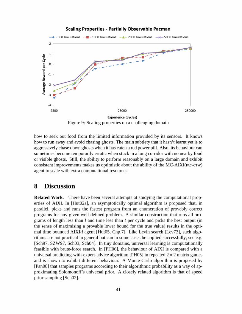
-4
-3
-2
-1
0
1
2
2500 25000 250000
Av
era
ge
Re
wa
rd p
er
Cy
cle
Experience (cycles)
Scaling Properties - Partially Observable Pacman
500 simulations 1000 simulations 2000 simulations 5000 simulations
Figure 9: Scaling properties on a challenging domain
how to seek out food from the limited information provided byits sensors. It knowshow to run away and avoid chasing ghosts. The main subtlety that it hasn’t learnt yet is toaggressively chase down ghosts when it has eaten a red power pill. Also, its behaviour cansometimes become temporarily erratic when stuck in a long corridor with no nearby foodor visible ghosts. Still, the ability to perform reasonablyon a large domain and exhibitconsistent improvements makes us optimistic about the ability of the MC-AIXI(fac-ctw)agent to scale with extra computational resources.
8 Discussion
Related Work. There have been several attempts at studying the computational prop-erties of AIXI. In [Hut02a], an asymptotically optimal algorithm is proposed that, inparallel, picks and runs the fastest program from an enumeration of provably correctprograms for any given well-defined problem. A similar construction that runs all pro-grams of length less thanl and time less thant per cycle and picks the best output (inthe sense of maximising a provable lower bound for the true value) results in the opti-mal time bounded AIXItl agent [Hut05, Chp.7]. Like Levin search [Lev73], such algo-rithms are not practical in general but can in some cases be applied successfully; see e.g.[Sch97, SZW97, Sch03, Sch04]. In tiny domains, universal learning is computationallyfeasible with brute-force search. In [PH06], the behaviourof AIXI is compared with auniversal predicting-with-expert-advice algorithm [PH05] in repeated 2× 2 matrix gamesand is shown to exhibit different behaviour. A Monte-Carlo algorithm is proposed by[Pan08] that samples programs according to their algorithmic probability as a way of ap-proximating Solomonoff’s universal prior. A closely related algorithm is that of speedprior sampling [Sch02].
41
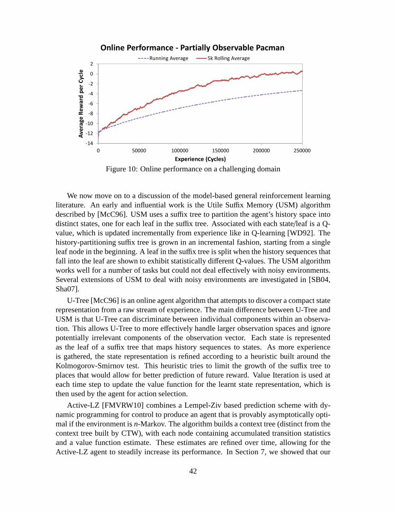
-14
-12
-10
-8
-6
-4
-2
0
2
0 50000 100000 150000 200000 250000
Experience (Cycles)
Online Performance - Partially Observable Pacman
Running Average 5k Rolling Average
Figure 10: Online performance on a challenging domain
We now move on to a discussion of the model-based general reinforcement learningliterature. An early and influential work is the Utile Suffix Memory (USM) algorithmdescribed by [McC96]. USM uses a suffix tree to partition the agent’s history space intodistinct states, one for each leaf in the suffix tree. Associated with each state/leaf is a Q-value, which is updated incrementally from experience likein Q-learning [WD92]. Thehistory-partitioning suffix tree is grown in an incremental fashion, starting from a singleleaf node in the beginning. A leaf in the suffix tree is split when the history sequences thatfall into the leaf are shown to exhibit statistically different Q-values. The USM algorithmworks well for a number of tasks but could not deal effectively with noisy environments.Several extensions of USM to deal with noisy environments are investigated in [SB04,Sha07].
U-Tree [McC96] is an online agent algorithm that attempts todiscover a compact staterepresentation from a raw stream of experience. The main difference between U-Tree andUSM is that U-Tree can discriminate between individual components within an observa-tion. This allows U-Tree to more effectively handle larger observation spaces and ignorepotentially irrelevant components of the observation vector. Each state is representedas the leaf of a suffix tree that maps history sequences to states. As more experienceis gathered, the state representation is refined according to a heuristic built around theKolmogorov-Smirnov test. This heuristic tries to limit thegrowth of the suffix tree toplaces that would allow for better prediction of future reward. Value Iteration is used ateach time step to update the value function for the learnt state representation, which isthen used by the agent for action selection.
Active-LZ [FMVRW10] combines a Lempel-Ziv based prediction scheme with dy-namic programming for control to produce an agent that is provably asymptotically opti-mal if the environment isn-Markov. The algorithm builds a context tree (distinct fromthecontext tree built by CTW), with each node containing accumulated transition statisticsand a value function estimate. These estimates are refined over time, allowing for theActive-LZ agent to steadily increase its performance. In Section 7, we showed that our
42
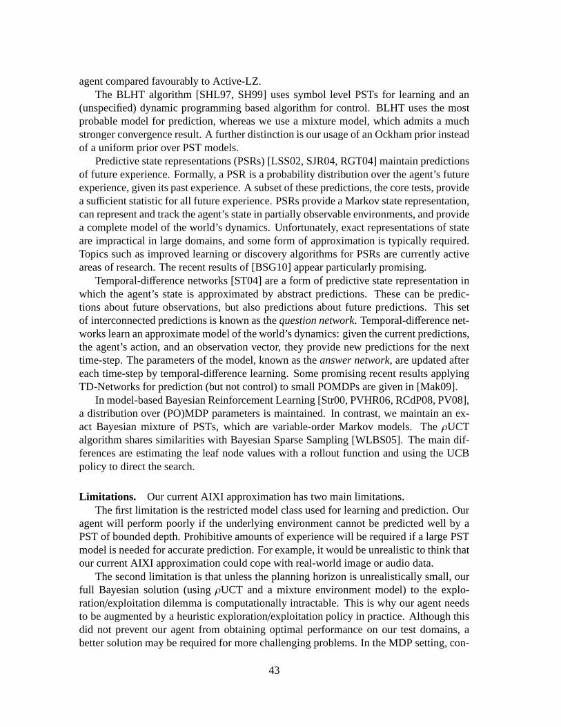
agent compared favourably to Active-LZ.The BLHT algorithm [SHL97, SH99] uses symbol level PSTs for learning and an
(unspecified) dynamic programming based algorithm for control. BLHT uses the mostprobable model for prediction, whereas we use a mixture model, which admits a muchstronger convergence result. A further distinction is our usage of an Ockham prior insteadof a uniform prior over PST models.
Predictive state representations (PSRs) [LSS02, SJR04, RGT04] maintain predictionsof future experience. Formally, a PSR is a probability distribution over the agent’s futureexperience, given its past experience. A subset of these predictions, the core tests, providea sufficient statistic for all future experience. PSRs provide a Markov state representation,can represent and track the agent’s state in partially observable environments, and providea complete model of the world’s dynamics. Unfortunately, exact representations of stateare impractical in large domains, and some form of approximation is typically required.Topics such as improved learning or discovery algorithms for PSRs are currently activeareas of research. The recent results of [BSG10] appear particularly promising.
Temporal-difference networks [ST04] are a form of predictive state representation inwhich the agent’s state is approximated by abstract predictions. These can be predic-tions about future observations, but also predictions about future predictions. This setof interconnected predictions is known as thequestion network. Temporal-difference net-works learn an approximate model of the world’s dynamics: given the current predictions,the agent’s action, and an observation vector, they providenew predictions for the nexttime-step. The parameters of the model, known as theanswer network, are updated aftereach time-step by temporal-difference learning. Some promising recent results applyingTD-Networks for prediction (but not control) to small POMDPs are given in [Mak09].
In model-based Bayesian Reinforcement Learning [Str00, PVHR06, RCdP08, PV08],a distribution over (PO)MDP parameters is maintained. In contrast, we maintain an ex-act Bayesian mixture of PSTs, which are variable-order Markov models. TheρUCTalgorithm shares similarities with Bayesian Sparse Sampling [WLBS05]. The main dif-ferences are estimating the leaf node values with a rollout function and using the UCBpolicy to direct the search.
Limitations. Our current AIXI approximation has two main limitations.The first limitation is the restricted model class used for learning and prediction. Our
agent will perform poorly if the underlying environment cannot be predicted well by aPST of bounded depth. Prohibitive amounts of experience will be required if a large PSTmodel is needed for accurate prediction. For example, it would be unrealistic to think thatour current AIXI approximation could cope with real-world image or audio data.
The second limitation is that unless the planning horizon isunrealistically small, ourfull Bayesian solution (usingρUCT and a mixture environment model) to the explo-ration/exploitation dilemma is computationally intractable. This is why our agent needsto be augmented by a heuristic exploration/exploitation policy in practice. Although thisdid not prevent our agent from obtaining optimal performance on our test domains, abetter solution may be required for more challenging problems. In the MDP setting, con-
43

siderable progress has been made towards resolving the exploration/exploitation issue.In particular, powerful PAC-MDP approaches exist for both model-based and model-freereinforcement learning agents [BT03, SLW+06, SLL09]. It remains to be seen whethersimilar such principled approaches exist for history-based Bayesian agents.
9 Future Scalability
We now list some ideas that make us optimistic about the future scalability of our ap-proach.
Online Learning of Rollout Policies for ρUCT. An important parameter toρUCTis the choice of rollout policy. In MCTS methods for ComputerGo, it is well knownthat search performance can be improved by using knowledge-based rollout policies[GWMT06]. In the general agent setting, it would thus be desirable to gain some ofthe benefits of expert design through online learning.
We have conducted some preliminary experiments in this area. A CTW-based methodwas used to predict the high-level actions chosen online byρUCT. This learnt distributionreplaced our previous uniformly random rollout policy. Figure 11 shows the results ofusing this learnt rollout policy on the cheese maze. The other domains we tested exhibitedsimilar behaviour. Although more work remains, it is clear that even our current simplelearning scheme can significantly improve the performance of ρUCT.
Although our first attempts have been promising, a more thorough investigation isrequired. It is likely that rollout policy learning methodsfor adversarial games, such as[ST09], can be adapted to our setting. It would also be interesting to try to apply someform of search bootstrapping [VSUB09] online. In addition,one could also look at waysto modify the UCB policy used inρUCT to automatically take advantage of learnt rolloutknowledge, similar to the heuristic techniques used in computer Go [GS07].
Combining Mixture Environment Models. A key property of mixture environmentmodels is that they can becomposed. Given two mixture environment modelsξ1 andξ2,over model classesM1 andM2 respectively, it is easy to show that the convex combina-tion
ξ(x1:n | a1:n) := αξ1(x1:n | a1:n) + (1− α)ξ2(x1:n | a1:n)
is a mixture environment model over the union ofM1 andM2. Thus there is a principledway for expanding the general predictive power of agents that use our kind of direct AIXIapproximation.
Richer Notions of Context for FAC-CTW. Instead of using the most recentD bitsof the current historyh, the FAC-CTW algorithm can be generalised to use a set ofDboolean functions onh to define the current context. We now formalise this notion, andgive some examples of how this might help in agent applications.
44
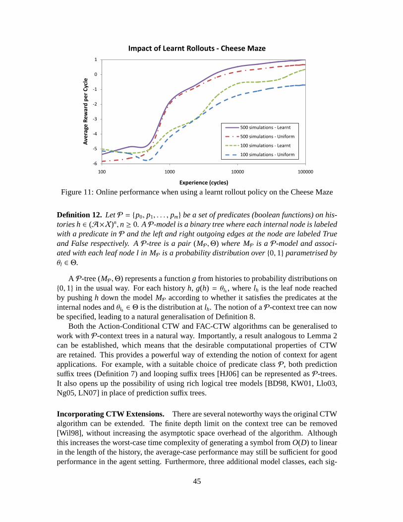
-6
-5
-4
-3
-2
-1
0
1
100 1000 10000 100000
Av
era
ge
Re
wa
rd p
er
Cy
cle
Experience (cycles)
Impact of Learnt Rollouts - Cheese Maze
500 simulations - Learnt
500 simulations - Uniform
100 simulations - Learnt
100 simulations - Uniform
Figure 11: Online performance when using a learnt rollout policy on the Cheese Maze
Definition 12. LetP = {p0, p1, . . . , pm} be a set of predicates (boolean functions) on his-tories h∈ (A×X)n, n ≥ 0. AP-model is a binary tree where each internal node is labeledwith a predicate inP and the left and right outgoing edges at the node are labeled Trueand False respectively. AP-tree is a pair(MP,Θ) where MP is aP-model and associ-ated with each leaf node l in MP is a probability distribution over{0, 1} parametrised byθl ∈ Θ.
A P-tree (MP,Θ) represents a functiong from histories to probability distributions on{0, 1} in the usual way. For each historyh, g(h) = θlh, wherelh is the leaf node reachedby pushingh down the modelMP according to whether it satisfies the predicates at theinternal nodes andθlh ∈ Θ is the distribution atlh. The notion of aP-context tree can nowbe specified, leading to a natural generalisation of Definition 8.
Both the Action-Conditional CTW and FAC-CTW algorithms canbe generalised towork with P-context trees in a natural way. Importantly, a result analogous to Lemma 2can be established, which means that the desirable computational properties of CTWare retained. This provides a powerful way of extending the notion of context for agentapplications. For example, with a suitable choice of predicate classP, both predictionsuffix trees (Definition 7) and looping suffix trees [HJ06] can be represented asP-trees.It also opens up the possibility of using rich logical tree models [BD98, KW01, Llo03,Ng05, LN07] in place of prediction suffix trees.
Incorporating CTW Extensions. There are several noteworthy ways the original CTWalgorithm can be extended. The finite depth limit on the context tree can be removed[Wil98], without increasing the asymptotic space overheadof the algorithm. Althoughthis increases the worst-case time complexity of generating a symbol fromO(D) to linearin the length of the history, the average-case performance may still be sufficient for goodperformance in the agent setting. Furthermore, three additional model classes, each sig-
45
nificantly larger than the one used by CTW, are presented in [WST96]. These could bemade action conditional along the same lines as our FAC-CTW derivation. Unfortunately,online prediction with these more general classes is now exponential in the context depthD. Investigating whether these ideas can be applied in a more restricted sense would bean interesting direction for future research.
Parallelization of ρUCT. The performance of our agent is dependent on the amountof thinking time allowed at each time step. An important property of ρUCT is that it isnaturally parallel. We have completed a prototype parallelimplementation ofρUCT withpromising scaling results using between 4 and 8 processing cores. We are confident thatfurther improvements to our implementation will allow us tosolve problems where ouragent’s planning ability is the main limitation.
Predicting at Multiple Levels of Abstraction. The FAC-CTW algorithm reduces thetask of predicting a single percept to the prediction of its binary representation. Whilstthis is reasonable for a first attempt at AIXI approximation,it’s worth emphasising thatsubsequent attempts need not work exclusively at such a low level.
For example, recall that the FAC-CTW algorithm was obtainedby chaining togetherlX action-conditional binary predictors. It would be straightforward to apply a similartechnique to chain together multiplek-bit action-conditional predictors, fork > 1. Thesek bits could be interpreted in many ways: e.g. integers, floating point numbers, ASCIIcharacters or even pixels. This observation, along with theconvenient property that mix-ture environment models can be composed, opens up the possibility of constructing moresophisticated,hierarchicalmixture environment models.
10 Conclusion
This paper presents the first computationally feasible general reinforcement learning agentthatdirectlyandscalablyapproximates the AIXI ideal. Although well established theoret-ically, it has previously been unclear whether the AIXI theory could inspire the design ofpractical agent algorithms. Our work answers this questionin the affirmative: empirically,our approximation achieves strong performance and theoretically, we can characterise therange of environments in which our agent is expected to perform well.
To develop our approximation, we introduced two new algorithms:ρUCT, a Monte-Carlo expectimax approximation technique that can be used with any online Bayesianapproach to the general reinforcement learning problem andFAC-CTW, a generalisationof the powerful CTW algorithm to the agent setting. In addition, we highlighted a numberof interesting research directions that could improve the performance of our current agent;in particular, model class expansion and the online learning of heuristic rollout policiesfor ρUCT.
We hope that this work generates further interest from the broader artificial intelli-gence community in both the AIXI theory and general reinforcement learning agents.
46
Acknowledgments. The authors thank Alan Blair, Thomas Degris-Dard, Evan Green-smith, Bernhard Hengst, Ramana Kumar, John Lloyd, Hassan Mahmud, Malcolm Ryan,Scott Sanner, Rich Sutton, Eric Wiewiora, Frans Willems andthe anonymous review-ers for helpful comments and feedback. This work received support from the AustralianResearch Council under grant DP0988049. NICTA is funded by the Australian Govern-ment’s Department of Communications, Information Technology, and the Arts and theAustralian Research Council through Backing Australia’s Ability and the ICT ResearchCentre of Excellence programs.
References
[Aue02] Peter Auer. Using confidence bounds for exploitation-exploration trade-offs. Journalof Machine Learning Research, 3:397–422, 2002.
[BC99] Dimitri P. Bertsekas and David A. Castanon. Rollout algorithms for stochastic schedul-ing problems.Journal of Heuristics, 5(1):89–108, 1999.
[BD98] Hendrik Blockeel and Luc De Raedt. Top-down induction of first-order logical deci-sion trees.Artificial Intelligence, 101(1-2):285–297, 1998.
[BEYY04] Ron Begleiter, Ran El-Yaniv, and Golan Yona. On prediction using variable orderMarkov models.Journal of Artificial Intelligence Research, 22:385–421, 2004.
[BSG10] Byron Boots, Sajid M. Siddiqi, and Geoffrey J. Gordon. Closing the learning-planningloop with predictive state representations. InProceedings of the 9th International Con-ference on Autonomous Agents and Multiagent Systems: volume 1 - Volume 1, AAMAS’10, pages 1369–1370, Richland, SC, 2010. International Foundation for AutonomousAgents and Multiagent Systems.
[BT03] Ronen I. Brafman and Moshe Tennenholtz. R-max - a general polynomial time algo-rithm for near-optimal reinforcement learning.Journal of Machine Learning Research,3:213–231, 2003.
[CKL94] Anthony R. Cassandra, Leslie Pack Kaelbling, and Michael L. Littman. Acting opti-mally in partially observable stochastic domains. InAAAI, pages 1023–1028, 1994.
[CT91] Thomas M. Cover and Joy A. Thomas.Elements of information theory. Wiley-Interscience, New York, NY, USA, 1991.
[CWH08] Guillaume M. Chaslot, Mark H. Winands, and H. Jaap Herik. Parallel monte-carlo treesearch. InProceedings of the 6th International Conference on Computers and Games,pages 60–71, Berlin, Heidelberg, 2008. Springer-Verlag.
[CWU+08] G.M.J-B. Chaslot, M.H.M. Winands, J.W.H.M. Uiterwijk,H.J. van den Herik, andB. Bouzy. Progressive strategies for Monte-Carlo Tree Search. New Mathematics andNatural Computation, 4(3):343–357, 2008.
[FB08] Hilmar Finnsson and Yngvi Bjornsson. Simulation-based approach to general gameplaying. InAAAI, pages 259–264, 2008.
[FMVRW10] V.F. Farias, C.C. Moallemi, B. Van Roy, and T. Weissman. Universal reinforcementlearning.Information Theory, IEEE Transactions on, 56(5):2441 –2454, may 2010.
47

[GS07] S. Gelly and D. Silver. Combining online and offline learning in UCT. InProceedingsof the 17th International Conference on Machine Learning, pages 273–280, 2007.
[GW06] Sylvain Gelly and Yizao Wang. Exploration exploitation in Go: UCT for Monte-CarloGo. InNIPS Workshop on On-line trading of Exploration and Exploitation, 2006.
[GWMT06] Sylvain Gelly, Yizao Wang, Remi Munos, and Olivier Teytaud. Modification of UCTwith patterns in Monte-Carlo Go. Technical Report 6062, INRIA, France, November2006.
[HJ06] Michael P. Holmes and Charles Lee Isbell Jr. Looping suffix tree-based inference ofpartially observable hidden state. InICML, pages 409–416, 2006.
[HSHB05] Bret Hoehn, Finnegan Southey, Robert C. Holte, andValeriy Bulitko. Effective short-term opponent exploitation in simplified poker. InAAAI, pages 783–788, 2005.
[Hut02a] Marcus Hutter. The fastest and shortest algorithmfor all well-defined problems.Inter-national Journal of Foundations of Computer Science., 13(3):431–443, 2002.
[Hut02b] Marcus Hutter. Self-optimizing and Pareto-optimal policies in general environmentsbased on Bayes-mixtures. InProceedings of the 15th Annual Conference on Com-putational Learning Theory (COLT 2002), Lecture Notes in Artificial Intelligence.Springer, 2002.
[Hut05] Marcus Hutter.Universal Artificial Intelligence: Sequential Decisions Based on Algo-rithmic Probability. Springer, 2005.
[Hut07] Marcus Hutter. Universal algorithmic intelligence: A mathematical top→down ap-proach. InArtificial General Intelligence, pages 227–290. Springer, Berlin, 2007.
[KLC95] Leslie Pack Kaelbling, Michael L. Littman, and Anthony R. Cassandra. Planning andacting in partially observable stochastic domains.Artificial Intelligence, 101:99–134,1995.
[KS06] Levente Kocsis and Csaba Szepesvari. Bandit based Monte-Carlo planning. InECML,pages 282–293, 2006.
[KT81] R.E. Krichevsky and V.K. Trofimov. The performance ofuniversal coding. IEEETransactions on Information Theory, IT-27:199–207, 1981.
[Kuh50] H. W. Kuhn. A simplified two-person poker. InContributions to the Theory of Games,pages 97–103, 1950.
[KW01] Stefan Kramer and Gerhard Widmer. Inducing classification and regression trees infirst order logic. In Saso Dzeroski and Nada Lavrac, editors, Relational Data Mining,chapter 6. Springer, 2001.
[Leg08] Shane Legg.Machine Super Intelligence. PhD thesis, Department of Informatics,University of Lugano, 2008.
[Lev73] Leonid A. Levin. Universal sequential search problems. Problems of InformationTransmission, 9:265–266, 1973.
[LH04] S. Legg and M. Hutter. Ergodic MDPs admit self-optimising policies. Technical ReportIDSIA-21-04, Dalle Molle Institute for Artificial Intelligence (IDSIA), 2004.
[Llo03] John W. Lloyd. Logic for Learning: Learning Comprehensible Theories fromStruc-tured Data. Springer, 2003.
48

[LN07] John W. Lloyd and Kee Siong Ng. Learning modal theories. In Proceedings of the16th International Conference on Inductive Logic Programming, LNAI 4455, pages320–334, 2007.
[LSS02] Michael Littman, Richard Sutton, and Satinder Singh. Predictive representations ofstate. InNIPS, pages 1555–1561, 2002.
[LV08] Ming Li and Paul Vitanyi. An Introduction to Kolmogorov Complexity and Its Appli-cations. Springer, third edition, 2008.
[Mak09] Takaki Makino. Proto-predictive representation of states with simple recurrenttemporal-difference networks. InICML, pages 697–704, 2009.
[McC96] Andrew Kachites McCallum.Reinforcement Learning with Selective Perception andHidden State. PhD thesis, University of Rochester, 1996.
[Ng05] Kee Siong Ng.Learning Comprehensible Theories from Structured Data. PhD thesis,The Australian National University, 2005.
[Pan08] Sergey Pankov. A computational approximation to the AIXI model. In AGI, pages256–267, 2008.
[PH05] Jan Poland and Marcus Hutter. Defensive universal learning with experts. InProc.16th International Conf. on Algorithmic Learning Theory, volume LNAI 3734, pages356–370. Springer, 2005.
[PH06] Jan Poland and Marcus Hutter. Universal learning of repeated matrix games. TechnicalReport 18-05, IDSIA, 2006.
[PV08] Pascal Poupart and Nikos Vlassis. Model-based bayesian reinforcement learning inpartially observable domains. InISAIM, 2008.
[PVHR06] Pascal Poupart, Nikos Vlassis, Jesse Hoey, and Kevin Regan. An analytic solutionto discrete bayesian reinforcement learning. InICML ’06: Proceedings of the 23rdinternational conference on Machine learning, pages 697–704, New York, NY, USA,2006. ACM.
[RCdP08] Stephane Ross, Brahim Chaib-draa, and Joelle Pineau. Bayes-adaptive POMDPs. InJ.C. Platt, D. Koller, Y. Singer, and S. Roweis, editors,Advances in Neural InformationProcessing Systems 20, pages 1225–1232. MIT Press, Cambridge, MA, 2008.
[RGT04] Matthew Rosencrantz, Geoffrey Gordon, and Sebastian Thrun. Learning low dimen-sional predictive representations. InProceedings of the twenty-first International Con-ference on Machine Learning, page 88, New York, NY, USA, 2004. ACM.
[Ris83] Jorma Rissanen. A universal data compression system. IEEE Transactions on Infor-mation Theory, 29(5):656–663, 1983.
[RST96] D. Ron, Y. Singer, and N. Tishby. The power of amnesia: Learning probabilisticautomata with variable memory length.Machine Learning, 25(2):117–150, 1996.
[SB98] Richard S. Sutton and Andrew G. Barto.Reinforcement Learning: An Introduction.MIT Press, 1998.
[SB04] Guy Shani and Ronen Brafman. Resolving perceptual aliasing in the presence of noisysensors. InNIPS, 2004.
49
[Sch97] Jurgen Schmidhuber. Discovering neural nets withlow Kolmogorov complexity andhigh generalization capability.Neural Networks, 10(5):857–873, 1997.
[Sch02] Jurgen Schmidhuber. The speed prior: A new simplicity measure yielding near-optimalcomputable predictions. InProc. 15th Annual Conf. on Computational Learning The-ory, pages 216–228, 2002.
[Sch03] Jurgen Schmidhuber. Bias-optimal incremental problem solving. InAdvances in Neu-ral Information Processing Systems 15, pages 1571–1578. MIT Press, 2003.
[Sch04] Jurgen Schmidhuber. Optimal ordered problem solver. Machine Learning, 54:211–254, 2004.
[SH99] Nobuo Suematsu and Akira Hayashi. A reinforcement learning algorithm in partiallyobservable environments using short-term memory. InNIPS, pages 1059–1065, 1999.
[Sha07] Guy Shani.Learning and Solving Partially Observable Markov DecisionProcesses.PhD thesis, Ben-Gurion University of the Negev, 2007.
[SHL97] Nobuo Suematsu, Akira Hayashi, and Shigang Li. A Bayesian approach to modellearning in non-Markovian environment. InICML, pages 349–357, 1997.
[SJR04] Satinder Singh, Michael James, and Matthew Rudary.Predictive state representations:A new theory for modeling dynamical systems. InUAI, pages 512–519, 2004.
[SLL09] Alexander L. Strehl, Lihong Li, and Michael L. Littman. Reinforcement learning infinite MDPs: PAC analysis.Journal of Machine Learning Research, 10:2413–2444,2009.
[SLW+06] Alexander L. Strehl, Lihong Li, Eric Wiewiora, John Langford, and Michael L.Littman. PAC model-free reinforcement learning. InICML ’06: Proceedings of the23rd international conference on Machine learning, pages 881–888, New York, NY,USA, 2006. ACM.
[Sol64] Ray J. Solomonoff. A formal theory of inductive inference: Parts 1 and 2.Informationand Control, 7:1–22 and 224–254, 1964.
[ST04] Richard S. Sutton and Brian Tanner. Temporal-difference networks. InNIPS, 2004.
[ST09] David Silver and Gerald Tesauro. Monte-carlo simulation balancing. InICML ’09:Proceedings of the 26th Annual International Conference onMachine Learning, pages945–952, New York, NY, USA, 2009. ACM.
[Str00] M. Strens. A Bayesian framework for reinforcement learning. InICML, pages 943–950, 2000.
[SV10] David Silver and Joel Veness. Monte-Carlo Planning in Large POMDPs. InAdvancesin Neural Information Processing Systems (NIPS). To appear, 2010.
[SZW97] J. Schmidhuber, J. Zhao, and M. A. Wiering. Shiftinginductive bias with success-story algorithm, adaptive Levin search, and incremental self-improvement. MachineLearning, 28:105–130, 1997.
[TSW93] Tjalling J. Tjalkens, Yuri M. Shtarkov, and Frans M.J. Willems. Context tree weight-ing: Multi-alphabet sources. InProceedings of the 14th Symposium on InformationTheory Benelux, 1993.
50
[VNHS10] Joel Veness, Kee Siong Ng, Marcus Hutter, and DavidSilver. Reinforcement Learningvia AIXI Approximation. InProceedings of the Conference for the Association for theAdvancement of Artificial Intelligence (AAAI), 2010.
[VSUB09] Joel Veness, David Silver, William Uther, and AlanBlair. Bootstrapping from GameTree Search. InNeural Information Processing Systems (NIPS), 2009.
[WD92] Christopher Watkins and Peter Dayan. Q-learning.Machine Learning, 8:279–292,1992.
[Wil98] Frans M. J. Willems. The context-tree weighting method: Extensions.IEEE Transac-tions on Information Theory, 44:792–798, 1998.
[WLBS05] Tao Wang, Daniel J. Lizotte, Michael H. Bowling, and Dale Schuurmans. Bayesiansparse sampling for on-line reward optimization. InICML, pages 956–963, 2005.
[WST95] Frans M.J. Willems, Yuri M. Shtarkov, and Tjalling J. Tjalkens. The context treeweighting method: Basic properties.IEEE Transactions on Information Theory,41:653–664, 1995.
[WST96] Frans M. J. Willems, Yuri M. Shtarkov, and Tjalling J. Tjalkens. Context weightingfor general finite-context sources.IEEE Trans. Inform. Theory, 42:42–1514, 1996.
[WST97] Frans Willems, Yuri Shtarkov, and Tjalling Tjalkens. Reflections on “The Context TreeWeighting Method: Basic properties”.Newsletter of the IEEE Information TheorySociety, 47(1), 1997.
51


![Approximation of Integrals via Monte Carlo Methods, with ... · Swerling target models, and appears in [Shnidman 1998]. A Monte Carlo scheme is used, as well as some other approximations,](https://img.pdfslide.us/doc/110x75/5f16a77b1ff8a62f181c8481/approximation-of-integrals-via-monte-carlo-methods-with-swerling-target-models.jpg)


![4.8 Multiple Integrals and Monte Carlo Integrationzxu2/acms40390F13/MC-Integration.pdf · 4 [𝑓 , +2𝑓 , + 2 +𝑓( , )] The approximation is of order (( − )( − )[ − 2+(](https://img.pdfslide.us/doc/110x75/5f97ceb2c542240b4445f4de/48-multiple-integrals-and-monte-carlo-integration-zxu2acms40390f13mc-4-.jpg)