Australian Government

Department of DefenceDefence Science and

Technology Organisation

Approximation of Integrals via Monte CarloMethods, with an Application to Calculating

Radar Detection Probabilities

Graham V. Weinberg and Ross Kyprianou

Electronic Warfare and Radar DivisionSystems Sciences Laboratory

DSTO-TR-1692

ABSTRACT

The approximation of definite integrals using Monte Carlo simulations is thefocus of the work presented here. The general methodology of estimation bysampling is introduced, and is applied to the approximation of two special

functions of mathematics: the Gamma and Beta functions. A significant ap-plication, in the context of radar detection theory, is based upon the work of[Shnidman 1998]. The latter considers problems associated with the optimalchoice of binary integration parameters. We apply the techniques of MonteCarlo simulation to estimate binary integration detection probabilities.

APPROVED FOR PUBLIC RELEASE

DSTO-TR-1692

Published by

DSTO Systems Sciences LaboratoryPO Box 1500

Edinburgh, South Australia, Australia 5111

Telephone: (08) 8259 5555

Facsimile: (08) 8259 6567

@ Commonwealth of Australia 2005AR No. AR-013-341March, 2005

APPROVED FOR PUBLIC RELEASE

DSTO-TR 1692

Approximation of Integrals via Monte Carlo Methods, withan Application to Calculating Radar Detection Probabilities

EXECUTIVE SUMMARY

The performance analysis of a radar detection scheme requires estimation of probabilities

of false alarm and detection, under various clutter scenarios. These probabilities, which

often appear as definite integrals, are frequently analytically difficult to evaluate. Hence,

numerical approximation schemes are employed. Monte Carlo estimators use statistical

simulation to evaluate such integrals. As with any approximation scheme, there are limi-

tations and drawbacks in its application. One of the major difficulties with Monte Carlo

estimators is that very large sample sizes may be required, in order to achieve a reasonable

estimate. This is especially true in the context of estimating probabilities of rare events,

such as radar false alarms.

The purpose of this report is to examine the Monte Carlo estimation of integrals in general.

After formulating the scheme, applications to the evaluation of two special functions are

considered. The success of an estimator will be decided on its performance in terms of

providing a reasonable estimate for the smallest sample size possible.

The major application in this report will be to obtain estimates for a detection probability

in a binary integration context. Under the assumption of a Swerling target model, an

expression for the binary integrated probability of detection is obtained in Shnidman's

1998 paper entitled Binary integration for Swerling target fluctuations (IEEE Transactions

on Aerospace and Electronic Systems, Volume 34, pp. 1043-1053). We apply Monte Carlo

simulations, together with some functional approximations, to estimate this probability

for Swerling 1 and 3 target models.

iii

DSTO-TR-1692

1v

DSTO-TR 1692

Authors

Graham V. WeinbergElectronic Warfare and Radar Division

Graham V. Weinberg was educated at The University of Mel-bourne, graduating in 1996 with a Bachelor of Science degreewith Honours in Mathematics and Statistics. Following this hewas conferred in 2001 with a Doctor of Philosophy degree inApplied Probability, also at The University of Melbourne. Hisdoctoral thesis examined probability approximations for ran-dom variables and point processes, using a technique knownas the Stein-Chen Method. The latter enables a probabilis-tic assessment of the errors in distributional approximations ofstochastic processes.

His post-doctoral work began with a 6 month contractual po-sition with a finance group known as Webmind, investigatingartificial intelligence applied to stock market prediction. Thiswas based in the Department of Psychology at The Universityof Melbourne. Following this was employment as a ResearchFellow in the Teletraffic Research Centre, at the University ofAdelaide. The latter involved working as a telecommunicationsconsultant to business and industry. Since early 2002 he hasbeen employed as a Research Scientist with DSTO, examiningradar performance analysis techniques for the P3 Orion mar-itime patrol aircraft. From mid 2004 he has changed directionsin terms of research, now working on problems related to radarresource management and waveform analysis.

DSTO-TR-1692

Ross KyprianouElectronic Warfare and Radar Division

Ross Kyprianou graduated from the University of Adelaide in1985 with a Bachelor of Science degree in Pure Mathematics andMathematical Physics. He went on to complete a Post Gradu-ate Diploma in Computer Science in 1987. After a short periodteaching secondary students in mathematics and science, heworked in various government positions in a number of diverseroles including I.T. management, software security, system anddatabase administration and software design and implementa-tion.

He joined DSTO in 1990, where he has been part of researchefforts in the areas of target radar cross section, digital signalprocessing, inverse synthetic aperature radar and radar detec-tion using both software modelling and mathematical analysisand techniques.

vi

DSTO-TR 1692

Contents

1 Introduction 1

2 Monte Carlo Techniques 2

3 Monte Carlo Approximations of some Special Functions 5

4 Monte Carlo Approximations of Detection Probabilities 7

5 Conclusions and Future Directions 11

References 12

Appendix A: Simulations 13

Appendix B: Matlab Code 24

vii

DSTO-TR-1692

viii

DSTO-TR 1692

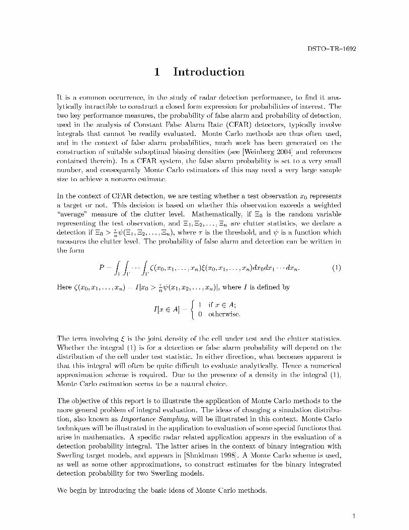
1 Introduction

It is a common occurrence, in the study of radar detection performance, to find it ana-lytically intractible to construct a closed form expression for probabilities of interest. Thetwo key performance measures, the probability of false alarm and probability of detection,used in the analysis of Constant False Alarm Rate (CFAR) detectors, typically involveintegrals that cannot be readily evaluated. Monte Carlo methods are thus often used,and in the context of false alarm probabilities, much work has been generated on theconstruction of suitable suboptimal biasing densities (see [Weinberg 2004] and referencescontained therein). In a CFAR system, the false alarm probability is set to a very smallnumber, and consequently Monte Carlo estimators of this may need a very large samplesize to achieve a nonzero estimate.

In the context of CFAR detection, we are testing whether a test observation x0 representsa target or not. This decision is based on whether this observation exceeds a weighted"ý'average" measure of the clutter level. Mathematically, if B0 is the random variablerepresenting the test observation, and B1 , B2 ,..., B.n are clutter statistics, we declare adetection if B0 > ý'(EB1, B2, .... , 7n), where T is the threshold, and ýb is a function whichmeasures the clutter level. The probability of false alarm and detection can be written inthe form

P zz "jf..j (x°xI ... 'xn)ý(xOxl,..."xn)dxodxl"..dx. (1)

Here ((xO0X1, ... ,Xn) I[XO > nxl, X2,..., Xn)], where I is defined by

[X c A] 1 ifxcA;

0 otherwise.

The term involving ý is the joint density of the cell under test and the clutter statistics.Whether the integral (1) is for a detection or false alarm probability will depend on thedistribution of the cell under test statistic. In either direction, what becomes apparent isthat this integral will often be quite difficult to evaluate analytically. Hence a numericalapproximation scheme is required. Due to the presence of a density in the integral (1),Monte Carlo estimation seems to be a natural choice.

The objective of this report is to illustrate the application of Monte Carlo methods to themore general problem of integral evaluation. The ideas of changing a simulation distribu-tion, also known as Importance Sampling, will be illustrated in this context. Monte Carlotechniques will be illustrated in the application to evaluation of some special functions thatarise in mathematics. A specific radar related application appears in the evaluation of adetection probability integral. The latter arises in the context of binary integration withSwerling target models, and appears in [Shnidman 1998]. A Monte Carlo scheme is used,as well as some other approximations, to construct estimates for the binary integrateddetection probability for two Swerling models.

We begin by introducing the basic ideas of Monte Carlo methods.

DSTO-TR-1692

2 Monte Carlo Techniques

The application of simulation methods to the estimation of difficult integrals began withthe work of [Kahn 1950] and others working in nuclear physics in the 1940s. An earlyradar application to estimation of false alarm probabilities is [Mitchell 1981]. The basisfor Monte Carlo techniques is the Strong Law of Large Numbers (SLLN) (see [Billingsley1986]). This states that a series of independent and identically distributed (IID) randomvariables, normalised by the number of terms in the series, will converge to the mean ofany one of the terms in the series. Mathematically, this implies that if 1 , B2 ,..., E7 is asequence of IID random variables with finite mean E[B], then

lim j-1 E[B], (2)---- Tm

except on a set of probability measure zero. This suggests that, for sufficiently large m,the average of the random variables in (2) can be approximated by its mean. Where thisapplies, in the context of interest, is that it enables the evaluation of integrals throughsimulation.

Consider the integral I fQ w(x)ý(x)dx, where ý is a density on Q, and w is a function.This integral is a statistical mean of a random variable B on Q with density ý. Hence wecan write I E[w(B)]. Now if B 1 ,BE2 ,..., EmT is an IID sequence of random variables,then the SLLN (2) implies that

lim j-1 E[w(BE)] I, (3)m--c •m

except on a set of probability measure zero. Hence, by applying (3), we can deduce that

m

I 1 w(x)t(x)dx j1 m (4)

where the sequence Z1 , z 2 ,... , Zm consists of realisations of the variables B1 , B2 ,... , "m.

The result in (4) implies that the integral I can be estimated by generating a seriesof realisations of a random variable with density ý, and evaluating the average of thefunction w over these realisations. This is a computationally simple exercise in theory.As remarked previously, an underlying problem with Monte Carlo methods is that it mayrequire a very large sample size to achieve a reasonable estimate. Changing the biasingdensity can sometimes rectify this, and this will be considered in the discussion to follow.

In cases where we have a definite integral of a function that is not a density on the integral'sdomain, it is still possible to apply Monte Carlo methods. To illustrate this, suppose I isa definite integral of the form

f ((x)dx, (5)JA

DSTO-TR 1692

where ( A -* R is a continuous nonnegative real valued function on the interval A -

[a, b]. We do not assume that the boundaries of this interval are finite, so that we allowfor integrals on infinite domains. We do assume, however, that the integral exists, in aRiemann or Lebesgue sense. We would like to apply the SLLN to (5), in order to apply aMonte Carlo approximation. We can construct a probability density function ý on A, andmodify the integral to

IA ( x)dx Fw(B), (6)

where w(x) and the expectation in (6) is with respect to a random variable " with

density ý. We require this density to be nonzero so that w(x) is well defined. The existenceof such densities can be shown by considering the four types of integral domains. If theintegral's domain is an interval of the form [a, b], where both a and b are finite, then onecan choose a uniform distribution over this domain. In the case of an integral with domain[a, cc) or (-oo, b], where both a and b are finite, an Exponential distribution can be used.The final case, where the integral is over the whole real line, a Gaussian distribution canbe used. This procedure is often referred to as Importance Sampling. [Weinberg 2004]contains a detailed list of Importance Sampling references.

An application of the SLLN to (6) results in the Monte Carlo estimator

IN N Z ct(h), (7)j=1"

dd

where each ",j - E. In general, the expression 4) d T means that the distributionsof random variables 4) and T are equal, so that for every set A in a common domain,P(J) c A) - P(I c A). Estimator (7) is an unbiased estimator of I, since

FIN IEw(B) fw(x)t(x)dx I1. (8)

Thus estimates are centred on the integral being approximated. The variance of (7) can

be shown to be

VINA xl (IE(w(B•)2) - (IE(w(B•))2)

We would like to have an estimator whose variance is as small as possible. Notice thatwith the choice of •(x) on A, the variance (9) reduces to zero. This biasing density

VIN

is known as the optimal solution, but is of no practical use because it depends on thequantity being estimated. Many authors have used knowledge of the optimal solution toconstruct a suboptimal biasing density, with varying degrees of success (see [Gerlack 1999]and [Orsak and Aazhang 1989]). Its form suggests that a suitable biasing density shouldbe concentrated on the integral's domain, and in some sense proportional to the integrand.

withthechoce f ýx) (() onA, he arince(9)redces o zro.Thi bisin desit

DSTO-TR-1692

Thus, if we are presented with an integral of the form (5), there are three ways to proceedin terms of the Monte Carlo approach. If integrand ((x) contains a density on the integral's

domain, we can use this to simulate. If this is not the case, then we can insert a biasingdensity, and alter the integrand. The other possibility is that we can change biasingdensities even if ( does contain a density.

We now turn to the issue of a suitable choice of biasing density. There are many differentdistributions from which one can select a biasing distribution. The Weibull family of

distributions, W(a, /), with nonnegative parameters a and /3, has probability densityfunction

Sw(x) a

and can be simulated via

%7 j(R) /3(-log(R))U dW(a,/3),

where I)w(x) is the cumulative distribution function, and R d R(O, 1) is a continuous

uniform distribution on the unit interval. There are a number of important special casesof the Weibull distribution. Observe that W(1, /3) is an Exponential distribution, whileWV(2, /3) is Rayleigh.

The Gamma family of distributions, g(r, /3), has density

( r-1 x

where 7(r) is a normalising constant, called the Gamma function, and we also assumeparameters r and /3 are nonnegative. It is analytically impossible to write down theinverse of the cumulative distribution function of the Gamma distribution. However,

it is possible to simulate from this distribution, using the fact that if B is a randomvariable with the Gamma distribution with parameters r and /3, then B "El + B2 +

+Br, where each "Bj is an IID Exponential random variable with parameter /3. Thusrealisations of a Gamma distribution can be obtained by summing independent realisationsfrom Exponential distributions.

The success of a biasing density is largely application dependent. In the next sectionwe will investigate the result of applying different biasing densities to the Monte Carloestimation of some special functions.

4

DSTO-TR 1692

3 Monte Carlo Approximations of some SpecialFunctions

In order to illustrate the application of Monte Carlo simulation to the evaluation of inte-grals, we examine two special functions. The Gamma and Beta functions arise in a numberof contexts in mathematics and statistics. In applied mathematics, these functions appearin the theory of Bessel functions [Bowman 1958]. They arise as normalising constants inthe definition of certain distributions in the theory of probability [Ross 1983]. The Gamma

function 7(n) WR --* R is defined by the integral

" "y(j) xn-le-xdx, (10)

and the Beta function /(m, n) : R+ x W- R is01J3(m, n) xm

1 (1 -_ x)n-ldx. (11)

For nonnegative integral n, it can be shown that 7(n + 1) n!. The Beta function can bedecomposed into an ex]pression involving Gamma functions. Specifically, it can be shownthat J3(m, n) - .'((n. Except for some simple cases, it is necessary to use numericaly(m-+n)*methods to evaluate these integrals in practice. We will apply Monte Carlo techniques toboth (10) and (11). In the case of (10), the exponential term ý(x) : ex is a density onthe interval [0, oo). Hence, an appropriate Monte Carlo estimator of (10) is

I N

(n, N) +NZBE (12)j=1

where each E is a random variable generated from a distribution with density ý. In thiscase, since ý is the density of an Exponential random variable with parameter 1, we can

SduseB log(R) to simulate the distribution, where R is a uniform density on the interval[0,1].

We can construct an alternative estimator by simulating from a distribution with density

from the Weibull class. If ý is the Weibull density ý(x) ((- , then an

estimator based on this is

F2(n, N) N j Bj- ý(z j)j=1"

e ± ()o (13)aN

j=1

where each BE j3(-log Rj)o, with Rj d R[0, 1].

Figures 1-3 in Appendix A contain simulations to estimate the Gamma function, usingboth the estimators (12) and (13). The Matlab code used to generate the estimates can be

5

DSTO-TR-1692

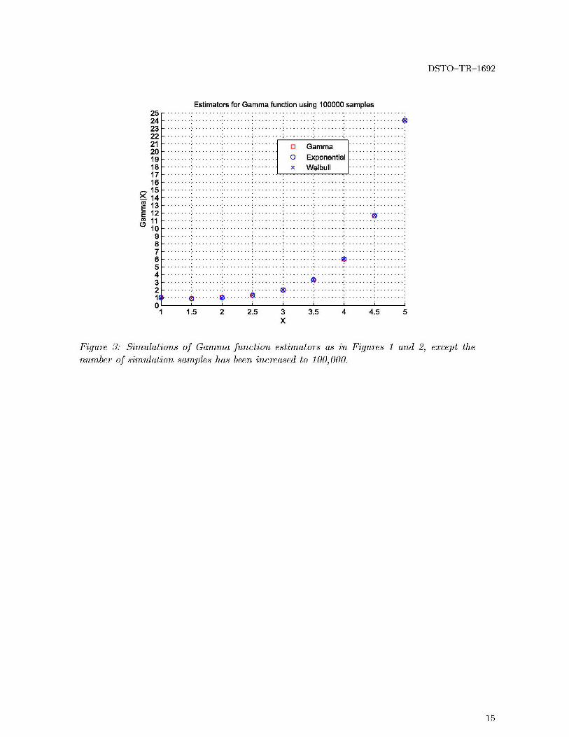
found in Appendix B. Each plot compares these two estimators to the exact value for theGamma function, or a numerical approximation based upon an inbuilt Matlab function.Figures 1 and 2 are based upon a sample size of N 10, 000, while that of Figure 3 isbased upon a sample of size of N 100, 000. The Weibull estimator (13) was chosen withparameters a 1 and /3 10. It was found empirically that other values for a did notprovide good estimates. The simulations show there is reasonably good convergence tothe exact value for approximately 100,000 simulation runs.

The Beta function can also be estimated using Monte Carlo estimators. The difference isthat the domain of the integral is the unit interval [0, 1]. A suitable density on this intervalis the standard uniform one, which is ý(x) 1, for x c [0, 1]. In this case, the MonteCarlo estimator is A 1 N

--mny), N) 7Z l (1Bj)n 1 , (14)/31(7•,?,N) N I: ?-I( n-

j-1

where in this case, each "-j is a random variable with the standard uniform density on[0, 1]. There are also some other natural choices for biasing densities for the Beta function.We can choose ý(x) mxm-l, and introduce a scaling factor of m to the Beta function'sintegral. Hence the estimator is

2 (m, nN) _ Z1 _ 7j)n, (15)mN (-1 - -1

where E is a random variable with the density ý. This can be simulated from the fact

that R ", where R - R[0, 1] is a uniform distribution on the unit interval. Note thata biasing density can also be based on the second term in the integrand. Specifically, wecould make the choice of ý(x) n(1 - x)n- 1 , which is also a density on the unit interval.

As remarked in Section 2, it is possible to simulate from any distribution we can defineon the integral's domain. In the current context, we could insert a modified Exponentialdistribution into the Beta integral, and use this for simulation. To illustrate, note thatthe function ý(x) -%1 is a density on [0, 1], and a random variable B with this as its

density can be simulated by - log(1 - (1 - e- 1 )R) d "E where as before R is the standarduniform distribution on the unit interval. This distribution is referred to as a truncatedExponential distribution. Thus a third estimator of the Beta function is

/33 (M I n, N) 1 -- I-1 NN Z) , (16)j=1

where "Bj is generated from the truncated Exponential distribution.

Figures 4-6 in Appendix A contain a number of simulations of the three estimators (14)-(16). For given values of m and n, these estimators are compared to the exact result.In contrast to the estimates for the Gamma function, there is rapid convergence in thiscase. After only 100 simulations, the estimators are giving very good estimates of the Beta

function.

6

DSTO-TR 1692

4 Monte Carlo Approximations of DetectionProbabilities

We now turn to the problem of estimating radar detection probabilities using Monte Carlomethods. The detection probability under consideration arises in the context of binaryintegration for Swerling target fluctuations [Shnidman 1998]. As an alternative to coherentintegration of N pulses [Levanon 1988], binary integration determines how many singlepulse exceedences of the threshold occur. A target detection is declared if there are atleast M such exceedences, for a prescribed value of M, within N observations. A keyissue is to determine the optimal value of M, which is the focus of [Shnidman 1998]. Wewill instead assume such an optimal value has been determined, and will investigate thecorresponding detection probability integrals.

The following is taken from [Shnidman 1998], with slight modification of notation. Definethe cumulative distribution function of Binomial probabilities between two integers N andM, with 1 < M < N, to be

E(N,M,p)r S�(N) (1 -p)N-kpk, (17)k-M

for some 0 < p < 1. The binary false alarm probability is PFA E(N, M, pi), where

Pi is the single pulse false alarm probability. The single pulse normalised threshold isT - log(pl). We define " to be the target normalised signal to noise ratio (SNR), whichunder Swerling models, we assume has a Gamma distribution with parameters r 1 and0 ý ý. The parameter 1 is a fluctuation parameter, and ýo is the average normalised

SNR. The density of B is thusPl-1 (0l I

ý(t14,'l) - e- Co. (18)

We let p,(t, T) be the single pulse probability of detection, for a constant target with single

pulse normalised SNR level t. Then

p,(t, T) e-(t 2vt)dv

6 -Q7-t) j0 e7-I0(2 (v + T)t)dv, (19)

where j0 is the modified Bessel function of order zero [Bowman 1958]. For the fourSwerling target models considered in [Shnidman 1998], the binary integrated probabilityof detection turns out to be

PD f E(N,M,p(t, -))ý(tj~o,l)dt, (20)

where the form of p(t, T) depends on the Swerling case. As explained in [Shnidman 1998],for Swerling 1 and 3, p(t, T) p,(t, T). In the case of Swerling 2,

p(t, T) ]P,(P, -)ý(Pjo,l 1)dp e1mo, (21)

7

DSTO-TR-1692

where the latter equality can be demonstrated analytically. It is important to note thatthe fluctuation parameter 1 is taken to be 1, for Swerling 1 and 2 target models, and isassumed to be 2 for Swerling cases 3 and 4. In the case of Swerling 4,

p(t,T) fP,(P, T)ý(PlýO,1 2)dp, (22)

the difference between this and (21) being the difference in fluctuation parameters. Whenapplied to (20), the Swerling 2 and 4 expressions for p(t, T) do not depend on t, and so (20)reduces to the cumulative sum of binomial probabilities (17). Hence we do not examinethese cases further, since Monte Carlo simulations are not required. We would like toobtain estimates of (20), using a Monte Carlo approximations, for Swerling 1 and 3 targetmodels.

The presence of the Gamma density in (20) suggests that this could be used as a simulationdensity. Hence, a Monte Carlo estimator for the detection probability (20) is

1K

PD (N, M, K, T) - .i E(N, M, P, (Ej, T)), (23)j-1

where each Bj is a Gamma random variable with density given by (18). The Gammavariables can be simulated by adding r - 1 independent realisations of Exponential randomvariables with parameter 3 .

We now need to approximate p,(t, T). There are two possiblities. Firstly, from [Shnidman1995] and [Weinberg and Kyprianou 2005], we have

00 tk Tj

p,(t, T) e-(T+t) E E --k-0k .-O

e-(T+t) x

(24)

1+t(1+T)+- 1+T+- +- 1+T+-+- ..

which yields the approximation

log(p,(t, T)) -T + Tt - T + 2 - (25)

Note that this quadratic expression is always negative which is important since p,(t, T) isa probability, and any estimate of it must also be a probability.

We would expect the approximation (25) to not work well except when t and T are bothsmall.

8

DSTO-TR 1692

Secondly, from [Weinberg and Kyprianou 2005], we have

p -(t,) P(N 2(T) •< Nl(t)), (26)

where (N1(t), N2(T)) d (Po(t), Po(T)) are independent Poisson random variables. (Notethat Po(A) indicates a Poisson distribution with mean value A).

A Monte Carlo estimator of (19) can be based on (26), by simulating from the distributionof N, and evaluating cumulative probabilities of N2. Specifically, one can use the estimator

1H

fr(t, T) HZ P(N2(T) _< ), (27)j=1

where each Qj is generated from a random variable with a Po(t) distribution. This can beused in conjunction with the estimator (23) to estimate the detection probability (20). Itwas found that an estimator based on (27) converged faster, and for less simulation runs,than an estimator based directly on the integral (19). Using (27) also provided better sim-ulation estimates for the probability (20), rather than using the quadratic approximation(25).

Figure 7 in Appendix A is a simulation of (23), in the case where N - 5, M - 3,1 - 2, ýo 1 and T - 0.4. The estimator's Matlab code can be found in Appendix B.The quadratic approximation (25) was used to estimate the probability (19). The jthsimulation uses K - 10 iterations in the estimator (23). As can be observed, the MonteCarlo estimator (23) begins to settle down from the third simulation, which correspondsto K 1000.

Figures 8-11 in Appendix A contain a number of simulations of the estimator (23), compar-ing the usage of the quadratic approximation (25) to the Poisson estimator (27). Figures8 and 9 are for the case where N 7, M 3, 1 - 2, 0o - 0.001 and - 1. The jthsimulation uses K 10i. Figure 8 compares an estimator using the quadratic approxima-tion (25) to one using the Poisson estimator (27), with H - 1000. In this example, bothestimators seem to be settling down after K - 1000 simulations. Figure 9 is for the samescenario, except only estimators based upon the Poisson estimate (27) are included. Thethree cases considered are for H - K, H - 10 and H - 1000. This simulation, as well asothers investigated, showed that it is sufficient to take around H - 1000 to obtain a goodPoisson estimate.

Figure 10 is a simulation for the case where N - 5, M - 3, 1 - 2, ýo 1 and T - 5.3704.As previously, K 10i for the jth simulation. Three estimators are compared to anapproximation based upon a numerical integration scheme1 . The numerical integrationscheme gave a detection probability of 0.0095. The two Poisson estimators use H - Kand H - 1000 respectively. As can be observed, the Poisson based estimates coincide withthe numerical value rather quickly, while the quadratic based estimator improves slowly.

1 This was provided by Mr Daniel Finch, EWRD, who used Matlab's numerical integration functionquad to estimate the detection integral (20).

9

DSTO-TR-1692

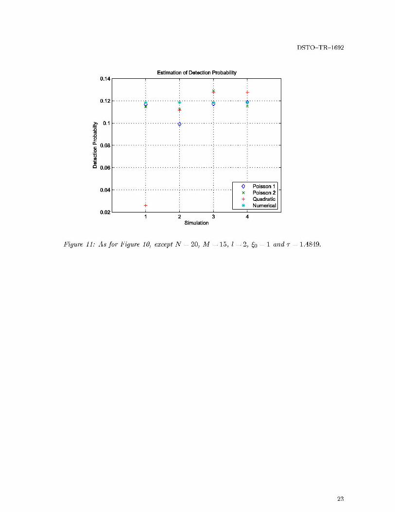
Figure 11 contains estimates for the case where N - 20, M - 15, 1 - 2, ýo 1 andT - 1.4849. The three estimators used are the same as in Figure 10. The numericalscheme gave a value of 0.1184. In this case, the Poisson estimator with H - K has the

best performance.

Other simulations considered showed that the estimator (23), when coupled with the

quadratic approximation (25), had very poor performance when the threshold T and theSNR ýo were fairly large. In contrast to this, it was found that using the Poisson estimate(27) improved the estimation considerably, with reasonable results for K - 1000.

10

DSTO-TR 1692

5 Conclusions and Future Directions

This report examined the Monte Carlo estimation of definite integrals. A number ofestimators of the Gamma and Beta function were considered. These estimators performedreasonably well in practice. A number of estimators of the probability of detection, for abinary integration scheme, were also considered. These gave reasonable results in practice.

In future work, the detection probability estimator will be compared to other estimators,to gauge its performance.

Acknowledgements

Thanks are due to Dr Hatem Hmam, Dr Brett Haywood, Dr Andrew Shaw and Dr ArisAlexopoulos, for reviewing the report. We also thank Mr Nick Lioutas for drawing at-tention to the problem of estimating binary integration detection probabilities, and MrDaniel Finch for giving us access to his Matlab code. We are also grateful to the CEWRDDr Len Sciacca for having a sincere interest in our research endeavours.

11

DSTO-TR-1692

References1. Billingsley, P (1986), Probability and Measure, John Wiley and Sons, 2 nd Ed.

2. Bowman, Frank (1958), Introduction to Bessel Functions. Dover, New York.

3. Courant, R. and John, F. (1965), Introduction to Calculus and Analysis, VolumeOne. Wiley, New York.

4. Gerlach, K. (1999). New Results in Importance Sampling. IEEE Trans. Aero. Elec.Sys., Vol. 35, No. 3, pp. 917-925.

5. Kahn, H. (1950), Random Sampling (Monte Carlo) Techniques in Neutron Attenua-tion Problems-I. Nucleonics, pp. 27-37.

6. Levanon, N. (1988), Radar Principles. John Wiley & Sons, New York.

7. Mitchell, R.L. (1981), Importance Sampling applied to simulation of false alarmstatistics, IEEE Trans. Aero. Elec. Sys. Vol AES-17, pp. 15-24.

8. Orsak, G. and Aazhang, B. (1989), On the Theory of Importance Sampling Appliedto the Analysis of Detection Systems. IEEE Trans. Comms, Vol. 37, No. 4, pp.332-339.

9. Ross, Sheldon (1983), Stochastic Processes. Wiley, New York.

10. Shnidman, D. (1995), Radar Detection Probabilities and their Calculations, IEEETrans. Aero. Elec. Sys. Vol 31, pp. 928-950.

11. Shnidman, D. (1998), Binary integration for Swerling target fluctuations, IEEETrans. Aero. Elec. Sys. Vol 34, pp. 1043-1053.

12. Tsypkin, A. G. and Tsypkin, G. G. (1988), Mathematical Formulas: Algebra, Geom-etry and Mathematical Analysis. Mir Publishers, Moscow.

13. Weinberg, G. V. (2004), Estimation of False Alarm Probabilities in Cell AveragingConstant False Alarm Rate Detectors via Monte Carlo Methods, DSTO TR-1624.

14. Weinberg, G. V. and Kyprianou, R. (2005), Estimation of Detection Probabilities

using Monte Carlo Sampling, to be submitted IEEE Trans. Aero. Elec. Sys.

12

DSTO-TR 1692

Appendix A: Simulations

Estimators for Gamma function using 10000 samples25 ......................................... .........2 4 . . . . . . .. .. . . . . . . . .... . . . . . . . . . . . . . . . . . . . . . . . . . . . . . . . . . . . . . . . . . . . . . . . .23 ................ ........................... .........2 2 .. . . . . . . ... . . . . . . . ... . . .. " . . . . . . . . . . . . . . . . . . . . . . . . . . . . . . . .... . . . . . . . .2 1 .. ...... :.................. ..... . ......m .........20 .............. ..........19 ....... ........................ 0 Exponential ............18 .... ....................... ...... x W eibull17 ...................... . . . ......16........ ................... ......................15 ....................................................

- 14 ......... ......... ........ ..........1 3 . . . . . . .. . . . . . . . . . .. . . . " .. ... . . . . . . . .. . . . . . . . .

. . . . . . . . . . . . . . . . . . . : . . . . . . . . .E 1 2 . .. . . . ... :. . . . . . . .. :. . . . . . . . .... . . . . .. .; . . . . . . .. :. . . . . . . . .:. . . . . . . . . . . . . . . . ..

.. .. . . . . .. : . . . . . . . . .: . . . . . . . .". . . . . . . . . ." . . . . . . . .: . . . . . . . . .: . . . . . . . .: . . . . . . . .

8 . . . . . . .. .. . . . . . . . ... . . . . . . . : . . . . . . . . . . . . . . . . ... . . . . . . .... . . . . . . . : . . . . . . . . .7 . . . . . . .. .. . . . . . . . .:... . . . . . . . . . . . . . . . . . . . . . . . . . . . . .8 ... . . . ... :. . . . . . . .. :. . . . . . . . .. ... . .. . . . .; . . . ... . .: . . . . . .. .® . . . . . . . .. . . . . . . .:7 . . . . . . . .. .. . . . . . .. .. . . . . . . . . . . . . . . . . . . . . . . . . .. . . . . . . ... . . . . . . . . . . . . . . .. .6 .. ................... . . . . .......... ..............0 ...... ......5 .. .. . . . .. . . . . . . . . . . . .. . . . .. . . . .. . . ... . . .

4 . . . . . . . .. . . . . . . . .. . . . . . . . .. . . . . . . . . . . . . . . ..... .. . . . .0 .. . . . . . . :

12 . . . . ... ... . . . . .. .... . . . . .. . . . . . . . . .0 . . . . . . . .:. . . . . . . . .:. . . . . . . .. : . . . . . . . ..:

01 1.5 2 2.5 3 3.5 4 4.5 5

X

Figure 1: Simulations of the Gamma estimators (12) and (13), for a selection of valuesof X. In each case, both estimators are compared with an estimate based on the Matlabinbuilt Gamma function. The number of simulations used in each case is 10,000. In thelegend, Gamma refers to the exact result, Exponential refers to the estimator (12) andWeibull refers to (13).

13

DSTO-TR-1692

Estimators for Gamma function using 10000 samples25 ......................................... .........2 4 . . . . . . .. .. . . . . . . . .: .. . . . . . . . . . . . . . . . . . . . . ..... . . . . . ..... . . . . . . . . . . . . . . .23................ .......... :.....................2 2 .. . . . . . . ... . . . . . . . ... . . .. " . . . . . . . . . . . . . . . . . . . . . . . . . . . . . . . .... . . . . . . . .21....................... . . Gamma.. .................20 ........................

19 ....... ........................ 0 Exponential ............18 .... ....................... ...... x W eibull17 .... .................. . . . ......16.................. ..................................15 ....................................................

X - 1 4 .. . . . . .. .. . . . . . . . . . . . . . . . . . . . . . . . . . . . . . . . . . . . . . . . . . . . . . . . . . . . . . . . . .'0 13 ..... .. ........................... . ........E 12 .... ........ ...... . . ............................ . ...... .........S1 1 . . . . . . ..... . . . . . . . . . . . . . . . . . . . . . . . . . . . . . . . . . . . . . . . . . . . .

10 ............................................ ........9 . . . . .. . . .. . ... . . . . . . . . . . " . . . . . . . . . . . . . . . . . . . . . . . . . . . . . . . . .8 ..... .. . . . . . . . . . . . . . . . . . . ... .. . . . . .. : . . . . . . . .. :. . . . . . . . .... . . . . .. .: . . . . . . . .. : . . . . . . . .. :. . . . . . . . .. . . . . . . .

. . . . . . .. . . . . . . . .. . . . . . . . . . . . . . . . . . . . .5 . .. . . .. . . . . .. . .. . . . . .. . . . . . . . . . . . . . . . . .. . ... . . . . . . . .. . . . . . . . . . . . . . . . . . .

5 . . . . . . .. .. . . . . . . . .:. . . . . . . . : . . . . . . . . :.. . . . . . ... . . . . . . . . . . . . . . . . . '. . . . . . . ..5 . . . . : . . . . ...... . . . . . ... . . . . . . . . . . . . . . ..2 . . . .:.. . . . ... . :.. . . . . .. "®.. . . . . . . :. . .... . . . . . . .. . . . . . . . . . :4 ... .. .. .. ... .. .. .. .

12 . . . . ... .... . . . . .. .... . . . . .. . . . . . . . . .e: . . . . . . . .:.. . . . . . . . :... . . . . .. . . . . . . . . ..:0** 0 i i01 1.5 2 2.5 3 3.5 4 4.5 5

X

Figure 2: A simulation under exactly the same conditions as that of Figure 1, showingslightly worse results.

14

DSTO-TR 1692

Estimators for Gamma function using 100000 samples25 ..................................................2 4 .. . . . . .. .. . . . . . . . .: .. . . . . . . . . . . . . . . . . . . . . ..... . . . . . ... .. . . . . . . . . . . . . . .23................ .......... :.....................2 2 .. . . . . . . ... . . . . . . . ... . . .. " . . . . . . . . . . . . . . . . . . . . . . . . . . . . . . . .... . . . . . . . .21 . ....... . .......... ........ .................... G am m a20 ........................

19 ....... ........................ 0 Exponential............18 .... ....................... ...... x W eibull17 .... ................. . .. . ..... .

16.................. ..................................15 ....................................................

- 1 4 .. . . . . .. .. . . . . . . . . . . . . . . . . . . . . . . . . . . . . . . . . . . . . . . . . . . . . . . . . . . . . . . . . .0E 1 3 .. . . . . .. .. . . . . . . . ... . . . . . .. . . . . . . . . . . . . . . . ... . . . . . . . .. . . . . . . .. . . . . . . . ..E 1 2 .. . . . . . :... . . . . . . . :... . . . . . .. . . . . . . . . . :.. . . . . . . . :... . . . . . .. .. . . . . . . .® . . . .

S1 1 . . . . . . . :. ... . . . . . .... . . . . . . . ; . . . . . . . . .; . . . . . . . . .: . . . . . . . . .: . . . . . . . . . . . . . . . ..101 0 . . . . . . .. .. . . . . . . . .:. . . . . . . .. : . . . . . . . . :. . . . . . . . :. .. . . . . . .. .. . . . . . . . . . . . . . . ..:

8 . . . . . . .. .. . . . . . . . .i. . . . . . . . ". . . . . . . . i. . . . . . . . ..i . . . . . . . . .i. . . . . . . . !. . . . . . . .. i9 . . . . . . . ... . . . . . . . ... . . . . . . . . ... . . . . . . . . . . . . . . . .. . . .. . . . . . . .: . . . .. . . . . . . . .

7 . . . . . . . .. .. . . . . . .. .. . . . . . . . . . . . . . . . . .. . . . . . . .. .. . . . . . .. .. . . . . . . . . . . . . . . . .. . . . . . . . . .. . . . ..6. . .. . . . .. . . . . . . . . . .. . . . . . . . . . . . . . . . . : . . . . . . . . . . . . . . .5 . . . . . . . . . . . . . :. . . . . . . . ". . . . . . . . :.. . . . . . . . . . . . . . . . . . . . . . . . . . . . . . .4 -..... ... .. .. .. ..

3 .. . . . .. . .. . . ..... .... .. .. . .. .. .. . .. .12 . . . . ... .... . . . . .. .... . . . . .. . . . . . . . . .0 . . . . . . . .:.. . . . . . . . :. . . . . . . .. : . . . . . . . ..:1*** .. .. . .. 0 .. . . .. . ..

01 1.5 2 2.5 3 3.5 4 4.5 5X

Figure 3: Simulations of Gamma function estimators as in Figures 1 and 2, except the

number of simulation samples has been increased to 100,000.

15

DSTO-TR-1692

Estimators for Beta function using 50 samples1.4-

1.2

0 Beta

+ 0 Uniform

X Polynomial

+ Exponential

S0 .8 - . . . . . . . . . . . . . . . . . . . . . . . . . . . . .. . . . . .... . . . . . . . . . . . . . . . . . . . . . . . . . . . . . .

E

08

0 . .. . . . . . . . . . . . . . . . . . . . . . . . . . . . . . . . . . . . . . . .. . . . . . . . . . . . . . . . . . . . . . . .. . . . . .

0.4-

0 .2 . . . . .... . . . . . . .. . . . . . . . .. . . . . . . . . .. . . . . . . . . . .. . . . . . . . . ... . . . . . . . . ... . . . . ... . . . . . . . . . . . . . . . . . . .

02I II I I I I I I

(11) (1,2) (1,3) (2,1) (2,2) (2,3) (3,1) (3,2) (3,3)(nm)

Figure 4: Simulations of the Beta integral estimators (14), (15) and (16). In each case,50 simulations have been used to estimate the integral (11) with parameters (n, m). In the

legend, Beta refers to the exact result, while the other three refer to the estimators in orderof appearance.

16

DSTO-TR 1692

Estimators for Beta function using 100 samples1.4-

1.2 . ........

0 Beta

O Uniform

x Polynomial

+ Exponential

0 .8 . . . . . . . .... . . . . . . . . . . . . . ... . . . . . . . . . . . . . . . . . ..E

080 .6 . . . . . . . . . . . . . . . . . . . . . . . . . . . . . . . . . . . . . . . . . . . . . . . . . . . .

0 4 . .. . . . . . . . . . . . . . . . . . . . . . . . . . . . . . . . . . . . . . . .. . . . . . . . . . . . . . . . . . . . . . . . .0.4-

0 2 . . . . . . . . . . . . . . . . . . . . . . . . . . .... . . ... . . . . . . . . . . . . . . . . . ... . . . . . . . . . . . . . . . . . . .

020 C I I I I I I 1•I

(1,1) (1,2) (1,3) (2,1) (2,2) (2,3) (3,1) (3,2) (3,3)(n,m)

Figure 5: Same as for Figure 4, except 100 simulations are used to generate the estimates.

17

DSTO-TR-1692

Estimators for Beta function using 1000 samples1.4-

1.2 . ........

0 Beta

O Uniform1 . . .. .® . . . . . . . . . . . . . . . . . . . .. . . . . . . . . . . . . . . . . . . . . . . . . . . .

X Polynomial

+ Exponential

0 .8 . . . . . . . .... . . . . ... . . . . . . . . . . . . . . . . . ..E

0 6 . .. . . . . . . . . . . . . . . . . . . . . . . . . . . . . . . . . . . . . . . .. . . . . . . . . . . . . . . . . . . . . . . . .

0 4 . . . . . . . . . . . . . . . . . . . . . . . . . . . . . . . . . . . . . . . . . . . . . .. . . . . . . . . . . . . . . . . . . . . . . . .

0.2

04

* ®

S S

(1,1) (1,2) (1,3) (2,1) (2,2) (2,3) (3,1) (3,2) (3,3)(n,m)

Figure 6: As for Figure 5, except 1000 simulations are used.

18

DSTO-TR 1692

Estimation of Detection Probability0.015

0.0 140 .0 1 4 . . ... .. . . . . . . . . . . .. . . . . . . . . . . . . . . . . . . . .. . . . . . . . . . . .. . . . . . . . . . . . . . . . . . . . .

0 .0 1 3 - . . . . . . . . . . . . . . . . . . . . . . . . . . . . .. . . . . . . . . . . . . . . . . . . . . . . . . . . . . . . .

0 .0 1 2 . . . . . . . . .. . . . . . . . . . . .. . . . . . . . . . . . . . . . . . . . .. . . . ... . . . . . . . . . . . .

-• 0 .0 1 1 . . . . . .. . . . . . . . .. . . . . . . . . . . . . . . . . . . . .. . . . . . . . . . ... . . . . . . . . . . . . . . . . . .

0.013£

o _ 0 .0 0 1 . . . . . . . . . . . . . . . . . . .... . . . . . . . . . . . ... . . . . . . . ... ' . . . .0.012-~0

0 .0 0 7 . . . . . . . . . . .. . . . . . . . . .. . . . . . . . . . . . . . . . . . . . . . . . . . . . . . . . . . . . . .

0 .0 0 6 1...................

0.005

1 2 3 4 5 6Simulation

Figure 7: Simulation of (23) in the case of N 5, M 3, 1 2, ýo 1, T 0.4 and for

simulation j, K 10j. The quadratic approximation (25) was used to estimate the singlepulse probability (19).

19

DSTO-TR-1692

Estimation of Detection Probability0.987

0 Poisson0.9865 . ........ ....................... + Q uadratic

0 .9 8 6 . . . . . . . . . . . . . . . . . . . . . . . . . . . . . . . . . . . . . . . . . . . . . . . . . . . . . .. . . . . . . . . . . . .+

. , 0 .9 8 5 5 . . . . . . . . . . . . . . . . . . . . . . . . . . . . .

2 0.985-

0 0 .9 8 4 5 . . . . . . . . . . . . . . . . ... . . . . . ... . . . . . . . . . . .. . . . . . . . . . ..

o 0.984 . ........

0 .9 8 3 5 ............ ...........

0 .9 8 3 . . . . . . . . . . . . . . . . . . . . + . . . . . . . . . . .. . . . . . . . . . . . . .- . . . . . . . ..

0.98251 2 3 4 5

Simulation

Figure 8: A comparison of estimator (23) using the quadratic approximation (25) and the

Poisson estimator (27). In this case, N - 7, M - 3, 1 - 2, ýo - 0.001, T - 1. For eachj, K - 10J, and H - 1000.

20

DSTO-TR 1692

Estimation of Detection Probability

+ H=10

0.995 . ......................... ....... H = 1000

S 0 .9 9 - . . . . . . . . . . . . .... . . . . . : . . . . . . . . . . . . . . .. . . . . . . . . . . . .. + .. . . . . . . . . . . .

2.3 +

0- 0r- 0.995 +

o 0

o0.98

+0.975-

0.97' I I1 2 3 4

Simulation

Figure 9: Comparison of three estimators using different Poissons estimators. The sameparameter values are used as for the simulation of Figure 9, except the value of H is asshown.

21

DSTO-TR-1692

x 10.3 Estimation of Detection Probability14

* +

12 ...................................... ............

.• . 1 0 .. ....... . . . . . . . . . . . . . . . . . . . . . . . . ... . . . . . . . . . . . ..~1o......................... ....... ±

a)6' . . . . . . . . . . . . . . . . . . . . . . . . . . . . . . . . . . . . . . . . " . . . . . . . . . . . . . .. . . . . . . . . . . . .

46 .. . . . . . . . . . .. . . . . . . . . . . . . . . . . . . . . . . . . . . . . . . . . .

4........ . Poissoni1x Poisson 2

+ QuadraticNumerical

2i1 2 3 4

Simulation

Figure 10: A simulation in the case where N 5, M 3, 1 2, ýo 1 and T- 5.3704.As in previous simulations, K 10j. The first Poisson estimate uses H K, whilethe second uses H 1000. The numerical estimate is based upon numerical integrationapplied directly to the detection probability integral (20).

22

DSTO-TR 1692

Estimation of Detection Probability0.14

4 +0.12 ..................................... .........

_• 0 .1 .. . . . . . . . . . . . . . . . . . . . . . . . . . . . . . . . . . . . . . . . . . . . . . . . . . . . .. . . . . . . . . . . . . .-

0..

Ca

o0.06 ............ ............. ...........................n 0 .0 6 .. . . . . . . . . . . . . . . . . . . . . . . . . . . . . . . . . . . . . . .. . . . . . . . . . . . . . .. . . . . . . . . . . . . .-

S 0 .0 4 . . . . . . . . . . . . . . . . . . . . . . . . . . . . . . . . . . . . . . . . . . . . . . . . . . . . . . . . .

0.04. . Poisson 1x Poisson 2+ Quadratic

+ Numerical0.02 1'4

1 2 3 4Simulation

Figure 11: As for Figure 10, except N 20, M 15, 1 2, ýo 1 and T 1.4849.

23

DSTO-TR-1692

Appendix B: Matlab Code

-I, F EI I F -3 1 H MI

1 kunction Estimate = garocaEst(Option,N,a,b,Saoplee)

2 if nargin < 4

4 a= 1 ;

- b 1i ;

end!7

1% Different estimators of the gaona function

S switch Option

21 gaiaEst = @ ýo,o) gaosca~n)

2 c.ase I

I1 Sa -ples = -Ilg(Samples); 6 transform uniformly distributed samples to Exponential

14 gatrnaEst = @(x,n) sum(x.o(n-l))/leng9th(x);

15 ose 2

1- Samples = b.( -legiS•capleo (l . c/a); 0 transform uniforoly distributed samples to Weibull(a,

17 ganniEst = Iox,n) )(. ./c>~sua( o.)n-o)).Kecp)-+±(x./bj .cfl /length(.);

19

2 12 01;

21 fcrox 1:0.5:N2

22 cc + 1;

22 Estimate(m) = gsammaEst(samplesx);

24 end

41Ia.s P Is Ccl 1 701

Figure 12: This function calculates Matlab's Gamma function (Option 0), estimator (12)(Option 1) and estimator (13) (Option 2). N Gamma values are calculated for integersand half-integers from 1 to N. Parameters a and b correspond to the a and ,3 Gammaparameters. Samples is a vector of uniformly sampled points from the unit interval.

24

DSTO TR 1692

Eiie Edit Text Windoiw He lp

1 function Estimate = betaEst(Option,N,Samples,AsNatrix)

23 if nargin < 4

4 Asllatrix = false;

5 end

67 1 Different estimators of the beta function

8 switch Option

9 case 0

18 distn = @(u,m) 1"

11 betaF = U(x,m,n) beta(a,n);

12 case 1

1 distn = @(u,m) u;

14 betaE = 0(x,m,n) sum( x.A(T-l)).a((lx).A(n-I)))/length(x);

15 case 2

16 distn = 0(u,m) u.A(i/m);17 betaE = @(x,m,n) (i/m)lsum( ((l-x).I(n-l)))/length(x);

18 case 319 distn = @(u,m) -log(1-ý(i-exp(-I)) t

u));

20 betaE = U(x,m,n) sum((l-exp(-l)).texp(x).t(x.'(m-l)).t((l-x).'(n-1)))/length(x);

21 end

2 Estimate = zeros(N,N);

24 for a = I:N

25 for. n = i:N

26 Estimatecm,n) = betaE(distn(Samples,m),m,n),,

27 end

208 end

22 if -AsMatrix

30 Estimate = Estimate';

31 Estimate = Estimate :l;

32 end

FbetaEt LnO Cal

Figure 13: Function for calculation of Matlab's Beta function (Option 0), estimator (14)(Option 1), estimator (15) (Option 2) and estimator (16) (Option 3). N is an integer indi-cating the size of the matrix of Beta values. Samples is as for the Gamma implementationin Figure 12. AsMatrix, an optional argument, provides a better formatted output.

25

DSTO TR 1692

ile Edit Tt Window Help,

1 function Estimate = binintEst(Option, KI, K2, N, H, 1, xO, tau) t

3Sumn = 0;

4 for j=I:K1

5 t = gamrnd(1, xO/1);

h if Option == 17 Prob = sum(poisscdf(poissrnd(t,K2,I),tau))/K2;

H elseProb = (exp(-tau))*(1 + taunt - 0.5*(tau-0.5*tau'2);t'2);

112 end11

12 binSum = 0;

13 for i =M:N

14 binSum = binSum + binopdf(i, N, Prob);

1F end

15 Sum = Sum + binSum;17 end

18 Estimate = Sum/Kl;

41 I ,Ibinint~st Lnl 1. -:u ,Il

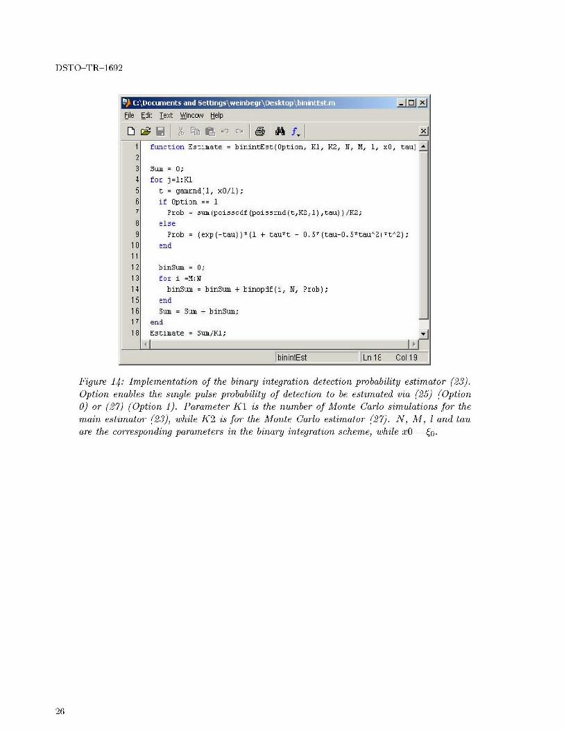
Figure 14: Implementation of the binary integration detection probability estimator (23).Option enables the single pulse probability of detection to be estimated via (25) (Option0) or (27) (Option 1). Parameter K1 is the number of Monte Carlo simulations for themain estimator (23), while K2 is for the Monte Carlo estimator (27). N, M, I and tauare the corresponding parameters in the binary integration scheme, while xO ýo.

26

DISTRIBUTION LIST

Approximation of Integrals via Monte Carlo Methods, with an Application toCalculating Radar Detection Probabilities

Graham V. Weinberg and Ross Kyprianou

AUSTRALIA

No. of copies

DEFENCE ORGANISATION

Task Sponsor

Commander, Maritime Patrol Group, RAAF Edinburgh 1

S&T Program

Chief Defence Scientist

FAS Science Policy

AS Science Corporate Management

Director General Science Policy Development

Counsellor, Defence Science, London Doc Data Sheet

Counsellor, Defence Science, Washington Doc Data Sheet

Scientific Adviser to MRDC, Thailand Doc Data Sheet

Scientific Adviser Joint 1

Navy Scientific Adviser Doc Data Sheet

Scientific Adviser, Army Doc Data Sheet

Air Force Scientific Adviser 1

Scientific Adviser to the DMO M&A Doc Data Sheet

Scientific Adviser to the DMO ELL Doc Data Sheet

Systems Sciences Laboratory

EWSTIS 1 (pdf format)

Chief, Electronic Warfare and Radar Division, Dr Len Sciacca Doc Data Sheet& Dist List

Research Leader, Microwave Radar, Dr Andrew Shaw Doc Data Sheet& Dist List

Task Manager, Dr Brett Haywood 1

Mr Nick Lioutas, EWRD 1

Mr Daniel Finch, EWRD 1

Author, Dr Graham V. Weinberg, EWRD 2

Author, Ross Kyprianou, EWRD 1

DSTO Library and Archives

Library, Edinburgh 1

Defence Archives 1

Capability Development Group

Director General Maritime Development Doc Data Sheet

Director General Capability and Plans Doc Data Sheet

Assistant Secretary Investment Analysis Doc Data Sheet

Director Capability Plans and Programming Doc Data Sheet

Director Trials Doc Data Sheet

Chief Information Officer Group

Deputy CIO Doc Data Sheet

Director General Information Policy and Plans Doc Data Sheet

AS Information Strategies and Futures Doc Data Sheet

AS Information Architecture and Management Doc Data Sheet

Director General Australian Defence Simulation Office Doc Data Sheet

Director General Information Services Doc Data Sheet

Strategy Group

Director General Military Strategy Doc Data Sheet

Director General Preparedness Doc Data Sheet

Assistant Secretary Governance and Counter-Proliferation Doc Data Sheet

Navy

Maritime Operational Analysis Centre, Building 89/90 Garden Doc Data SheetIsland Sydney NSW & Dist List

Deputy Director (operations) Doc Data Sheet& Dist List

Deputy Director (Analysis) Doc Data Sheet& Dist List

Director General Navy Capability, Performance and Plans, Doc Data SheetNavy Headquarters

Director General Navy Strategic Policy and Futures, Navy Doc Data SheetHeadquarters

Air Force

SO (Science), Headquarters Air Combat Group, RAAF Base, Doc Data SheetWilliamtown NSW 2314 & Exec Summ

Army

ABCA National Standardisation Officer, Land Warfare Devel- Doc Data Sheetopment Sector, Puckapunyal e-mailed

SO (Science), Land Headquarters (LHQ), Victoria Barracks, Doc Data SheetNSW & Exec Summ

SO (Science), Deployable Joint Force Headquarters (DJFHQ)(L), Doc Data SheetEnoggera QLD

Joint Operations Command

Director General Joint Operations Doc Data Sheet

Chief of Staff Headquarters Joint Operations Command Doc Data Sheet

Commandant ADF Warfare Centre Doc Data Sheet

Director General Strategic Logistics Doc Data Sheet

Intelligence and Security Group

DGSTA, Defence Intelligence Organisation 1

Manager, Information Centre, Defence Intelligence Organisa- 1 (pdf format)tion

Assistant Secretary Capability Provisioning Doc Data Sheet

Assistant Secretary Capability and Systems Doc Data Sheet

Assistant Secretary Corporate, Defence Imagery and Geospa- Doc Data Sheettial Organisation

Defence Materiel Organisation

Deputy CEO Doc Data Sheet

Head Aerospace Systems Division Doc Data Sheet

Head Maritime Systems Division Doc Data Sheet

Chief Joint Logistics Command Doc Data Sheet

Head Materiel Finance Doc Data Sheet

Defence Libraries

Library Manager, DLS-Canberra 1

Library Manager, DLS-Sydney West Doc Data Sheet

OTHER ORGANISATIONS

National Library of Australia 1

NASA (Canberra) 1

State Library of South Australia 1

UNIVERSITIES AND COLLEGES

Australian Defence Force Academy Library 1

Head of Aerospace and Mechanical Engineering, ADFA 1

Hargrave Library, Monash University Doc Data Sheet

Librarian, Flinders University 1

OUTSIDE AUSTRALIA

INTERNATIONAL DEFENCE INFORMATION CENTRES

US Defense Technical Information Center 2

UK Dstl Knowledge Services 2

Canada Defence Research Directorate R&D Knowledge & In- 1 (pdf format)formation Management (DRDKIM)

NZ Defence Information Centre 1

ABSTRACTING AND INFORMATION ORGANISATIONS

Library, Chemical Abstracts Reference Service 1

Engineering Societies Library, US 1

Materials Information, Cambridge Scientific Abstracts, US 1

Documents Librarian, The Center for Research Libraries, US 1

INFORMATION EXCHANGE AGREEMENT PARTNERS

National Aerospace Laboratory, Japan 1

National Aerospace Laboratory, Netherlands 1

SPARES

DSTO Edinburgh Library 5

Total number of copies: 39

Page classification: UNCLASSIFIED

DEFENCE SCIENCE AND TECHNOLOGY ORGANISATION 1. CAVEAT/PRIVACY MARKING

DOCUMENT CONTROL DATA

2. TITLE 3. SECURITY CLASSIFICATION

Approximation of Integrals via Monte Carlo Meth- Document (U)ods, with an Application to Calculating Radar De- Title (U)tection Probabilities Abstract (U)4. AUTHORS 5. CORPORATE AUTHOR

Graham V. Weinberg and Ross Kyprianou Systems Sciences LaboratoryPO Box 1500Edinburgh, South Australia, Australia 5111

6a. DSTO NUMBER 6b. AR NUMBER 6c. TYPE OF REPORT 7. DOCUMENT DATE

DSTO TR-1692 AR-013-341 Technical Report March, 20058. FILE NUMBER 9. TASK NUMBER 10. SPONSOR 11. No OF PAGES 12. No OF REFS

2005/1002553/1 AIR 01/217 CDR MPG 26 14

13. URL OF ELECTRONIC VERSION 14. RELEASE AUTHORITY

http://www.dsto.defence.gov.au/corporate/ Chief, Electronic Warfare and Radar Divisionreports/DSTO TR-1692.pdf

15. SECONDARY RELEASE STATEMENT OF THIS DOCUMENT

Approved For Public Release

OVERSEAS ENQUIRIES OUTSIDE STATED LIMITATIONS SHOULD BE REFERRED THROUGH DOCUMENT EXCHANGE, PO BOX 1500,EDINBURGH, SOUTH AUSTRALIA 5111

16. DELIBERATE ANNOUNCEMENT

No Limitations17. CITATION IN OTHER DOCUMENTS

No Limitations18. DEFTEST DESCRIPTORS

Monte Carlo Method, Radar detection, Detectionprobability, Integration19. ABSTRACT

The approximation of definite integrals using Monte Carlo simulations is the focus of the work pre-sented here. The general methodology of estimation by sampling is introduced, and is applied to theapproximation of two special functions of mathematics: the Gamma and Beta functions. A significantapplication, in the context of radar detection theory, is based upon the work of [Shnidman 1998]. Thelatter considers problems associated with the optimal choice of binary integration parameters. Weapply the techniques of Monte Carlo simulation to estimate binary integration detection probabilities.

Page classification: UNCLASSIFIED