Monte-Carlo Galerkin Approximation of Fractional ...downloads.hindawi.com/journals/mpe/2012/709106.pdfAbdallah Ali Badr1 and Hanan Salem El-Hoety2 1 Department of Mathematics, Faculty

Hindawi Publishing CorporationMathematical Problems in EngineeringVolume 2012, Article ID 709106, 14 pagesdoi:10.1155/2012/709106

Research ArticleMonte-Carlo Galerkin Approximation of FractionalStochastic Integro-Differential Equation

Abdallah Ali Badr1 and Hanan Salem El-Hoety2

1 Department of Mathematics, Faculty of Science, Alexandria University, Alexandria, Egypt2 Department of Mathematics, Faculty of Science, Garyounis University, Benghazi, Libya

Correspondence should be addressed to Abdallah Ali Badr, [email protected]

Received 30 November 2011; Accepted 2 February 2012

Academic Editor: Francesco Pellicano

Copyright q 2012 A. A. Badr and H. S. El-Hoety. This is an open access article distributed underthe Creative Commons Attribution License, which permits unrestricted use, distribution, andreproduction in any medium, provided the original work is properly cited.

A stochastic differential equation, SDE, describes the dynamics of a stochastic process definedon a space-time continuum. This paper reformulates the fractional stochastic integro-differentialequation as a SDE. Existence and uniqueness of the solution to this equation is discussed. A num-erical method for solving SDEs based on the Monte-Carlo Galerkin method is presented.

1. Introduction

Recently, many applications in numerous fields, such as viscoelastic materials, signal process-ing, controlling, quantum mechanics, meteorology, finance, and life science have been remo-deled in terms of fractional calculus where derivatives and integrals of fractional order is in-troduced and so differential equation of fractional order are involved in these models, see [1–5]. Generally, a fractional integro-differential equation with Caputo’s definition of fractionalderivative takes the form

uα(t) = f(t, u) +∫ tt0

h(t, s, u)ds, u(t0) = u0, t0 ≤ t ≤ T, 0 ≤ α ≤ 1. (1.1)

Also, in recent years, development of adequate statistical techniques for stochastic systemshas constantly been in the focus of scientific attention because of its outstanding importancefor a number of physical applications such as turbulence, heterogeneous flows and materials,

2 Mathematical Problems in Engineering

random noises, and so forth, see [6–8]. A stochastic integro-differential equation (SIDE) takesthe form

uα(t;w) = f(t, u;w) +∫ tt0

h(t, s, u;w)dWs, u(t0) = u0, t0 ≤ t ≤ T, 0 ≤ α ≤ 1, (1.2)

whereW is a Brownian motion.In this paper we study the FSIDE:

uα(t;w) +A(t)u(t;w) =∫ tt0

B(t, s;w)u(s;w)dWs + f(t;w), t > t0 (1.3)

with initial condition u(t0;w) = u0 and 0 ≤ α ≤ 1.The FSDE is a generalization of the fractional Fokker-Planck equation which describes

the random walk of a particle, see [9]. The aim of this paper is threefold. First we rewrite theabove equation as stochastic differential equation

du(t) = a(t, u;w)dt + b(t, u;w)dWs. (1.4)

Secondly we prove the existence and the uniqueness of the solution of this equation. Thirdlywe present a numerical method using finite element method and the Monte-Carlo method.

2. Preliminaries

In this section we collect a few known results to which we refer frequently in the sequel.Let Ω = {ω1, ω2, . . .} be the collection of all outcomes, ωi, i = 1, 2, . . . of an experiment,

and letA ⊂ Ω. Define themeasure P : A → [0, 1]with P(Ω) = 1. The triplet (Ω, A, P) is calleda probability space.

Definition 2.1. A collection {X(t, ·) : t ≥ 0} of random variables X : Ω × T → R, T = [0,∞] iscalled a stochastic process. For each point ω ∈ Ω, the mapping t → X(t, ω) is a realization,sample path, or trajectory of the stochastic process.

Definition 2.2. A real-valued stochastic process that depends continuously on t ∈ [0, T]W ={W(t), t ≥ 0},W : T ×Ω → R is called a Brownian motion (BM) or Wiener process if

(1) W(0) = 0 a.s.,

(2) W(t)−W(s) isN(0, t− s), the Gaussian distribution with mean 0 and variance t− s,for all t > s > 0,

(3) for all times 0 < t1 < t2 < · · · < tn, the random variables W(t1),W(t2) −W(t1), . . .,W(tn) −W(tn−1) are independents.

Also, the expected values ofW(t) andW2(t) are given by E(W(t)) = 0 and E(W2(t)) = t foreach time t > 0.

Definition 2.3. (i) Suppose that {At ≥ 0} is an increasing family of σ-algebras ofA such thatWt

is At-measurable E(W(t) | A0) = 0 and E(W(t) −W(s) | As) = 0 with probability one, w.p.1,for all 0 ≤ s ≤ t ≤ T .

Mathematical Problems in Engineering 3

(ii) Let L be the σ-algebra of Lebesgue subsets of R. Let L2T be a class of functions

f : [0, T] ×Ω → R satisfying the following:

(a) f is jointly L ×A-measurable;

(b)∫T0 E((f(t, ·))2)dt <∞;

(c) E((f(t, ·))2) for each 0 ≤ s ≤ t ≤ T ;(d) f(t, ·) is At measurable for each 0 ≤ t ≤ T .

Definition 2.4 (Convergence). If u(h) is the exact value of a random variable and un(h) is itsapproximate value, then we have

(1) strong convergence when

E(|u(h) − un(h)|) −→ 0, n −→ ∞, (2.1)

(2) weak convergence when

|E(u(h)) − E(un(h))| −→ 0, n −→ ∞, (2.2)

(3) mean square convergence when

E(u(h) − un(h))2 −→ 0, n −→ ∞. (2.3)

Definition 2.5. Let y(x) ∈ L1([a, b]), we define the fractional integral of order α, 1 ≥ α > 0, ofthe function y(x) over the interval [a, b] as

Jαa+y(x) =1

Γ(α)

∫xa

y(t)

(x − t)1−αdt, x > a,

Jαb−y(x) =1

Γ(α)

∫bx

y(t)

(t − x)1−αdt, x < b.

(2.4)

For completion, we define J0 = I (identity operator); that is, we mean J0y(x) = y(x).Furthermore, by Jαa+y(x) we mean the limit (if it exists) of Jαc as c → a+. This definition isaccording to Riemann-Liouville definition of fractional integral of arbitrary order α. For sim-plicity, we define the fractional integral by the equation

Jαy(x) =1

Γ(α)

∫xa

y(t)

(x − t)1−αdt, x > a, 0 < α ≤ 1, (2.5)

where we dropped a+. The folllowing equation

Dαy(x) =d

dxJ1−αy(x) (2.6)


denotes the fractional derivative of y(x) of order α. For numerical computations, we usuallyuse another definition of the fractional derivative, due to Caputo [2], given by

(CDαy

)(x) =

(Dα(y(t) − y(a)))(x). (2.7)

3. Formulation of the Problem

In this paper, we present a numerical method to solve the following FSIDE:

CDαt u(t;w) −A(t)u(t;w) =

∫ tt0

B(t, s;w)u(s;w)dWs + f(t;w), t > t0 (3.1)

with initial condition u(t0;w) = ut0 .For simplicity of notations, we drop the variablew, and so this equation takes the form

CDαu(t) +A(t)u(t) =∫ tt0

B(t, s)u(s)dWs + f(t), t > t0,

u(t0) = ut0 ,

(3.2)

where CDα is the Caputo-fractional derivative operator of order αwith 0 < α ≤ 1, t ∈ [t0, T].The integral term of the right hand side is an Ito integral, W is a BM, and dW/dt is a whitenoise, the derivative of a BM (the derivative in the sense of distribution). The functions A(t),B(t, s;w), f(t;w), ut0(w), and u(t;w) satisfy the following conditions:

C1 (measurability): A = A(t), B = B(s, t) and u(t) are L2-measurable in [0, 1] × R;C2: there exists constants K1, K2, K3 > 0 such that

∣∣∣∣∣A(t)

(t − s)1−α

∣∣∣∣∣ < K1,

∣∣∣∣∣f(t)

(t − s)1−α

∣∣∣∣∣ < K2,

∣∣∣∣∣∫ ts

B(z, s)dz

(t − z)1−α

∣∣∣∣∣ < K3

(3.3)

for all t0 ≤ s ≤ t ≤ T and 0 < α ≤ 1;

C3 (initial value): ut0 is At0 -measurable with E(ut0) <∞.

Let k = max{k1, k2, k3}/Γ(α).Equation (3.2)may be written as

u(t) = ut0 +CD−αf(t) + CD−αA(t)u(t) + CD−α

∫ tt0

B(t, s)u(s)dW(s). (3.4)


Using the definition of the operator CD−α, (2.7), we obtain that

u(t) = ut0 +1

Γ(α)

∫ tt0

f(z)dz

(t − z)1−α+

1Γ(α)

∫ tt0

A(z)u(z)dz

(t − z)1−α

+1

Γ(α)

∫ tt0

∫z0

B(z, s)u(s)

(t − z)1−αdWsdz.

(3.5)

This is a Fredholm integral equation that we are going to solve instead of solving (3.2).Without loss of generality, we will let t0 = 0 and T = 1 throughout; that is, we assume

that the time parameter set of the processes considered is [0, 1].

Lemma 3.1. The FSIDE (3.5) can be written as a stochastic integral equation

u(t) = ut0 +∫ tt0

a(t, s, us)ds +∫ tt0

b(t, s, us)dWs, (3.6)

where the drift is given by

a(t, s, us) =

⎧⎪⎨⎪⎩

1Γ(α)

{A(s)us + f(s)

(t − s)1−α}

0 ≤ s < t ≤ 1,

0 else,(3.7)

and the diffusion is

b(t, s, us) =

⎧⎪⎨⎪⎩

usΓ(α)

∫ tz=s

{B(z, s)dz

(t − z)1−α}

0 ≤ s < t ≤ 1,

0 else.(3.8)

The proof of this lemma and the next lemma are easy to see.

Lemma 3.2. The conditions C1–C3 imply the conditions A1–A4 where

A1 (measurability): the drift and the diffusion are jointly L2-measurable in [0, 1] × R;A2 (lipschitz condition): there is a constant K > 0 such that

|a(t, s, u) − a(t, s, v)| ≤ |u − v|, |b(t, s, u) − b(t, s, v)| ≤ |u − v|, (3.9)

for 0 ≤ s ≤ t ≤ 1, u, v ∈ R;A3 (linear growth bound): there is a constant K > 0 such that

|a(t, s, u)|2 ≤ K2(1 + |u|2

), |b(t, s, u)|2 ≤ K2|u|2; (3.10)

A4 (Initial value): u0 is A0-measurable with E(u0) <∞.


With the help of these two lemmas, we can establish the existence and the uniqueness theorem tothe (3.5); for proof see Theorem 4.5.3, Kloeden and Platen [10].

Theorem 3.3. Under the assumptions C1–C3 (or A1–A4) the stochastic integral equation (3.6), andso (3.2), has a pathways unique strong solution ut on [0, 1].

The existence of a unique solution of the SDE (3.2) ensures the existence of the integrals on theright hand side of (3.5) at each point in the domain of the definition.

4. The Monte Carlo Galerkin Finite Element Method

It is known that, introducing a finite element method (FEM) that approximates a solution ofdifferential equation (DE), we first need to obtain a weak formulation in the standard senseof DE and FEMwhich is not possible with the presence of the white noise. In our method, wedo not require to approximate the white noise using FEM, instead we follow the approach inAllen et al. [11] who have suggested a smoother approximation for the white noise processwhen computing the approximate solutions of stochastic differential equations.

They have suggested the following approximation for the one-dimensional whitenoise process W(t), t ∈ [0, 1].

Consider the uniform time discretization of the interval [0, 1]

�ρ ={In : In = [tn−1, tn), n = [1 :N], tn − tn−1 = ρ, t0 = 0, tN = 1

}. (4.1)

Then the following approximation is defined for the white noise process W(t) on this dis-cretization,

dWt

dt≈ dWt

dt=

N∑n=1

ηnχn(t), (4.2)

where the coefficients are random variables defined by

ηn =1ρ

∫�ρ

χn(t)dW(t) ∈N(0,

1ρ

),

χn(t) =

⎧⎨⎩1, tn−1 ≤ t ≤ tn,0, else.

(4.3)

As a direct result of this approximation of the white noise, it is easily to see that E(∫�ρg[dWt−

dWt]) = 0 = E((∫�ρg[dWt − dWt])

2) for any bounded function g.

Now dWt can be substituted for dWt to obtain the following smoothed version of theSDE (3.5):

u(t) = u0 +1

Γ(α)

∫ t0

f(z)dz

(t − z)1−α+

1Γ(α)

∫ t0

A(z)u(z)dz

(t − z)1−α+

1Γ(α)

∫ t0

∫z0

B(z, s)u(s)

(t − z)1−αdWsdz. (4.4)

The solution of this equation, u(t), is smoother than u(t) and therefore standard numericalprocedures can be applied to compute its approximate solution. Once the approximate


solution, u, is obtained for M realizations of such approximate solution, the Monte Carlomethod then uses these approximations to compute corresponding sample averages of theseM realizations.

Now we show that u(t) is a good approximation of u(t). To show this the followinglemma is required.

Lemma 4.1. Given a nonrandom functionH(t) such that

|H(t) −H(τ)| ≤ λ|t − τ |δ, 0 ≤ t, τ ≤ 1, 0 ≤ δ ≤ 1, (4.5)

where λ > 0 is a constant, then

E

[∫z0H(t)dWt −

∫z0H(τ)dWτ

]2≤ λ2(ρ)2δ (4.6)

with ρ ≥ |t − τ | for 0 ≤ t, τ, z ≤ 1.

Proof. Let

�∗ρ =

{I∗n : I∗n =

[t∗n−1, t

∗n

), n = [1 :N∗], t∗n − t∗n−1 = ρ∗, t0 = 0, t∗N = z

}, ρ∗ ≤ ρ, (4.7)

be a partition of the interval [0, z]. We have

E

[∫z0H(t)dWt −

∫z0H(τ)dWτ

]2= E

[N∗∑n=1

∫ t∗nt∗n−1

(H(t) − 1

ρ

∫ t∗nt∗n−1

H(τ)dτ

)dWt

]2

=N∗∑n=1

∫ t∗nt∗n−1

[H(t) − 1

ρ

∫ t∗nt∗n−1

H(τ)dτ

]2dt

=N∗∑n=1

∫ t∗nt∗n−1

[1ρ

∫ t∗nt∗n−1

{H(t) −H(τ)}dτ]2dt

≤ λ2(ρ)2

N∗∑n=1

∫ t∗nt∗n−1

[1ρ

∫ t∗nt∗n−1

{|t − τ |δ

}dτ

]2dt ≤ λ2ρ∗2δ ≤ λ2ρ2δ.

(4.8)

With the help of this lemma, we can show that u(t) → u(t) as ρ → 0.

Theorem 4.2.

E

[∫1

0(u(t) − u(t))2dt

]≤ C ρ2

1 − 3λ2, (4.9)


where

λ2 =1

Γ2(α)

∫1

0

∫ t0

1

(t − z)2−2α{A2(z) +

∫z0B2(z, s)ds

}dzdt. (4.10)

Proof. Let ε(t) = u(t) − u(t), then (3.5) and (4.4) lead to

ε(t) =1

Γ(α)

∫ t0

A(z)ε(z)dz

(t − z)1−α+

1Γ(α)

∫ t0

∫z0

B(z, s)ε(s)

(t − z)1−αdWsdz

+1

Γ(α)

∫ t0

∫z0

B(z, s)u(s)

(t − z)1−α[dW − dWs

]dz.

(4.11)

Applying the inequality (a + b + c)2 ≤ 3(a2 + b2 + c2) and the Holder’s inequality to thisequation, we obtain

∫1

0ε2(t)dt ≤ 3

(λ2∫1

0ε2(t)dt + φ

), (4.12)

where λ2 is given by (4.10) and

φ =1

Γ2(α)

∫1

0

∫ t0

∫z0

∣∣∣∣∣B(z, s)u(s)

(t − z)1−α[dW − dWs

]∣∣∣∣∣2

dzdt. (4.13)

Taking expectations on both side, letting e = E(∫10 ε

2(t)dt) and using the Burkholder-Gundy-type inequality (EX)2 ≤ E(X2), we get

e ≤ 3E(φ)

1 − 3λ2. (4.14)

Applying Lemma 4.1, there is constant C such that

E

[∫1

0(u(t) − u(t))2dt

]≤ Cρ2

1 − 3λ2(4.15)

as we claimed. In the rest of this section, we construct our numerical method which enablesus to solve (4.4) numerically.

Let {ψj(t), j = 0, 1, 2, . . . , J} be a set of deterministic orthogonal functions with weightfunction ν(t) and [a, b] its interval of orthogonality. Also, assume that

∫ba

ν(t)ψk(t)ψj(t)dt =

⎧⎨⎩hk, k = j,

0, k /= j.(4.16)


Now, for tε[0, 1], we assume that

u(t) ≈ uJ(t) = u0 + ν(t)J∑j=0

cjψj(t), (4.17)

then (4.4) reduces to

ν(t)J∑j=0

cjψj(t)

=∫ t0

1

Γ(α)(t − z)1−α{f(z) +A(z)u0 +

∫z0B(z, s)u0dWs

}

+1

Γ(α)

J∑j=0

cj

∫ t0

1

(t − z)1−α[A(z)u0 + ν(z)ψj(z) +

∫z0B(z, s)u0 + ν(s)ψj(s)dWs

]dz.

(4.18)

Multiply this equation by ψk(t) and integrating the resultant over the interval [a, b], we obtainthat

(hk − γkk

)ck −

J∑j=0, j /= k

cjγkj = βk, k = 0, 1, 2, . . . , J, (4.19)

where

βk =∫ba

ψk(t)JαV0(t),

γkj =∫ba

ψk(t)JαVj(t)dt,

V0(z) = f(z) +A(z)u0 +∫z0B(z, s)u0dWs,

Vj(z) = A(z)ν(z)ψj(z) +∫z0B(z, s)ν(s)ψj(s)dWs

(4.20)

for j, k = 0, 1, 2, . . . , J . In case of white noise, we may evaluate the function Vj(z) if weregularize the stochastic term by replacing the white noise with a smoother stochastic term.In other words, the last two equations may be replaced with

V0(z) ≈ f(z) +A(z)u0 +N1∑n=1

ηn

∫z0B(z, s)u0χn(s)ds,

Vj(z) ≈ A(z)ν(z)ψj(z) +N2∑n=1

η∗n

∫z0B(z, t)ν(t)ψj(t)χn(s)ds.

(4.21)


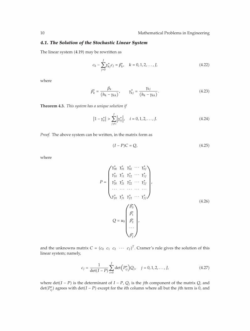
4.1. The Solution of the Stochastic Linear System

The linear system (4.19) may be rewritten as

ck −J∑j=0

γ∗kjcj = β∗k, k = 0, 1, 2, . . . , J, (4.22)

where

β∗k =βk(

hk − γkk) , γ∗kj =

γkj(hk − γkk

) . (4.23)

Theorem 4.3. This system has a unique solution if

∣∣1 − γ∗ii∣∣ >J∑j /= i

∣∣∣γ∗ij∣∣∣, i = 0, 1, 2, . . . , J. (4.24)

Proof. The above system can be written, in the matrix form as

(I − P)C = Q, (4.25)

where

P =

⎛⎜⎜⎜⎜⎜⎜⎜⎜⎝

γ∗00 γ∗01 γ∗02 · · · γ∗0Jγ∗10 γ∗11 γ∗12 · · · γ∗1Jγ∗20 γ∗21 γ∗22 · · · γ∗2J· · · · · · · · · · · · · · ·γ∗J0 γ∗J1 γ∗J2 · · · γ∗JJ

⎞⎟⎟⎟⎟⎟⎟⎟⎟⎠,

Q = u0

⎛⎜⎜⎜⎜⎜⎜⎜⎜⎝

β∗0β∗1β∗2· · ·β∗J

⎞⎟⎟⎟⎟⎟⎟⎟⎟⎠,

(4.26)

and the unknowns matrix C = (c0 c1 c2 · · · cJ)T . Cramer’s rule gives the solution of this

linear system; namely,

cj =1

det(I − P)J∑i=0

det(P ∗ij

)Qj, j = 0, 1, 2, . . . , J, (4.27)

where det(I − P) is the determinant of I − P , Qj is the jth component of the matrix Q, anddet(P ∗

ij) agrees with det(I − P) except for the ith column where all but the jth term is 0, and


the jth term is 1, providing that det(I −P)/= 0; see [12]. It is known that the inverse of the ma-trix I − λP will always exist for all values of λ with the exception of at most J + 1 values.These are the roots of the characteristic determinantal equation det(I−λP) = 0. Therefore, thecondition det(I − P)/= 0 holds if λ = 1 is not an eigenvalue of the matrix P . According toGershgorin theorem, all eigenvalues of the matrix P lie in the circles Si = {z : |z − γ∗ii| ≤∑J

j /= i |γ∗ij |}, i = 0, 1, 2, . . . J . Hence the system (4.22) has a unique solution given by (4.27)if (4.24) is satisfied. As a conclusion of this theorem, our numerical method depends on thechoice of the orthonormal set {ψj(t), j = 0, 1, 2, . . . , J}. This set should be chosen in such a waythat the requirement of the above theorem, (4.24), should be satisfied.

5. Numerical Examples

In this section, we give two examples. The first example is fractional differential equation inwhich there is no stochastic term. The second example is a stochastic differential equation inwhich the differentiation is ordinary not of fractional order.

For each of these examples, we use the Jacobi polynomials of degree k, see [13]

Gk

(p, q, x

)=

Γ(q + k

)Γ(p + 2k

) k∑m=0

(−1)k(k

m

)Γ(p + 2k −m)

Γ(q + k −m) x

k−m,

=k!Γ(p + k

)Γ(p + 2k

) P (p−q,q−1)k (2x − 1), p − q > −1, q > 0

(5.1)

with weight ν(t) = xq−1(1 − x)p−q and satisfy the orthonormality condition

∫1

0ν(x)Gk

(p, q, x

)Gj

(p, q, x

)dx =

⎧⎨⎩hk, k = j,

0, k /= j,(5.2)

where

hk =k!Γ(p + k

)Γ(q + k

)Γ(p − q + k + 1

)(2k + p

)Γ2(p + 2k

) . (5.3)

Example 5.1. Consider the fractional differential equation

CDαu(t) + u(t) = t +Γ(2)

Γ(2 − α) t1−α, u(0) = 0, 0 ≤ t ≤ 1. (5.4)

With exact solution u(t) = t, Table 1 gives the error (error = absolute value of the difference be-tween the exact solution and the approximate solution) for different values of J and Figure 1compares the graph of the exact solution with the graphs of the approximate solutions for


0.2

0.4

0.6

0.8

1

00.2 0.4 0.6 0.8 10

Exact

J = 4

J = 8

J = 2

t

Figure 1: Graph of the error term, Example 5.1, for different values of J .

different values of J = 2, 4, and 8. As an application of this example, the logistic populationgrowth

DβN(t) =r

αN(t)

[1 −

(N(t)K

)α], 0 ≤ β ≤ 1. (5.5)

Example 5.2. Lemma 3.1 shows that the FSIDE (3.2) can be rewritten as (3.6). Therefore, weconsider the stochastic differential equation

du(t) = u(t)dW(t), (5.6)

whose exact solution is

u(t) = u0e(−t/2)+W(t). (5.7)

Denoting by uJ the approximating solution as in (4.17), by u(t) the exact solution, by eJN =max{|u(t) − uJ |, 0 ≤ t ≤ 0.5} the errors, and by αJ = log2e

JN/e

J2N an estimate of a convergence

order, the results are contained in Table 2.


Table 1: The error term, Example 5.1, for different values of J .

t J = 2 J = 4 J = 8

0.01 0.02386082630 0.00739276500 0.001119306570.08 0.0296385222 0.00036210773 0.000423089070.12 0.0239831461 0.0030940054 0.00045735510.18 0.0141698745 0.0042170017 0.00055115020.23 0.0062804608 0.0034445584 0.00001469720.35 0.0088094421 0.0004698618 0.00038131400.46 0.0166034267 0.0028883860 0.00038675470.52 0.0182718028 0.0030401752 0.00039283410.66 0.0151002459 0.0005002161 0.00039807820.73 0.0098778957 0.0014150746 0.00022833390.87 0.0075982376 0.0026085903 0.00029758510.96 0.0236297748 0.0017660564 0.00046625271.00 0.031925763 0.005884759 0.001152260

Table 2: The convergence order, Example 5.2.

N e2N α2 e4N α4 e8N α8

128 0.6240 1.228 5.135 × 10−2 1.5603 8.531 × 10−3 2.913256 0.5103 1.2919 3.291 × 10−2 1.732 2.928 × 10−3 3.321512 0.395 1.5019 1.910 × 10−2 1.873 7.533 × 10−4 3.4511024 0.263 1.014 × 10−2 2.183 × 10−4

6. Conclusion

Our presented numerical method is applied for many different FSIDE of the form (3.2). Fromour numerical computations, we see the following.

(1) There is no restriction on the choice of the orthogonal polynomials. Moreover, thevalues of the parameters, p and q, of the chosen orthogonal polynomials, see (5.1),do not play any role in the computations yet more information about the expectedvalue of the exact solution will be helpful in determining appropriate values ofthese parameters. In all cases the assumed approximation should agree with the in-itial condition with and the exact solution.

(2) If the FSIDE (3.2) is free of the stochastic term while the differentiation is of frac-tional order as in the case of the first example, the method works quite well.

(3) In case of the existence of the stochastic term, as in the case of the second example,although the method is of higher-order accuracy yet in practice the obtained resultsare not quite well as with the previous case.

(4) We note that for every path, even with a series of Monte Carlo simulations, the sto-chastic linear system, (4.22), yields a unique deterministic solution.


Acknowledgment

The authors would like to thank Professor Bill Mclean for his valuable discussions regardingthis work.

References

[1] T. M. Atanackovic and B. Stankovic, “On a system of differential equations with fractional derivativesarising in rod theory,” Journal of Physics A, vol. 37, no. 4, pp. 1241–1250, 2004.

[2] A. A. Kilbas, H. M. Srivastava, and J. J. Trujillo, Theory and Applications of Fractional Differential Equa-tions, vol. 204 of North-Holland Mathematics Studies, Elsevier, Amsterdam, The Netherlands, 2006.

[3] R. L. Magin, “Fractional calculus in bioengineering,” Critical Reviews in Biomedical Engineering, vol. 32,no. 1, pp. 1–104, 2004.

[4] R. L. Magin, “Fractional calculus in bioengineering, part 2,” Critical Reviews in Biomedical Engineering,vol. 32, no. 2, pp. 105–193, 2004.

[5] R. L. Magin, “Fractional calculus in bioengineering, part 3,” Critical Reviews in Biomedical Engineering,vol. 32, no. 3-4, pp. 195–377, 2004.

[6] B. Bouchard and N. Touzi, “Discrete-time approximation and Monte-Carlo simulation of backwardstochastic differential equations,” Stochastic Processes and their Applications, vol. 111, no. 2, pp. 175–206,2004.

[7] F.-R. Chang, Stochastic Optimization in Continuous Time, Cambridge University Press, Cambridge, UK,2004.

[8] X. Mao, “Numerical solutions of stochastic functional differential equations,” LMS Journal of Comput-ation and Mathematics, vol. 6, pp. 141–161, 2003.

[9] S. I. Denisov, P. Hanggi, and H. Kantz, “Parameters of the fractional Fokker-Planck equation,” EPL,vol. 85, no. 4, Article ID 40007, 2009.

[10] P. E. Kloeden and E. Platen,Numerical Solution of Stochastic Differential Equations, vol. 23 of Applicationsof Mathematics, Springer, Berlin, Germany, 1992.

[11] E. J. Allen, S. J. Novosel, and Z. Zhang, “Finite element and difference approximation of some linearstochastic partial differential equations,” Stochastics and Stochastics Reports, vol. 64, no. 1-2, pp. 117–142, 1998.

[12] H. Hochstadt, Integral Equations, Pure and Applied Mathematics, John Wiley & Sons, London, UK,1973.

[13] M. Abramowitz and I. A. Stegun, Eds., Handbook of Mathematical Functions, with Formulas, Graphs, andMathematical Tables, Dover, New York, NY, USA, 1966.

Submit your manuscripts athttp://www.hindawi.com

Hindawi Publishing Corporationhttp://www.hindawi.com Volume 2014

MathematicsJournal of


Mathematical Problems in Engineering

Hindawi Publishing Corporationhttp://www.hindawi.com

Differential EquationsInternational Journal of

Volume 2014

Applied MathematicsJournal of


Probability and StatisticsHindawi Publishing Corporationhttp://www.hindawi.com Volume 2014

Journal of


Mathematical PhysicsAdvances in

Complex AnalysisJournal of


OptimizationJournal of


CombinatoricsHindawi Publishing Corporationhttp://www.hindawi.com Volume 2014

International Journal of


Operations ResearchAdvances in

Journal of


Function Spaces

Abstract and Applied AnalysisHindawi Publishing Corporationhttp://www.hindawi.com Volume 2014

International Journal of Mathematics and Mathematical Sciences


The Scientific World JournalHindawi Publishing Corporation http://www.hindawi.com Volume 2014


Algebra

Discrete Dynamics in Nature and Society



Decision SciencesAdvances in

Discrete MathematicsJournal of

Hindawi Publishing Corporationhttp://www.hindawi.com

Volume 2014 Hindawi Publishing Corporationhttp://www.hindawi.com Volume 2014

Stochastic AnalysisInternational Journal of

Documents

Monte-Carlo Galerkin Approximation of Fractional ...downloads.hindawi.com/journals/mpe/2012/709106.pdfAbdallah Ali Badr1 and Hanan Salem El-Hoety2 1 Department of Mathematics, Faculty