Embed Size (px)
Citation preview
Monte Carlo methods for the approximation andmitigation of rare events, II
Paul Dupuis
Division of Applied MathematicsBrown University
Probability and Simulation (Recent Trends)
Centre Henri LebesgueRennes
June 2018
Outline
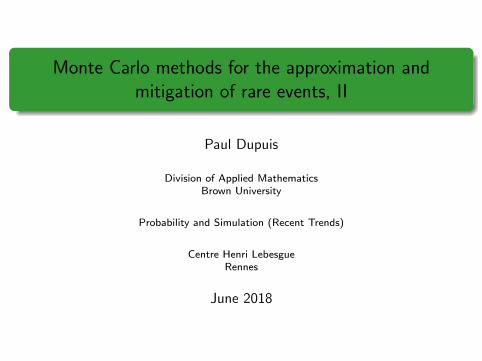
Introduction
Examples (counting, UQ, chemistry) illustrating rare event samplingproblemModels (jump for discrete state, di�usion or Markov chain forcontinuous)
Parallel tempering/replica exchange
Formulation in discrete timeFormulation in continuous timePerformance criteria
Optimization with respect to swap rate
Form of the rate functionThe in�nite swapping limit{symmetrized dynamics and a weightedempirical measureAsymptotic varianceImplementation issues and partial in�nite swappingExamples
Outline
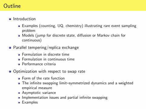
Other uses of the large deviation rate function
A one sided convergence diagnosticHow poor numerical approximations are most likely to occur
Optimization with respect to temperature placement{low temperaturelimit
Sources of variance reductionA simpli�ed model{in�nite swapping with IID samplesLow temperature limit via Freidlin-Wentsell methodsOptimal temperatures in the low temperature limit
Summary
Some problems of interest
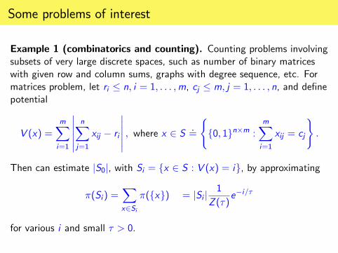
Example 1 (combinatorics and counting). Counting problems involvingsubsets of very large discrete spaces, such as number of binary matriceswith given row and column sums, graphs with degree sequence, etc. Formatrices problem, let ri � n; i = 1; : : : ;m, cj � m; j = 1; : : : ; n, and de�nepotential
V (x) =mXi=1
������nXj=1
xij � ri
������ ; where x 2 S :=
(f0; 1gn�m :
mXi=1
xij = cj
):
Then can estimate jS0j, with Si = fx 2 S : V (x) = ig, by approximating
�(Si ) =Xx2Si
�(fxg) = jSi j1
Z (�)e�i=�
for various i and small � > 0.
Some problems of interest
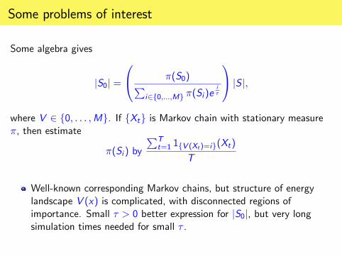
Some algebra gives
jS0j =
0@ �(S0)Pi2f0;:::;Mg �(Si )e
i�
1A jS j;where V 2 f0; : : : ;Mg. If fXtg is Markov chain with stationary measure�, then estimate
�(Si ) by
PTt=1 1fV (Xt)=ig(Xt)
T
Well-known corresponding Markov chains, but structure of energylandscape V (x) is complicated, with disconnected regions ofimportance. Small � > 0 better expression for jS0j, but very longsimulation times needed for small � .
Some problems of interest
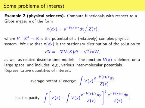
Example 2 (physical sciences). Compute functionals with respect to aGibbs measure of the form
�(dx) = e�V (x)=�dx.Z (�);
where V : Rd ! R is the potential of a (relatively) complex physicalsystem. We use that �(dx) is the stationary distribution of the solution to
dX = �rV (X )dt +p2�dW ;
as well as related discrete time models. The function V (x) is de�ned on alarge space, and includes, e.g., various inter-molecular potentials.Representative quantities of interest:
average potential energy:
ZV (x)
e�V (x)=�dx
Z (�)
heat capacity:
Z "V (x)�
ZV (y)
e�V (y)=�dy
Z (�)
#2e�V (x)=�dx
Z (�):
Some problems of interest
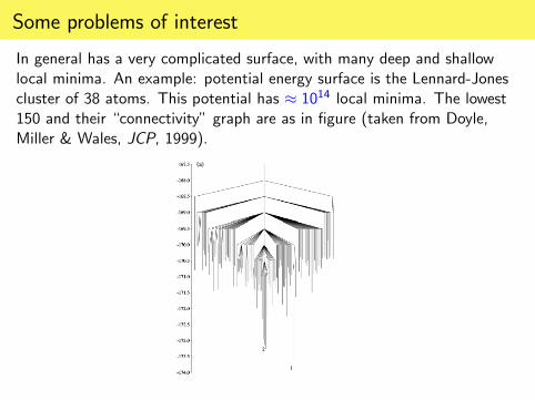
In general has a very complicated surface, with many deep and shallowlocal minima. An example: potential energy surface is the Lennard-Jonescluster of 38 atoms. This potential has � 1014 local minima. The lowest150 and their \connectivity" graph are as in �gure (taken from Doyle,Miller & Wales, JCP, 1999).
Some problems of interest
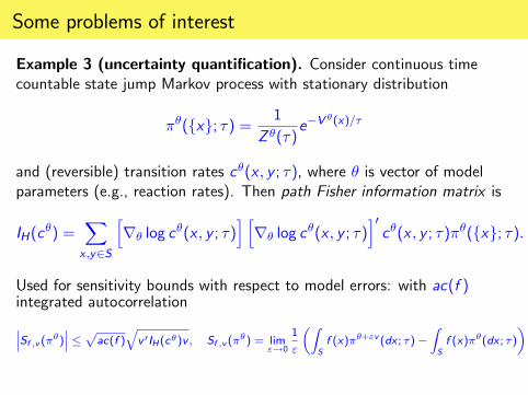
Example 3 (uncertainty quanti�cation). Consider continuous timecountable state jump Markov process with stationary distribution
��(fxg; �) = 1
Z �(�)e�V
�(x)=�
and (reversible) transition rates c�(x ; y ; �), where � is vector of modelparameters (e.g., reaction rates). Then path Fisher information matrix is
IH(c�) =
Xx ;y2S
hr� log c�(x ; y ; �)
i hr� log c�(x ; y ; �)
i0c�(x ; y ; �)��(fxg; �):
Used for sensitivity bounds with respect to model errors: with ac(f )integrated autocorrelation
���Sf ;v (��)��� �pac(f )qv 0IH(c�)v ; Sf ;v (��) = lim
"!0
1
"
�ZSf (x)��+"v (dx ; �)�
ZSf (x)��(dx ; �)
�:
Process models
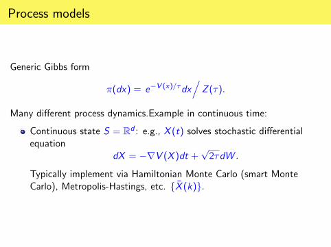
Generic Gibbs form
�(dx) = e�V (x)=�dx.Z (�):
Many di�erent process dynamics.Example in continuous time:
Continuous state S = Rd : e.g., X (t) solves stochastic di�erentialequation
dX = �rV (X )dt +p2�dW :
Typically implement via Hamiltonian Monte Carlo (smart MonteCarlo), Metropolis-Hastings, etc. f �X (k)g.
Process models
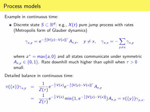
Example in continuous time:
Discrete state S � Rd : e.g., X (t) pure jump process with rates(Metropolis form of Glauber dynamics)
x ;y = e� 1�[V (y)�V (x)]+Ax ;y ; y 6= x ; x ;x = �
Xy 6=x
x ;y
where a+ = maxfa; 0g and all states communicate under symmetricAx ;y 2 f0; 1g. Rate downhill much higher than uphill when � > 0small.
Detailed balance in continuous time:
�(fxg) x ;y =1
Z (�)e�
1�V (x)e�
1�[V (y)�V (x)]+Ax ;y
=1
Z (�)e�
1�V (x)minf1; e�
1�[V (y)�V (x)]gAx ;y = �(fyg) y ;x :
Process models
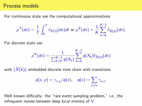
For continuous state use the computational approximations
�T (dx) =1
T
Z T
0�X (t)(dx)dt or �
K (dx) =1
K
K�1Xk=0
� �X (k)(dx):
For discrete state use
�K (dx) =1PK�1
k=0 q(Xk)
K�1Xk=0
q(Xk)� �X (k)(dx)
with f �X (k)g embedded discrete time chain with transitions
p(x ; y) = x ;y=q(x); q(x) =Xy 6=x
x ;y :
Well known di�culty: the \rare event sampling problem," i.e., theinfrequent moves between deep local minima of V .
Parallel tempering for di�usion
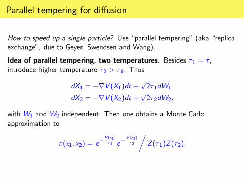
How to speed up a single particle? Use \parallel tempering" (aka \replicaexchange", due to Geyer, Swendsen and Wang).
Idea of parallel tempering, two temperatures. Besides �1 = � ,introduce higher temperature �2 > �1. Thus
dX1 = �rV (X1)dt +p2�1dW1
dX2 = �rV (X2)dt +p2�2dW2;
with W1 and W2 independent. Then one obtains a Monte Carloapproximation to
�(x1; x2) = e�V (x1)
�1 e�V (x2)
�2
�Z (�1)Z (�2):
Parallel tempering for di�usion
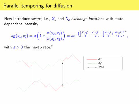
Now introduce swaps, i.e., X1 and X2 exchange locations with statedependent intensity
ag(x1; x2) = a
�1 ^ �(x2; x1)
�(x1; x2)
�= ae
��h
V (x2)�1
+V (x1)�2
i�hV (x1)�1
+V (x2)�2
i�+;
with a > 0 the \swap rate."
Parallel tempering for di�usion
Now have a Markov jump-di�usion. Easy to check: since Glauber(Metropolis) jump rate used still have detailed balance, and thus
�a(x1; x2) = �(x1; x2) = e�V (x1)
�1 e�V (x2)
�2
�Z (�1)Z (�2):
Higher temperature �2 > �1 � greater di�usivity of X a2
� easier communication for X a2
� passed to X a1 via swaps
This helps overcome the \rare event sampling problem."
Parallel tempering for pure jump
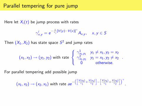
Here let Xi (t) be jump process with rates
ix ;y = e� 1� i[V (y)�V (x)]+
Ax ;y ; x ; y 2 S
Then (X1;X2) has state space S2 and jump rates
(x1; x2)! (y1; y2) with rate
8<: 1x1;y1 y1 6= x1; y2 = x2 2x2;y2 y1 = x1; y2 6= x20 otherwise.
:
For parallel tempering add possible jump
(x1; x2)! (x2; x1) with rate ae��h
V (x2)�1
+V (x1)�2
i�hV (x1)�1
+V (x2)�2
i�+:
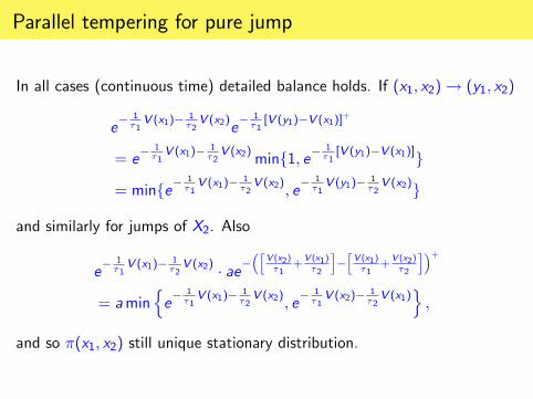
Parallel tempering for pure jump
In all cases (continuous time) detailed balance holds. If (x1; x2)! (y1; x2)
e� 1�1V (x1)� 1
�2V (x2)e
� 1�1[V (y1)�V (x1)]+
= e� 1�1V (x1)� 1
�2V (x2)minf1; e�
1�1[V (y1)�V (x1)]g
= minfe�1�1V (x1)� 1
�2V (x2); e
� 1�1V (y1)� 1
�2V (x2)g
and similarly for jumps of X2. Also
e� 1�1V (x1)� 1
�2V (x2) � ae�
�hV (x2)�1
+V (x1)�2
i�hV (x1)�1
+V (x2)�2
i�+= amin
ne� 1�1V (x1)� 1
�2V (x2); e
� 1�1V (x2)� 1
�2V (x1)
o;
and so �(x1; x2) still unique stationary distribution.
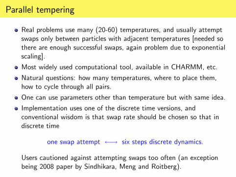
Parallel tempering
Real problems use many (20-60) temperatures, and usually attemptswaps only between particles with adjacent temperatures [needed sothere are enough successful swaps, again problem due to exponentialscaling].
Most widely used computational tool, available in CHARMM, etc.
Natural questions: how many temperatures, where to place them,how to cycle through all pairs.
One can use parameters other than temperature but with same idea.
Implementation uses one of the discrete time versions, andconventional wisdom is that swap rate should be chosen so that indiscrete time
one swap attempt ! six steps discrete dynamics.
Users cautioned against attempting swaps too often (an exceptionbeing 2008 paper by Sindhikara, Meng and Roitberg).
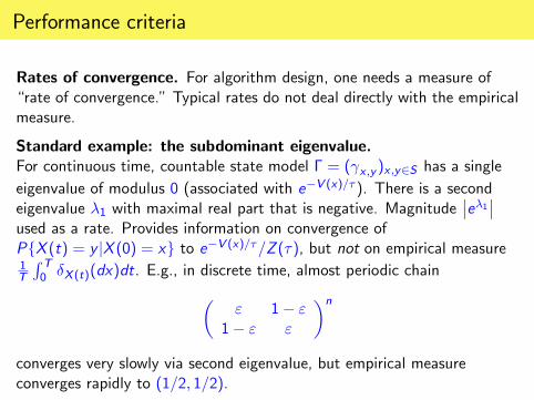
Performance criteria
Rates of convergence. For algorithm design, one needs a measure of\rate of convergence." Typical rates do not deal directly with the empiricalmeasure.
Standard example: the subdominant eigenvalue.For continuous time, countable state model � = ( x ;y )x ;y2S has a single
eigenvalue of modulus 0 (associated with e�V (x)=� ). There is a secondeigenvalue �1 with maximal real part that is negative. Magnitude
��e�1��used as a rate. Provides information on convergence ofPfX (t) = y jX (0) = xg to e�V (x)=�=Z (�), but not on empirical measure1T
R T0 �X (t)(dx)dt. E.g., in discrete time, almost periodic chain�
" 1� "1� " "
�nconverges very slowly via second eigenvalue, but empirical measureconverges rapidly to (1=2; 1=2).
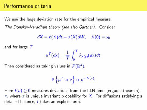
Performance criteria
We use the large deviation rate for the empirical measure.
The Donsker-Varadhan theory (see also G�artner). Consider
dX = b(X )dt + �(X )dW ; X (0) = x0
and for large T
�T (dx) =1
T
Z T
0�X (t)(dx)dt:
Then considered as taking values in P(Rd),
Pn�T � �
o� e�TI (�):
Here I (�) � 0 measures deviations from the LLN limit (ergodic theorem)�, where � is unique invariant probability for X . For di�usions satisfying adetailed balance, I takes an explicit form.
Performance criteria
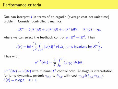
One can interpret I in terms of an ergodic (average cost per unit time)problem. Consider controlled dynamics
dX u = b(X u)dt + u(X u)dt + �(X u)dW ; X u(0) = x0;
where we can select the feedback control u : Rd ! Rd . Then
I (�) = inf
�1
2
ZRdku(x)k2 �(dx) : � is invariant for X u
�:
Thus with
�u;T (dx) =1
T
Z T
0�X u(t)(dx)dt;
�u;T (dx)! �(dx) with minimal L2 control cost. Analogous intepretationfor jump dynamics, perturb x ;y to � x ;y with cost x ;y `(� x ;y= x ;y ),` (z) = z log z � z + 1.
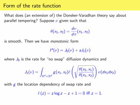
Form of the rate function
What does (an extension of) the Donsker-Varadhan theory say aboutparallel tempering? Suppose � given such that
�(x1; x2) =d�
d�(x1; x2)
is smooth. Then we have monotonic form
I a(�) = J0(�) + aJ1(�)
where J0 is the rate for \no swap" di�usion dynamics and
J1(�) =
ZRd�Rd
g(x1; x2)`
s�(x2; x1)
�(x1; x2)
!�(dx1dx2)
with g the location dependency of swap rate and
` (z) = z log z � z + 1 = 0 i� z = 1:
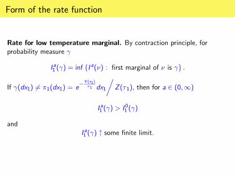
Form of the rate function
Rate for low temperature marginal. By contraction principle, forprobability measure
I a1 ( ) = inf fI a(�) : �rst marginal of � is g :
If (dx1) 6= �1(dx1) = e�V (x1)
�1 dx1
�Z (�1), then for a 2 (0;1)
I a1 ( ) > I01 ( )
andI a1 ( ) " some �nite limit.
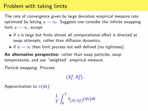
Problem with taking limits
The rate of convergence given by large deviation empirical measure rateoptimized by letting a!1. Suggests one consider the in�nite swappinglimit a!1, except
if a is large but �nite almost all computational e�ort is directed atswap attempts, rather than di�usion dynamics,
if a!1 then limit process not well de�ned (no tightness).
An alternative perspective: rather than swap particles, swaptemperatures, and use \weighted" empirical measure.
Particle swapping. Process:
(X a1 ;Xa2 ) ;
Approximation to �(dx):
1
T
Z T
0�(X a1 ;X a2 )
(dx)dt
The in�nite swapping limit
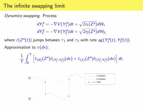
Dynamics swapping. Process:
dY a1 = �rV (Y a1 )dt +p2r1(Z a)dW1
dY a2 = �rV (Y a2 )dt +p2r2(Z a)dW2;
where r(Z a(t)) jumps between �1 and �2 with rate ag(Ya1 (t);Y
a2 (t)).
Approximation to �(dx):
1
T
Z T
0
h1f0g(Z
a)�(Y a1 ;Y a2 )(dx) + 1f1g(Za)�(Y a2 ;Y a1 )(dx)
idt:
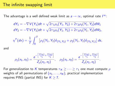
The in�nite swapping limit
The advantage is a well de�ned weak limit as a!1, optimal rate I1:
dY1 = �rV (Y1)dt +p2�1�1(Y1;Y2) + 2�2�2(Y1;Y2)dW1
dY2 = �rV (Y2)dt +p2�2�1(Y1;Y2) + 2�1�2(Y1;Y2)dW2;
�T (dx) =1
T
Z T
0
��1(Y1;Y2)�(Y1;Y2) + �2(Y1;Y2)�(Y2;Y1)
�ds;
and
�1(x1; x2) =e�hV (x1)�1
+V (x2)�2
iZ�(x1; x2)
; �2(x1; x2) =e�hV (x2)�1
+V (x1)�2
iZ�(x1; x2)
:
For generalization to K temperatures �K � � � � � �1 one must compute �weights of all permutations of (x1; : : : ; xK ), practical implementationrequires PINS (partial INS) for K � 7.
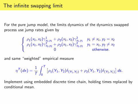
The in�nite swapping limit
For the pure jump model, the limits dynamics of the dynamics swappedprocess use jump rates given by8<:
�1(x1; x2) 1x1;y1 + �2(x1; x2)
2x1;y1 y1 6= x1; y2 = x2
�1(x1; x2) 2x2;y2 + �2(x1; x2)
2x2;y2 y1 = x1; y2 6= x2
0 otherwise.
and same \weighted" empirical measure
�T (dx) =1
T
Z T
0
��1(Y1;Y2)�(Y1;Y2) + �2(Y1;Y2)�(Y2;Y1)
�ds:
Implement using embedded discrete time chain, holding times replaced byconditional mean.
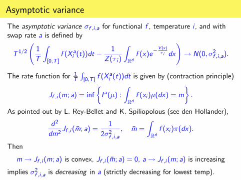
Asymptotic variance
The asymptotic variance �f ;i ;a for functional f , temperature i , and withswap rate a is de�ned by
T 1=2
1
T
Z[0;T ]
f (X ai (t))dt �1
Z (� i )
ZRdf (x)e
�V (x)� i dx
!! N(0; �2f ;i ;a):
The rate function for 1T
R[0;T ] f (X
ai (t))dt is given by (contraction principle)
Jf ;i (m; a) = inf
�I a(�) :
ZRdf (xi )�(dx) = m
�:
As pointed out by L. Rey-Bellet and K. Spiliopolous (see den Hollander),
d2
dm2Jf ;i ( �m; a) =
1
2�2f ;i ;a; �m =
ZRdf (xi )�(dx):
Then
m! Jf ;i (m; a) is convex, Jf ;i ( �m; a) = 0, a! Jf ;i (m; a) is increasing
implies �2f ;i ;a is decreasing in a (strictly decreasing for lowest temp).
Implementation issues and partial in�nite swapping
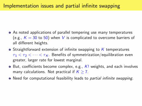
As noted applications of parallel tempering use many temperatures(e.g., K = 30 to 50) when V is complicated to overcome barriers ofall di�erent heights.
Straightforward extension of in�nite swapping to K temperatures�1 < �2 < � � � < �K . Bene�ts of symmetrization/equilibration evengreater, larger rate for lowest marginal.
But, coe�cients become complex, e.g., K ! weights, and each involvesmany calculations. Not practical if K � 7.Need for computational feasibility leads to partial in�nite swapping.
Implementation issues and partial in�nite swapping
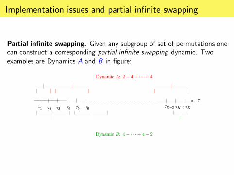
Partial in�nite swapping. Given any subgroup of set of permutations onecan construct a corresponding partial in�nite swapping dynamic. Twoexamples are Dynamics A and B in �gure:
Implementation issues and partial in�nite swapping
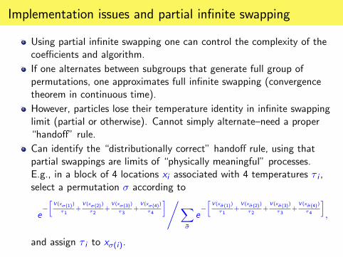
Using partial in�nite swapping one can control the complexity of thecoe�cients and algorithm.
If one alternates between subgroups that generate full group ofpermutations, one approximates full in�nite swapping (convergencetheorem in continuous time).
However, particles lose their temperature identity in in�nite swappinglimit (partial or otherwise). Cannot simply alternate{need a proper\hando�" rule.
Can identify the \distributionally correct" hando� rule, using thatpartial swappings are limits of \physically meaningful" processes.E.g., in a block of 4 locations xi associated with 4 temperatures � i ,select a permutation � according to
e��V (x�(1))
�1+V (x�(2))
�2+V (x�(3))
�3+V (x�(4))
�4
�,X��
e��V (x ��(1))
�1+V (x ��(2))
�2+V (x ��(3))
�3+V (x ��(4))
�4
�;
and assign � i to x�(i).
Examples
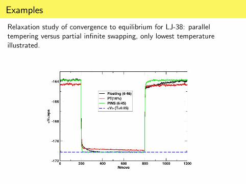
Relaxation study of convergence to equilibrium for LJ-38.
quantity of interest: average potential energy at various temperatures
used 45 temperatures, 3{6{6{� � � {6 type dynamic for partial in�niteswapping
used Smart Monte Carlo for particle dynamics
lowest 1/3 of temperatures raised to push process away fromequilibrium (low temperature components pushed away from deepminima)
then reduced to correct temperatures for 600 discrete time steps tostudy return to equilibria
repeated 2000 times, we plot averages for lowest (and hardest)temperature
Examples
Relaxation study of convergence to equilibrium for LJ-38: paralleltempering versus partial in�nite swapping, only lowest temperatureillustrated.
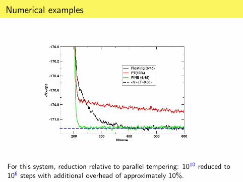
Numerical examples
For this system, reduction relative to parallel tempering: 1010 reduced to106 steps with additional overhead of approximately 10%.
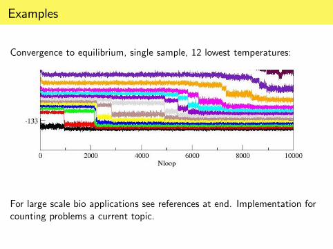
Examples
Convergence to equilibrium, single sample, 12 lowest temperatures:
For large scale bio applications see references at end. Implementation forcounting problems a current topic.
Other uses of the large deviation rate function
The rate function in principle captures many other interesting properties ofwhatever MC scheme is being used. Di�culty is extracting information.Examples:
Necessary conditions for convergence
Where good/bad sampling of transitions has greatest impact onoverall quality of approximation
Optimal placement of temperatures for particular functionals
Sources of variance reduction
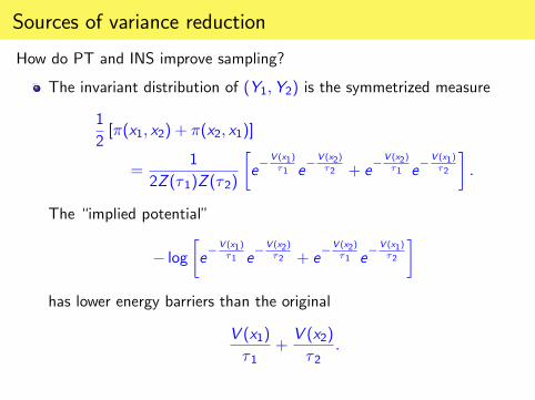
How do PT and INS improve sampling?
The invariant distribution of (Y1;Y2) is the symmetrized measure
1
2[�(x1; x2) + �(x2; x1)]
=1
2Z (�1)Z (�2)
�e�V (x1)
�1 e�V (x2)
�2 + e�V (x2)
�1 e�V (x1)
�2
�:
The \implied potential"
� log�e�V (x1)
�1 e�V (x2)
�2 + e�V (x2)
�1 e�V (x1)
�2
�has lower energy barriers than the original
V (x1)
�1+V (x2)
�2:
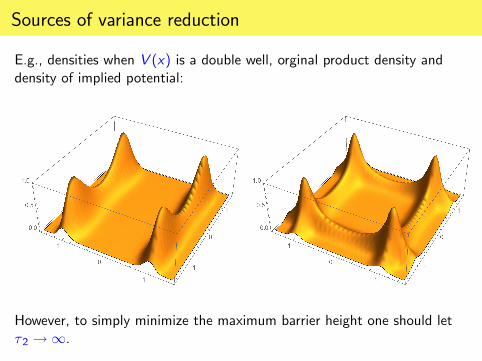
Sources of variance reduction
E.g., densities when V (x) is a double well, orginal product density anddensity of implied potential:
However, to simply minimize the maximum barrier height one should let�2 !1.
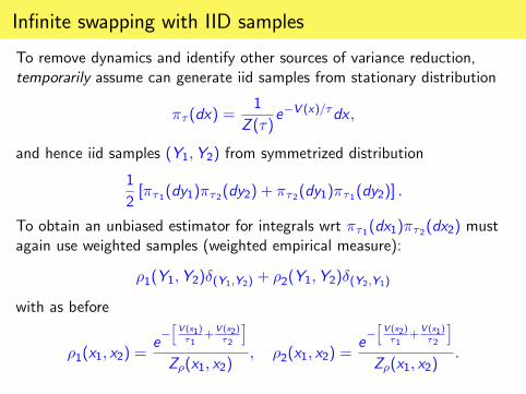
In�nite swapping with IID samples
To remove dynamics and identify other sources of variance reduction,temporarily assume can generate iid samples from stationary distribution
�� (dx) =1
Z (�)e�V (x)=�dx ;
and hence iid samples (Y1;Y2) from symmetrized distribution
1
2[��1(dy1)��2(dy2) + ��2(dy1)��1(dy2)] :
To obtain an unbiased estimator for integrals wrt ��1(dx1)��2(dx2) mustagain use weighted samples (weighted empirical measure):
�1(Y1;Y2)�(Y1;Y2) + �2(Y1;Y2)�(Y2;Y1)
with as before
�1(x1; x2) =e�hV (x1)�1
+V (x2)�2
iZ�(x1; x2)
; �2(x1; x2) =e�hV (x2)�1
+V (x1)�2
iZ�(x1; x2)
:
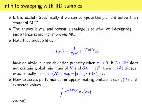
In�nite swapping with IID samples
Is this useful? Speci�cally, if we can compute the �'s, is it better thanstandard MC?
The answer is yes, and reason is analogous to why (well designed)importance sampling improves MC.
Note that probabilities
�� (dx) =1
Z (�)e�V (x)=�dx
have an obvious large deviation property when � ! 0. If A � Rd doesnot contain global minimum of V and @A \nice", then �� (A) decaysexponentially in � : �� (A) � exp� [infx2A V (x)] =� .How to assess performance for approximating probabilities �� (A) andexpected values Z
e�1�F (x)�� (dx)
via MC?
In�nite swapping with IID samples
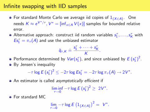
For standard Monte Carlo we average iid copies of 1fX2Ag. One
needs K � eV �=� ;V � = [infx2A V (x)] samples for bounded relativeerror.Alternative approach: construct iid random variables s�1 ; : : : ; s
�K with
Es�1 = �� (A) and use the unbiased estimator
q̂�;K:=s�1 + � � �+ s�K
K:
Performance determined by Var(s�1 ), and since unbiased by E (s�1 )2.
By Jensen's inequality
�� log E (s�1 )2 � �2� log Es�1 = �2� log �� (A)! 2V �:
An estimator is called asymptotically e�cient if
lim inf�!0
�� log E (s�1 )2 � 2V �:
For standard MC
lim�!0�� log E
�1fX2Ag
�2= V �:
In�nite swapping with IID samples
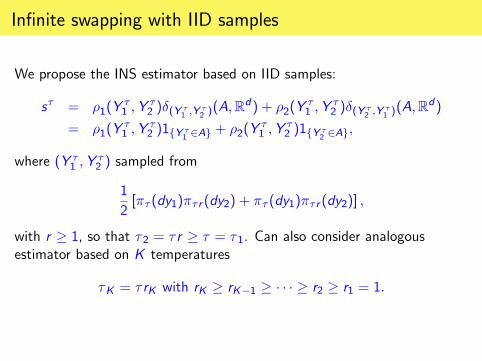
We propose the INS estimator based on IID samples:
s� = �1(Y�1 ;Y
�2 )�(Y �1 ;Y �2 )(A;R
d) + �2(Y�1 ;Y
�2 )�(Y �2 ;Y �1 )(A;R
d)
= �1(Y�1 ;Y
�2 )1fY �1 2Ag + �2(Y
�1 ;Y
�2 )1fY �2 2Ag;
where (Y �1 ;Y�2 ) sampled from
1
2[�� (dy1)�� r (dy2) + �� (dy1)�� r (dy2)] ;
with r � 1, so that �2 = � r � � = �1. Can also consider analogousestimator based on K temperatures
�K = � rK with rK � rK�1 � � � � � r2 � r1 = 1:
In�nite swapping with IID samples
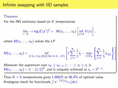
Theorem
For the INS estimator based on K temperatures
lim�!0�� log E (s� )2 = M(r1; : : : ; rK )
�infx2A
V (x)
�;
where M(r1; : : : ; rK ) solves the LP
M(r1; : : : ; rK ) = inffI :I1=1;Ik2[0;1] for k=2;:::;Kg
242 KXj=1
1
rjIj � min
�2�K
8<:KXj=1
1
rjI�(j)
9=;35 :
Moreover the supremum over rK � rK�1 � � � � � r2 � r1 isM(r1; : : : ; rK ) = 2� (1=2)K and is uniquely achieved at rk = 2k�1.
Thus K = 5 temperatures gives 1:96875 or 98:4% of optimal value.
Analogous result for functionalsRe�
1�F (x)�� (dx).
In�nite swapping with IID samples
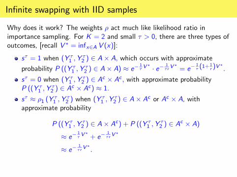
Why does it work? The weights � act much like likelihood ratio inimportance sampling. For K = 2 and small � > 0, there are three types ofoutcomes, [recall V � = infx2A V (x)]:
s� = 1 when (Y �1 ;Y�2 ) 2 A� A; which occurs with approximate
probability P ((Y �1 ;Y�2 ) 2 A� A) � e�
1�V � � e� 1
� rV � = e�
1� (1+
1r )V
�.
s� = 0 when (Y �1 ;Y�2 ) 2 Ac � Ac ; with approximate probability
P ((Y �1 ;Y�2 ) 2 Ac � Ac) � 1.
s� � �1 (Y �1 ;Y �2 ) when (Y �1 ;Y �2 ) 2 A� Ac or Ac � A, withapproximate probability
P ((Y �1 ;Y�2 ) 2 A� Ac) + P ((Y �1 ;Y �2 ) 2 Ac � A)
� e�1�V � + e�
1� rV �
� e�1� rV � :
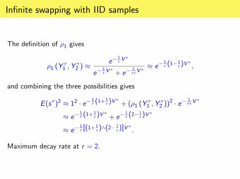
In�nite swapping with IID samples
The de�nition of �1 gives
�1 (Y�1 ;Y
�2 ) �
e�1�V �
e�1�V � + e�
1� rV �� e�
1� (1�
1r )V
�;
and combining the three possibilities gives
E (s� )2 � 12 � e�1� (1+
1r )V
�+ (�1 (Y
�1 ;Y
�2 ))
2 � e�1� rV �
� e�1� (1+
1r )V
�+ e�
1� (2�
1r )V
�
� e�1� [(1+
1r )^(2�
1r )]V
�:
Maximum decay rate at r = 2.
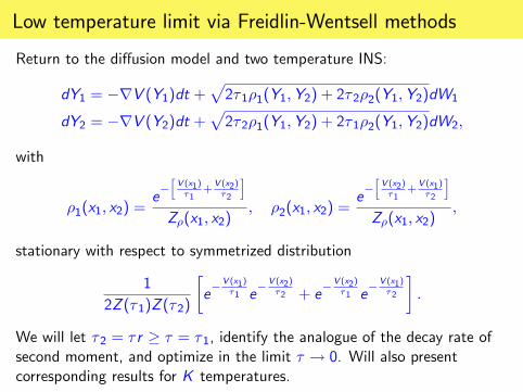
Low temperature limit via Freidlin-Wentsell methods
Return to the di�usion model and two temperature INS:
dY1 = �rV (Y1)dt +p2�1�1(Y1;Y2) + 2�2�2(Y1;Y2)dW1
dY2 = �rV (Y2)dt +p2�2�1(Y1;Y2) + 2�1�2(Y1;Y2)dW2;
with
�1(x1; x2) =e�hV (x1)�1
+V (x2)�2
iZ�(x1; x2)
; �2(x1; x2) =e�hV (x2)�1
+V (x1)�2
iZ�(x1; x2)
;
stationary with respect to symmetrized distribution
1
2Z (�1)Z (�2)
�e�V (x1)
�1 e�V (x2)
�2 + e�V (x2)
�1 e�V (x1)
�2
�:
We will let �2 = � r � � = �1, identify the analogue of the decay rate ofsecond moment, and optimize in the limit � ! 0. Will also presentcorresponding results for K temperatures.
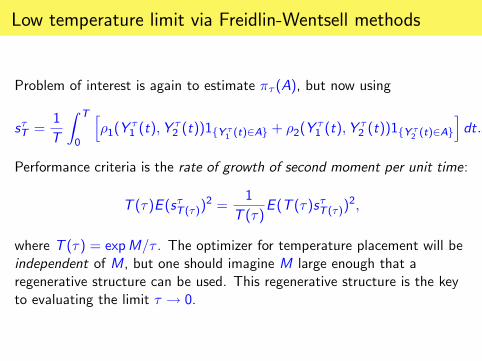
Low temperature limit via Freidlin-Wentsell methods
Problem of interest is again to estimate �� (A), but now using
s�T =1
T
Z T
0
h�1(Y
�1 (t);Y
�2 (t))1fY �1 (t)2Ag + �2(Y
�1 (t);Y
�2 (t))1fY �2 (t)2Ag
idt:
Performance criteria is the rate of growth of second moment per unit time:
T (�)E (s�T (�))2 =
1
T (�)E (T (�)s�T (�))
2;
where T (�) = expM=� . The optimizer for temperature placement will beindependent of M, but one should imagine M large enough that aregenerative structure can be used. This regenerative structure is the keyto evaluating the limit � ! 0.
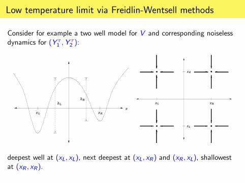
Low temperature limit via Freidlin-Wentsell methods
Consider for example a two well model for V and corresponding noiselessdynamics for (Y �1 ;Y
�2 ):
deepest well at (xL; xL), next deepest at (xL; xR) and (xR ; xL), shallowestat (xR ; xR).
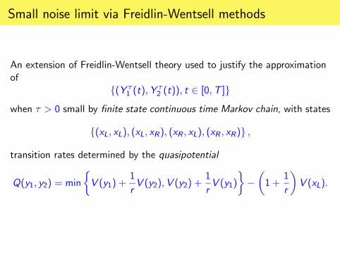
Small noise limit via Freidlin-Wentsell methods
An extension of Freidlin-Wentsell theory used to justify the approximationof
f(Y �1 (t);Y �2 (t)); t 2 [0;T ]g
when � > 0 small by �nite state continuous time Markov chain, with states
f(xL; xL); (xL; xR); (xR ; xL); (xR ; xR)g ;
transition rates determined by the quasipotential
Q(y1; y2) = min
�V (y1) +
1
rV (y2);V (y2) +
1
rV (y1)
���1 +
1
r
�V (xL):
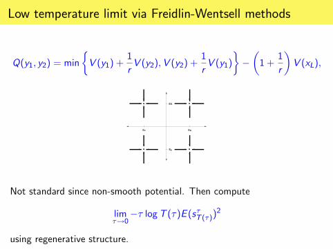
Low temperature limit via Freidlin-Wentsell methods
Q(y1; y2) = min
�V (y1) +
1
rV (y2);V (y2) +
1
rV (y1)
���1 +
1
r
�V (xL);
Not standard since non-smooth potential. Then compute
lim�!0�� logT (�)E (s�T (�))
2
using regenerative structure.
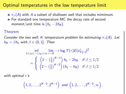
Optimal temperatures in the low temperature limit
�� (A) with A a subset of shallower well that includes mimimum.For standard one temperature MC the decay rate of secondmoment/unit time is (hL � 2hR).
Theorem
Consider the two well, K temperature problem for estimating �� (A). LethR = �hL with � 2 (0; 1]. Then
inf1�r2�����rK�1
lim�!0�� logT (�)E (s�T (�))
2
=
8<:�2�
�12
�K�1�hL � 2hR if � � 1=2�
2��12
�K�2�(hL � hR) if � � 1=2
with optimal r 's�1; 2; : : : ; 2K�2; 2K�1
�and
�1; 2; : : : ; 2K�2;1
�:
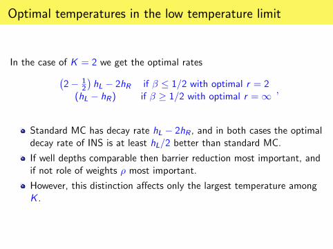
Optimal temperatures in the low temperature limit
In the case of K = 2 we get the optimal rates�2� 1
2
�hL � 2hR if � � 1=2 with optimal r = 2
(hL � hR) if � � 1=2 with optimal r =1 ;
Standard MC has decay rate hL � 2hR , and in both cases the optimaldecay rate of INS is at least hL=2 better than standard MC.
If well depths comparable then barrier reduction most important, andif not role of weights � most important.
However, this distinction a�ects only the largest temperature amongK .
Optimal temperatures in the low temperature limit
Generalizations/comments:
All cases of three well model have optimal temperatures in small noiselimit as one of these two forms
Conjecture that same is true for arbitrary �nite number of wells
Analogous results for functionals, discrete time models
Geometric spacing has been suggested based on other arguments forPT/INS (see references)

Summary
\Rare events" issues of various sorts are one of the banes of e�cientMonte Carlo
As such, it is natural to use various asymptotic theories to understandissues of algorithm design
There is a relatively long history of the use of large deviation ideas inthe design of algorithms for estimating probabilities of single rareevents, but less on how to overcome impact of rare events on MCMC
Have presented two such uses in the context of parallel replicaalgorithms to optimize and understand understand the mechanismsthat produce variance reduction
References
Parallel tempering:
\Replica Monte Carlo simulation of spin glasses", Swendsen andWang, Phys. Rev. Lett., 57, 2607{2609, 1986.
\Markov chain Monte Carlo maximum likelihood", Geyer inComputing Science and Statistics: Proceedings of the 23rdSymposium on the Interface, ASA, 156{163, 1991.
A paper suggesting it is good to swap a lot:
\Exchange frequency in replica exchange molecular dynamics",Sindhikara, Meng and Roitberg, J. of Chem. Phy., 128, 024104, 2008.
References
Glauber dynamics:
An Introduction to Markov Processes, Stroock Springer Verlag, 1984.
Large deviations for the empirical measure:
\Asymptotic evaluation of certain Markov process expectations forlarge time, I-III", Donsker and Varadhan, Comm. Pure Appl. Math.,28,1{47 (1975), 28,279{301 (1975), 29,389{461 (1976).
\On large deviations from the invariant measure", G�artner, TheoryProbab. Appl., 22, 24{39, 1977.
\Large deviations for the empirical measure of a di�usion via weakconvergence methods", D. and D. Lipshutz, Stochastic Processes andTheir Applications, to appear.
Book connecting LD rate and asymptotic variance:
Large Deviations, den Hollander, Fields Institute Monographs, 2000.
References
In�nite swapping as a limit of PT:
\On the in�nite swapping limit for parallel tempering", D, Liu,Plattner and Doll, SIAM J. on MMS, 10, 986{1022, 2012.
In�nite swapping for IID samples:
\In�nite swapping using IID Samples", D, Wu, Snarski, submitted toTOMACS.
Use of the rate function to study INS and other schemes:
\A large deviations analysis of certain qualitative properties of paralleltempering and in�nite swapping algorithms", Doll, Dupuis andNyquist, Appl Math Optim, doi:10.1007/s00245-017-9401-9, 2017.
References
Applications to biology:
\Overcoming the rare-event sampling problem in biological systemswith in�nite swapping", Plattner, Doll and Meuwly, J. of Chem. Th.and Comp. 9, 4215{4224, 2013.
\Partial in�nite swapping: Implementation and application toalanine-decapeptide and myoglobin in the gas phase and in solution",H�edin, Plattner, Doll and Meuwly, J. Chem. Theory, to appear.
Paper suggesting that geometric ratios of temperatures is good:
\In�nite swapping replica exchange molecular dynamics leads to asimple simulation patch using mixture potentials", Lu andVanden-Eijnden, J Chem Phys., 138, 084105, 2013.


![Approximation of Integrals via Monte Carlo Methods, with ... · Swerling target models, and appears in [Shnidman 1998]. A Monte Carlo scheme is used, as well as some other approximations,](https://img.pdfslide.us/doc/110x75/5f16a77b1ff8a62f181c8481/approximation-of-integrals-via-monte-carlo-methods-with-swerling-target-models.jpg)


![MCINTYRE: A Monte Carlo Algorithm for Probabilistic Logic ...ceur-ws.org/Vol-810/paper-l02.pdf · [1] presented algorithms for k-best, bounded approximation and Monte Carlo inference](https://img.pdfslide.us/doc/110x75/60d52997846c7439cc5c7706/mcintyre-a-monte-carlo-algorithm-for-probabilistic-logic-ceur-wsorgvol-810paper-l02pdf.jpg)