Embed Size (px)
Citation preview
7. Analogues intro, 7.1 natural analogues, 7.2 constructed analogues (CA), 7.3 specification by CA7.4 global SST forecasts, 7.5 short range/dispersion, 7.6 growing modes
In 1999 the earth’s atmosphere was gearing up for a special event. Towards the
end of July, the 500mb flow in the extratropical SH started to look more and more like a flow pattern observed some twenty two years earlier in May 1977.
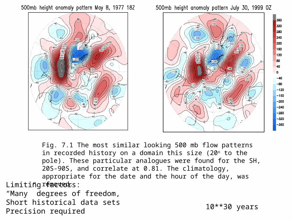
Fig. 7.1 The most similar looking 500 mb flow patterns in recorded history on a domain this size (20o to the pole). These particular analogues were found for the SH, 20S-90S, and correlate at 0.81. The climatology, appropriate for the date and the hour of the day, was removed.
10**30 years
Limiting factors:“Many” degrees of freedom,Short historical data setsPrecision required
Analogue #1 (t=0) ----’Nature’---- Analogue #1 (t)--------
Base(t=0) ---’Nature’-------------- Base(t)--------------
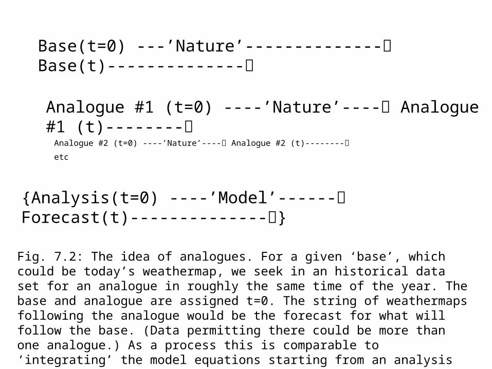
Fig. 7.2: The idea of analogues. For a given ‘base’, which could be today’s weathermap, we seek in an historical data set for an analogue in roughly the same time of the year. The base and analogue are assigned t=0. The string of weathermaps following the analogue would be the forecast for what will follow the base. (Data permitting there could be more than one analogue.) As a process this is comparable to ‘integrating’ the model equations starting from an analysis at t=0, an analysis which is as close as possible to the true base. ‘Nature’ stands for a perfect model.
{Analysis(t=0) ----’Model’------ Forecast(t)--------------}
Analogue #2 (t=0) ----’Nature’---- Analogue #2 (t)--------
etc
6. Degrees of Freedom How many degrees of freedom are evident in a physical process represented by f(s,t)?
One might think that the total number of orthogonal directions required to reproduce a data set is the dof. However, this is impractical as the dimension would increase (to infinity) with ever denser and slightly imperfect observations. Rather we need a measure that takes into account the amount of variance represented by each orthogonal direction, because some directions are more important than others. This allows truncation in EOF space without lowering the ‘effective’ dof very much.
We here think schematically of the total atmospheric or oceanic variance about the mean state as being made up by N equal additive variance processes. N can be thought of as the dimension of a phase space in which the atmospheric state at one moment in time is a point.
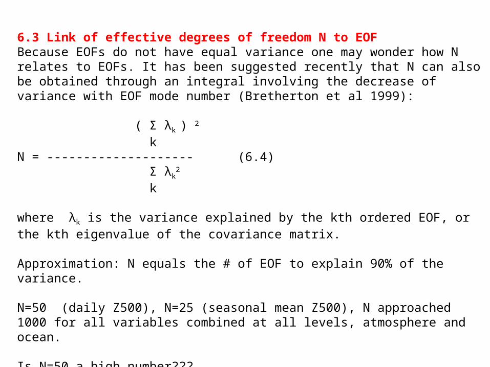
6.3 Link of effective degrees of freedom N to EOFBecause EOFs do not have equal variance one may wonder how N relates to EOFs. It has been suggested recently that N can also be obtained through an integral involving the decrease of variance with EOF mode number (Bretherton et al 1999):
( Σ λk ) 2
kN = -------------------- (6.4) Σ λk
2
k
where λk is the variance explained by the kth ordered EOF, or the kth eigenvalue of the covariance matrix.
Approximation: N equals the # of EOF to explain 90% of the variance.
N=50 (daily Z500), N=25 (seasonal mean Z500), N approached 1000 for all variables combined at all levels, atmosphere and ocean.
Is N=50 a high number???
0
5
10
15
20
25
EV
0
20
40
60
80
100
EV
-cu
mu
lative
1 2 3 4 5 6 7 8 910111213141516171819202122232425
mode number
eof
eot
eot-a
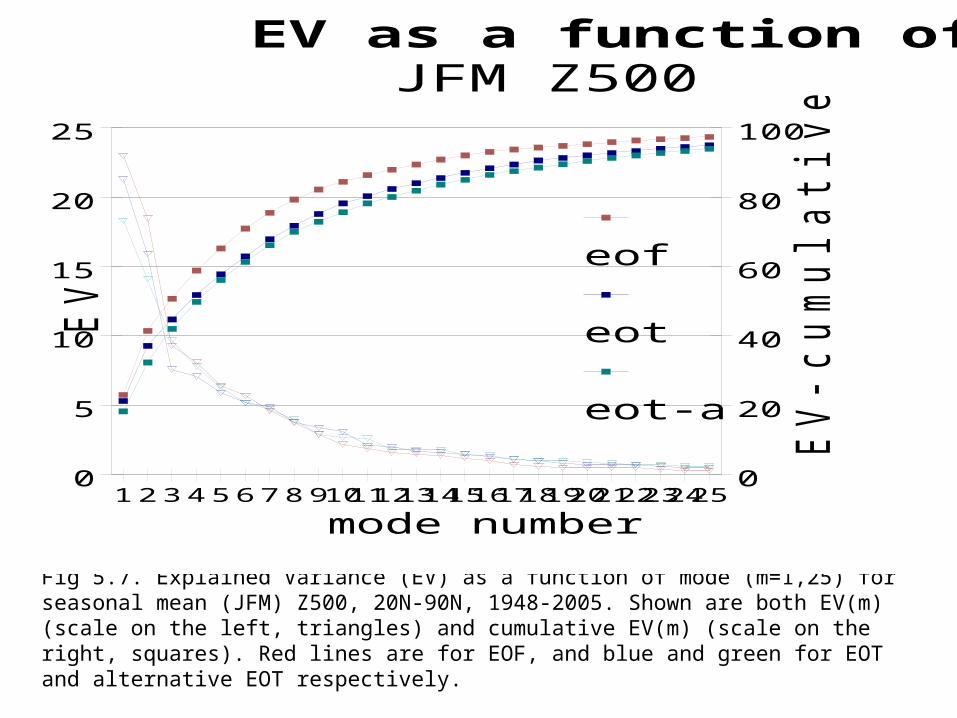
EV as a function of modeJFM Z500
Fig 5.7. Explained Variance (EV) as a function of mode (m=1,25) for seasonal mean (JFM) Z500, 20N-90N, 1948-2005. Shown are both EV(m) (scale on the left, triangles) and cumulative EV(m) (scale on the right, squares). Red lines are for EOF, and blue and green for EOT and alternative EOT respectively.

7.2 Constructed Analogues 7.2.1 The idea. Because natural analogues are highly unlikely to occur in high degree-of-freedom processes, we may benefit from constructing an analogue having greater similarity than the best natural analogue. As described in Van den Dool (1994), the construction is a linear combination of past observed anomaly patterns such that the combination is as close as desired to the initial state (or ‘base’). We then carry forward in time persisting the weights assigned to each historical case. All one needs is a data set of modest affordable length.
We do not rule out that non-linear combinations are possible, but here we report only on linear combinations.
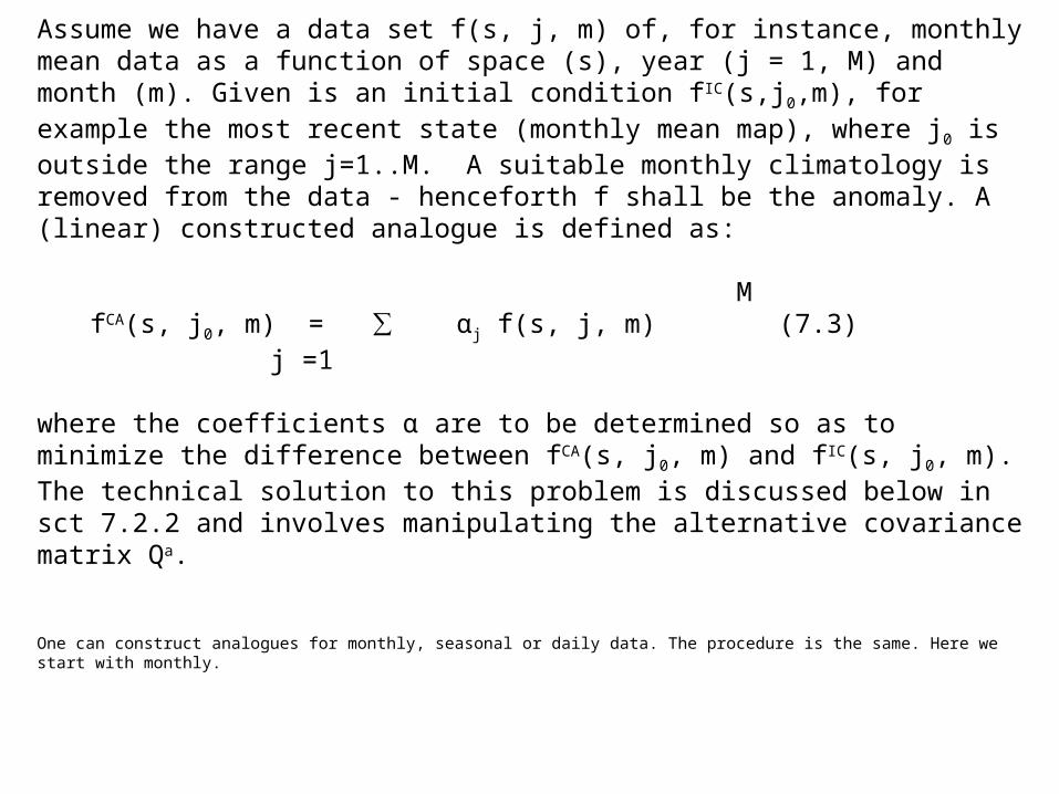
Assume we have a data set f(s, j, m) of, for instance, monthly mean data as a function of space (s), year (j = 1, M) and month (m). Given is an initial condition fIC(s,j0,m), for example the most recent state (monthly mean map), where j0 is outside the range j=1..M. A suitable monthly climatology is removed from the data - henceforth f shall be the anomaly. A (linear) constructed analogue is defined as: M
fCA(s, j0, m) = ∑ αj f(s, j, m) (7.3) j =1
where the coefficients α are to be determined so as to minimize the difference between fCA(s, j0, m) and fIC(s, j0, m). The technical solution to this problem is discussed below in sct 7.2.2 and involves manipulating the alternative covariance matrix Qa.
One can construct analogues for monthly, seasonal or daily data. The procedure is the same. Here we start with monthly.
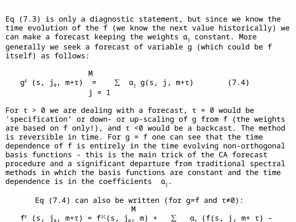
Eq (7.3) is only a diagnostic statement, but since we know the time evolution of the f (we know the next value historically) we can make a forecast keeping the weights αj constant. More generally we seek a forecast of variable g (which could be f itself) as follows:
MgF (s, j0, m+τ) = ∑ αj g(s, j, m+τ) (7.4)
j = 1
For τ > 0 we are dealing with a forecast, τ = 0 would be ‘specification’ or down- or up-scaling of g from f (the weights are based on f only!), and τ <0 would be a backcast. The method is reversible in time. For g = f one can see that the time dependence of f is entirely in the time evolving non-orthogonal basis functions - this is the main trick of the CA forecast procedure and a significant departure from traditional spectral methods in which the basis functions are constant and the time dependence is in the coefficients αj.
Eq (7.4) can also be written (for g=f and τ≠0):� M
fF (s, j0, m+τ) = fIC(s, j0, m) + ∑ αj (f(s, j, m+ τ) - f(s, j, m)) (7.4') j = 1
In this form the equation looks like a forward time stepping procedure or the discretized version of the basic equation ∂f/∂t = linear and non-linear rhs terms. Note that on the rhs of (7.4') we make linear combinations of historically observed time tendencies.
Why should Eq (7.4) yield any forecast skill? The only circumstance where one can verify the concept is to imagine we have a natural analogue. That means αj should be 1 for the natural analogue year and zero for all other years, and (7.4) simply states what we phrased already in section 7.1 and depicted in Fig 7.2, namely that two states that are close enough to be called each other’s analogue will track each other for some time and are each other’s forecast.
Obviously, no construction is required if there was a natural analogue. But, as argued in the Appendix, in the absence of natural analogues a linear combination of observed states gives an exact solution for the time tendencies associated with linear processes. There is, however, an error introduced into the CA forecast by a linear combination of tendencies associated with purely non-linear components, and so a verification of CA is a statement as to how linear the problem is. Large scale wave propagation is linear, and once one linearizes wrt some climatological mean flow the linear part of the advection terms may be larger than the non-linear terms. This is different for each physical problem.
Is a constructed analogue linear? The definition in (7.4) is a linear combination of non-linearly evolving states observed in the past. So even in (7.4) itself there is empirical non-linearity. Moreover, in section 7.6, we will change the weights during the integration expressed in (7.4') - this will add more to non-linearity. (We are not reporting on any attempts to add quadratic terms in (7.4) - that would allow for more substantial non-linearity, but the procedure to follow is unclear).
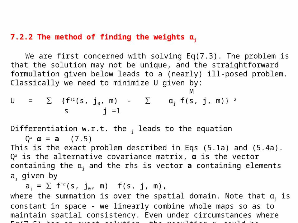
7.2.2 The method of finding the weights αj
We are first concerned with solving Eq(7.3). The problem is that the solution may not be unique, and the straightforward formulation given below leads to a (nearly) ill-posed problem. Classically we need to minimize U given by: MU = ∑ {fIC(s, j0, m) - ∑ αj f(s, j, m)} 2 s j =1 Differentiation w.r.t. the j leads to the equation
Qa α = a (7.5)This is the exact problem described in Eqs (5.1a) and (5.4a). Qa is the alternative covariance matrix, α is the vector containing the αj and the rhs is vector a containing elements aj given by
aj = ∑ fIC(s, j0, m) f(s, j, m), where the summation is over the spatial domain. Note that αj is constant in space - we linearly combine whole maps so as to maintain spatial consistency. Even under circumstances where Eq(7.5) has an exact solution, the resulting αj could be meaningless for further application, when the weights are too large, and ultra-sensitive to a slight change in formulating the problem.
A solution to this sensitivity, suggested by experience, consists of two steps:1) truncate fIC(s, j0, m) and all f(s, j, m) to about M/2 EOFs. Calculate Qa and rhs vector a from the truncated data. This reduces considerably the number of orthogonal directions without lowering the EV (or effective degrees of freedom N) very much.2) enhance the diagonal elements of Qa by a small positive amount (like 5% of the mean diagional elements), while leaving the off-diagonal elements unchanged. This procedure might be described as the controlled use of the noise that was truncated in step 1.
Increasing the diagonal elements of Qa is a process called ridging. The purpose of ridge regression is to find a reasonable solution for an underdetermined system (Tikhonov 1977; Draper and Smith 1981). In the version of ridge regression used here the residual U is minimized but subject to minimizing ∑αj
2 as well. The latter constraint takes care of unreasonably large and unstable weights. One needs to keep the amount of ridging small. For the examples discussed below the amounts added to the diagonal elements of Qa is continued until ∑α j
2 <0.5.
One can raise the question about which years to pick, thus facing a near infinity of possibilities to chose from. Here we will use all years. No perfect approach can be claimed here, and the interested reader may invent something better. A large variety of details about ridging is being developed in various fields (Green and Silberman 1994; Chandrasekaran and Schubert 2005), see also appendix of chapter 8.
Note that the calculation of α(t) has nothing to do with Δt or future states of f or g, so the forecast method is intuitive, and not based on minimizing some rms error for lead Δt forecasts. There could not possibly be an overfit on the predictand. Or could there?
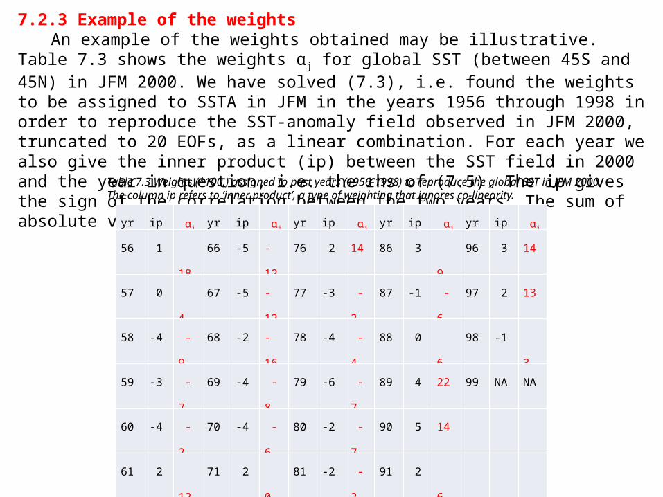
7.2.3 Example of the weightsAn example of the weights obtained may be illustrative. Table 7.3 shows the weights
αj for global SST (between 45S and 45N) in JFM 2000. We have solved (7.3), i.e. found the weights to be assigned to SSTA in JFM in the years 1956 through 1998 in order to reproduce the SST-anomaly field observed in JFM 2000, truncated to 20 EOFs, as a linear combination. For each year we also give the inner product (ip) between the SST field in 2000 and the year in question, i.e. the rhs of (7.5). The ip gives the sign of the correlation between the two years. The sum of absolute values of ip is set to 1.
yr ip αj yr ip αj yr ip αj yr ip αj yr ip αj
56 1 18 66 -5 -12 76 2 14 86 3 9 96 3 14
57 0 4 67 -5 -12 77 -3 -2 87 -1 -6 97 2 13
58 -4 -9 68 -2 -16 78 -4 -4 88 0 6 98 -1 3
59 -3 -7 69 -4 -8 79 -6 -7 89 4 22 99 NA NA
60 -4 -2 70 -4 -6 80 -2 -7 90 5 14
61 2 12 71 2 0 81 -2 -2 91 2 6
62 -1 -1 72 1 -2 82 1 -3 92 0 18
63 -1 2 73 -2 3 83 -1 -5 93 -1 -17
64 -4 0 74 3 8 84 1 15 94 0 -6
65 -1 -19 75 1 0 85 5 6 95 0 1
Table 7.3 Weights (*100.) assigned to past years (1956-1998) to reproduce the global SST in JFM 2000. The column ip refers to ‘inner product’, a type of weighting that ignores co-linearity.
Below we will discuss applications to demonstrate how well constructed analogues (CA) work.
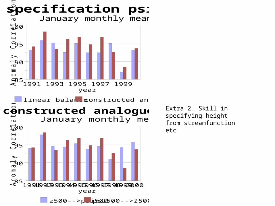
The first example is specification of monthly mean surface weather from 500mb streamfunction.
In section 7.4 we describe global SST forecasts - this has been the main application of CA so far.
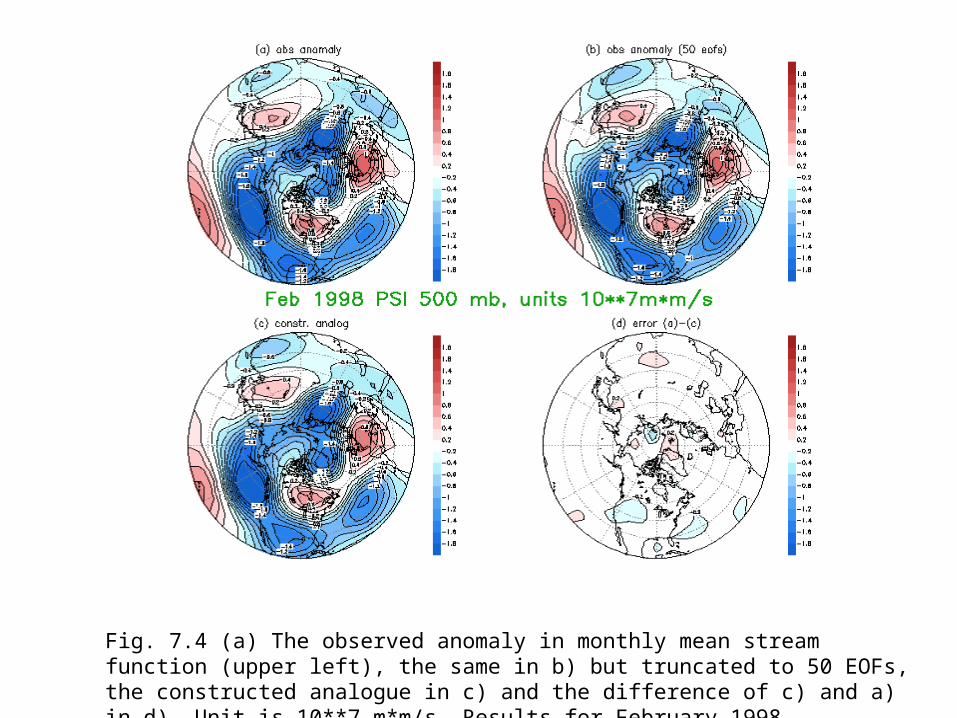
Fig. 7.4 (a) The observed anomaly in monthly mean stream function (upper left), the same in b) but truncated to 50 EOFs, the constructed analogue in c) and the difference of c) and a) in d). Unit is 10**7 m*m/s. Results for February 1998.
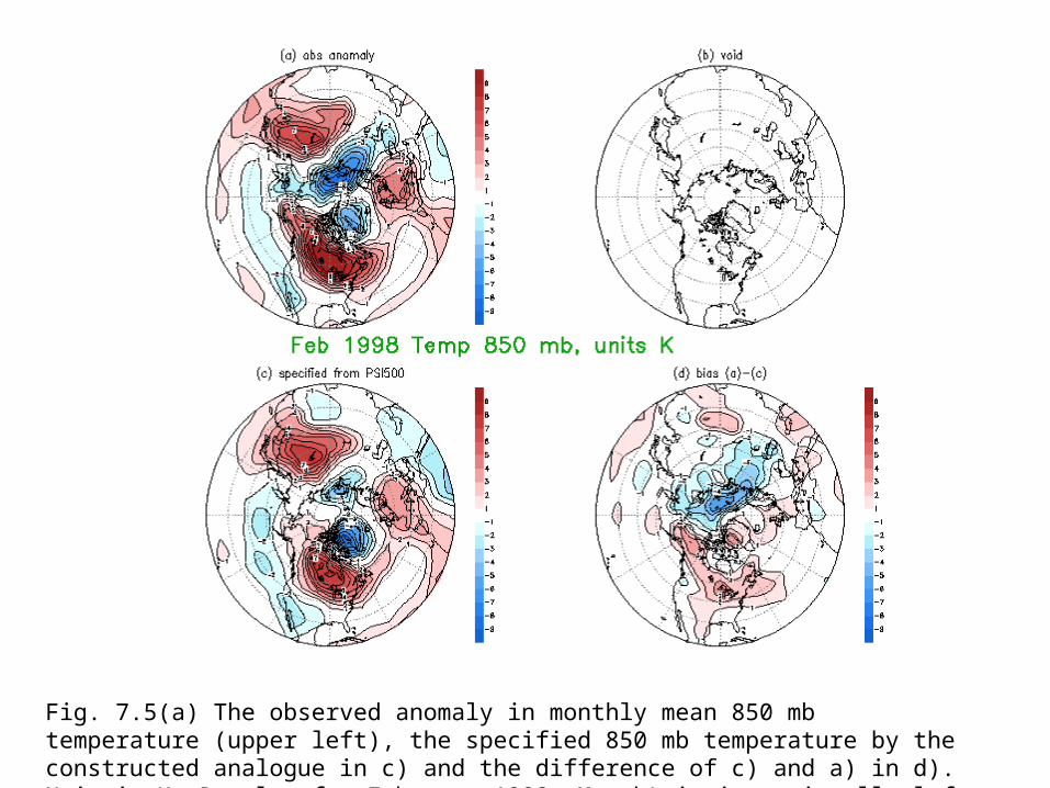
Fig. 7.5(a) The observed anomaly in monthly mean 850 mb temperature (upper left), the specified 850 mb temperature by the constructed analogue in c) and the difference of c) and a) in d). Unit is K. Results for February 1998. Map b) is intentionally left void.
85
90
95
100
Anom
aly
Corr
ela
tion (
X 1
00)
1991 1993 1995 1997 1999year
linear balance constructed analogue
specification psi500-->Z500January monthly mean
85
90
95
100
Anom
aly
Corr
ela
tion (
X 1
00)
1991199219931994199519961997199819992000year
z500-->psi500psi500-->Z500
constructed analogue specificationJanuary monthly mean
Extra 2. Skill in specifying height from streamfunction etc
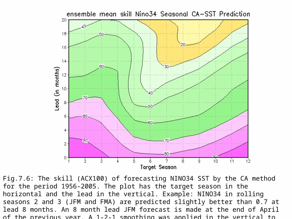
Fig.7.6: The skill (ACX100) of forecasting NINO34 SST by the CA method for the period 1956-2005. The plot has the target season in the horizontal and the lead in the vertical. Example: NINO34 in rolling seasons 2 and 3 (JFM and FMA) are predicted slightly better than 0.7 at lead 8 months. An 8 month lead JFM forecast is made at the end of April of the previous year. A 1-2-1 smoothing was applied in the vertical to reduce noise.
-1.5
-1
-0.5
0
0.5
1
1.5
SS
T-a
no
ma
ly in
de
gre
e C
djf mam05 jja son05 djf mam06 jja06 son06 djfseason
ca12_16_e
OBS
ca12_16_l
ca12_21_e
ca12_21_l
ca1_21_e
ca1_21_l
ca1_16_e
ca1_16_l
ca1_26_e
ca1_26_l
ca12_26_e
ca12_26_l
ens_ave
12 MmbrEnsemble CA Forecast Nino3.4data thru Jun 2005
Fig. 7.7 An ensemble of 12 forecasts for Nino34. The release time is July 2005, data through the end of June were used. Observations (3 mo means) for the most recent 6 overlapping seasons are shown also. The ensemble mean is the black line with closed circles. The CA ensemble members were created by different EOF truncation etc (see text).
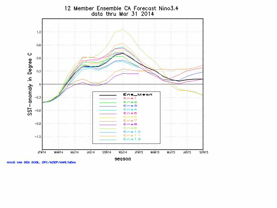
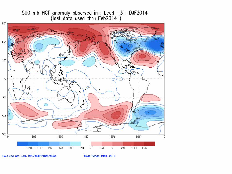
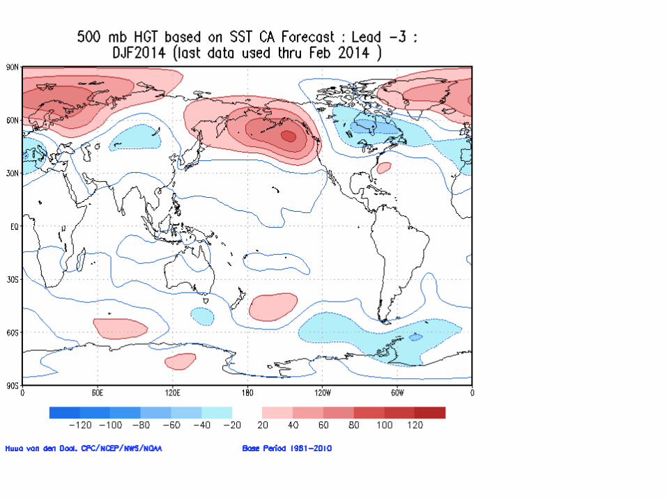
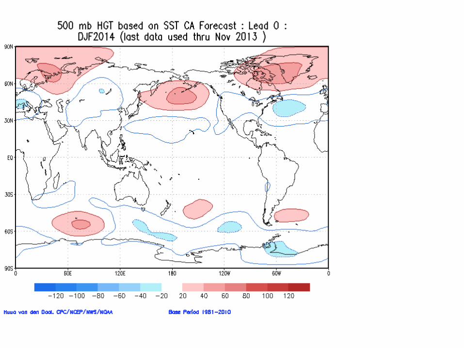
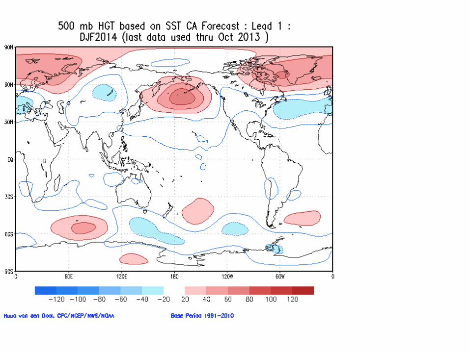
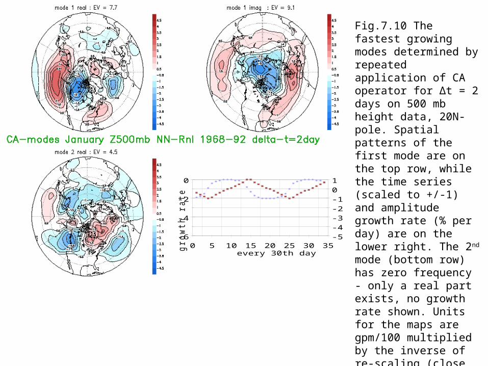
Fig.7.10 The fastest growing modes determined by repeated application of CA operator for Δt = 2 days on 500 mb height data, 20N-pole. Spatial patterns of the first mode are on the top row, while the time series (scaled to +/-1) and amplitude growth rate (% per day) are on the lower right. The 2nd mode (bottom row) has zero frequency - only a real part exists, no growth rate shown. Units for the maps are gpm/100 multiplied by the inverse of re-scaling (close to unity usually) applied to the time series. .
-6
-4
-2
0g
row
th r
ate
-5
-4
-3
-2
-1
0
1
a
mp
litu
de
0 5 10 15 20 25 30 35every 30th day
real part imaginary partgrowth rate
time series and growth ratemode#1 in daily 0Z Z500 - deltat=2 day


![A Dimensions: [mm] B Recommended land pattern: [mm] D ... · 2013-03-12 2013-01-13 2012-12-10 2012-10-29 2012-08-27 2006-05-05 DATE SSt SSt SSt SSt SSt SSt SSt BY SSt COt COt SSt](https://img.pdfslide.us/doc/110x75/604b228bc93c005c75431c51/a-dimensions-mm-b-recommended-land-pattern-mm-d-2013-03-12-2013-01-13.jpg)


![A Dimensions: [mm] B Recommended land pattern: [mm] D ... · 2005-12-16 DATE SSt SSt SSt SSt SSt SSt SSt BY SSt SSt SMu SMu SSt ... RDC Value 600 800 1000 0.20 High Cur rent ... 350](https://img.pdfslide.us/doc/110x75/5c61318009d3f21c6d8cb002/a-dimensions-mm-b-recommended-land-pattern-mm-d-2005-12-16-date-sst.jpg)


![A Dimensions: [mm] B Recommended land pattern: [mm] · 2020. 8. 11. · 2014-03-11 2013-12-19 2013-12-04 2013-04-10 2013-03-06 2013-02-14 2012-12-10 DATE SSt SSt SSt SSt SSt SSt SSt](https://img.pdfslide.us/doc/110x75/6145e75a8f9ff812541fec6f/a-dimensions-mm-b-recommended-land-pattern-mm-2020-8-11-2014-03-11-2013-12-19.jpg)