2008 International ANSYS Conference · PDF file1 E-Z-GO Proprietary 2008 International ANSYS Conference Optimization Design for Multiple Loads with ANSYS Jing Heng Wen Senior Project

1 E-Z-GO Proprietary

2008 International ANSYS Conference

Optimization Design for Multiple Loads with ANSYS

Jing Heng WenSenior Project EngineerE-Z-GO, A Textron Company


+

Cost/Weight Reduction

Optimization Process Introduction


Input Variable

Geo

met

ry D

imen

sion High Quality

CAD Import

Other Format Import

Bring in Dim. Parameters

W/o Dim. Parameter

DOE

Optimization

Topological

Create Dim. Parameters in FEA

Other Factor

Force Torque Temperature in FEA

Failure Root Cause Correlate with test Max. allowed load

FEM

Geometric Parameterization

• Importing geometry with useful dimension parameters is very helpful for FEA Optimization, but is not restricted


Optimization Analysis with ANSYS Build-in Tools

• Single Objective Optimization Analysis – Correlating simplifying FEA model with test data for model accuracy– Test data processing with 3rd software to determine multiple load

cases– Simplify complex assembly with some simple FEM elements– Set various assumptions for easy modeling & fast solution

• Topological Analysis – Shape Determination– Completing with multiple loading cases with different analyzing

weighting in one solution– Determining shape with defined percentage of volume reduction– No geometry dimension parameters required

• DOE, Goal Driven – Numerical Determination– Determine best input variables combination numerically for output

goals– Trade-off tool is used to determine design variable under multiple

loadings for finalizing


Optimization Design for Multiple Loads with ANSYS

• Correlating Simplifying FEA Model with Test Data– Three Major Challenges to FEA

• Accuracy: Better Modeling, quality meshing and proper loadings/boundary Conditions

• Timing: Short modeling period and fast/reliable solution • Cost: Labor cost and computer resource cost

– To Meet Accuracy Challenges:• Correlate model with test data, Modeling V&V (Objective)• Optimize analysis for model V&V to meet both accuracy and

timing challenges• Others, such as element quality

– To Meet Timing and Cost Challenges, We often• Simplify complex assembly with some simple FEM elements

sometimes, even drop some components based on the judgments• Set various assumptions for easy modeling & fast solution


1-1. Processing Test Data to Determine Multiple Loads vs. Strain

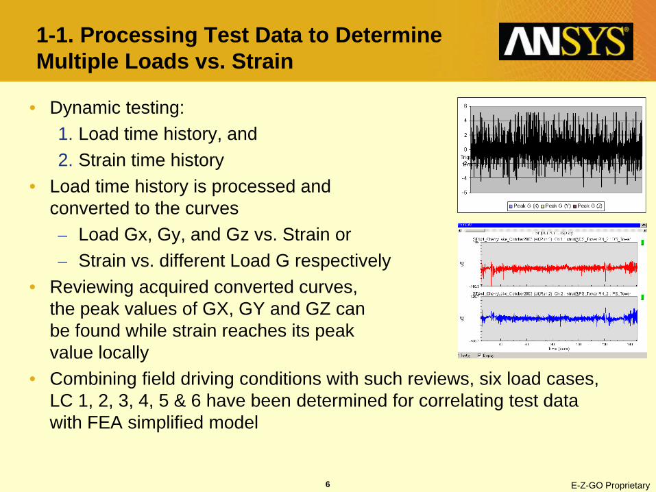
• Dynamic testing: 1. Load time history, and 2. Strain time history

• Load time history is processed and converted to the curves– Load Gx, Gy, and Gz vs. Strain or – Strain vs. different Load G respectively

• Reviewing acquired converted curves, the peak values of GX, GY and GZ can be found while strain reaches its peak value locally

• Combining field driving conditions with such reviews, six load cases, LC 1, 2, 3, 4, 5 & 6 have been determined for correlating test data with FEA simplified model


1-2. Simplifying FEA Model with Correlated Multiple Boundary Condition

• Simplifying RXV frame sub-assembly – Its components are built by shell or solid elements– Revolute, slide and universal joints used for front and rear

suspension are made by constraint elements– Spring damp elements and beam elements are added where are

required• Ground loads transfer to components are often different than theoretical

prediction plus our FEA model is also simplified– So the major issue becomes how to correlate FEA model with field

test data– Optimization analysis will help us to correlate

• The model is used for correlating test data, so meshing in those areas is observed closely


1-3. Optimize - Approximation Method and its Settings

• Sub-Problem Approximation:– Zero-order method solving most engineering problem with single

minimized Objective (OBJ)– Other measures: State Variable (SV), Design Variable (DV)

• DV: Input factors are what DOE looks for, DOE result for DV is a group of best inputs to reach the goals. Simultaneous Smax1, Smax2, Smax3 are defined as DV

• SV and OBJ: Both are Measures– OBJ: The single goal of DOE at each loop, is always minimized

• Such as reciprocal of Smax1 (w/ peak value), is set OBJ– SV: Constrain solution

• All measures which can not be set as a OBJ. (Smax2, Smax3); – The measure, which is used for OBJ, is also set as SV with two

equalities (max./min.) to restrict its value for accessible result


1-4. Input and Output Variables Determinations• DV Setting

– Six unknown input loads FX1, FY1, FZ1, FX2, FY2 & FZ2 on the end of front axle/rear axle

– DV range: positive, based on judgment/test data

• SV Setting– Simultaneous 3 – 6 stress targets at key locations are required– The smaller the SV variation is, the better correlation will be

• Such as for LC 1, Smax2 is targeted at 13.2 +/-3%, Smax3 is 11.3 +/-3%

• SV number and Range set depends on feasible sets – Treat one key target test data, Smax1, equally with two SVs

• OBJ (Objective function) Setting – Obj-Smax1, a reciprocal of Smax1, is set and let Optimize to

minimize


Smax1: 45 Smax2: 13.2 Smax3: 11.3

FX1FY2

FZ1FX2

FY1FZ2

1-5. Results of Correlating FEA Model with Field Test Data

• The load is used for sub-assembly, front suspension analysis with A-Arm, because same methodology is used for its FEA simplifying and assumption

• Optimized / Correlated loads are recorded as standard BC for future design


Che

ck 2

ndA

rea

Stre

ss

Summary: Correlating FEA Model w/Test Data (Multiple Peak)

1. Defining six peak load casesdetermined by driving condition & converted curve - load vs. strain with processing load-time and strain-time; (manipulating static rolling, braking over bumper, wheeling in pothole, cornering)

2. Run optimization analysis with Sub-problem to acquire OPT load (F and MG) for each LC;

3. Run six different load cases 4. Check the strain/stress at 2nd

area to adjust SV range for higher confidence level of OPT loads;


2. Optimization Analysis for A-Arm with Multiple Loads

• Objective: Weight/Cost Reduction• Component: A-Arm (Front Suspension)

– Objective: 1. Volume reducing 30%, 2. Stress reducing 15% under LC 1 – Bumper Dyno;

Similar stress under other loading cases3. Sub-assembly tolerance control (from weldment to casting)

A. Topological: • Shape Determining with multiple loads• Multiple loads with different counting weighing for certain

percentage volume reductionB. DOE:

• Numerical Determination • CCD, Goal Driven Optimization for multiple objectives under

selected two key load cases


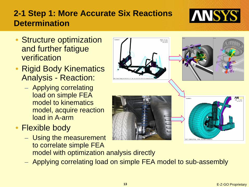
2-1 Step 1: More Accurate Six Reactions Determination

• Structure optimization and further fatigue verification

• Rigid Body Kinematics Analysis - Reaction: – Applying correlating

load on simple FEA model to kinematics model, acquire reaction load in A-arm

• Flexible body– Using the measurement

to correlate simple FEA model with optimization analysis directly

– Applying correlating load on simple FEA model to sub-assembly


2-2. Step 2 – Topological, Shape

• Multiple loads in one solution:– Dyno:Crash:Torsion:Twist

= 40:20:20:20 (%)• Volume Reduction: 30%

– Blue, Green and yellow colors represent the area that could be cut and built into different shapes

• It is very helpful: – Determine % volume reduction, in

order to support MOO, in which the numerical amount of volume cannot be set as a target directly in most cases with GDO when conflicting stress is targeted numerically

– Multiple load cases with different fatigue life requirement


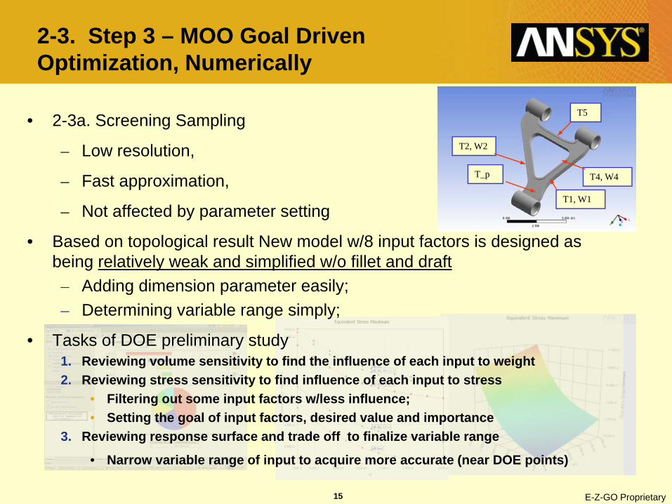
2-3. Step 3 – MOO Goal Driven Optimization, Numerically

• 2-3a. Screening Sampling

– Low resolution,

– Fast approximation,

– Not affected by parameter setting

• Based on topological result New model w/8 input factors is designed as being relatively weak and simplified w/o fillet and draft– Adding dimension parameter easily;– Determining variable range simply;

• Tasks of DOE preliminary study1. Reviewing volume sensitivity to find the influence of each input to weight2. Reviewing stress sensitivity to find influence of each input to stress

• Filtering out some input factors w/less influence;• Setting the goal of input factors, desired value and importance

3. Reviewing response surface and trade off to finalize variable range

• Narrow variable range of input to acquire more accurate (near DOE points)

T2, W2

T5

T_p

T1, W1

T4, W4


Input Variable and Objective (Measure) Determination (1)

OBJ DV Sensit ivity DV/OBJ Value

V Stress Range Sett ing

LC 4 LC 7 Low Up Init .

T1 1(0.5) 3(5) 1

W1 1 4 2

T2 1(0.5) 3(5) 1

W2 1 4 2

T3 0.5 2(3) 1

W3 1 4 2

T4 0.5 5 1

T_P 0 1 0

V (DOE) Smallest

σ (DOE) LC1/L 2: <310 / <375

V (Original) 30% Cut 1.47 2.10

σ (Original) LC2: 340 LC1 15% Cut, 285 Dyno: 331 / Crash: 345

DV Setting (Relative weak model) OBJ Setting (Current : New)

Stress - 331 : 285 (LC 1, Life up 20%)345 : 340 (LC 2, no change)

Due to FEA DOE model w/o fillet/shaft, Stress up ~10%: 285/340 to 310/375

Initial to higher, Same for 2 loads Volume - 2.10 : 1.47 (30% Cut)This numerical target is difficult to get feasible result when it is set in GDO MOO. Because no single point that could be set as the best value for two or more mutually conflicting objective. If it happens, set volume goal “as smaller at possible” at first, using trade off technique to get numerical target next.

2-3a. Screening Sampling (Continue)


OBJ DV Sensit ivity DV/OBJ Value DOE Value

V Stress Range Sett ing Value Bound/

LC 4 LC 7 Low Up Init . Importance LC 2 LC 1

T1 0.38 -0.32 -0.81 1(0.5) 3(5) 1

W1 0.31 -0.42 -0.15 1 4 2

T2 0.47 -0.75 -0.29 1(0.5) 3(5) 1

W2 0.25 -0.09 -0.44 1 4 2

T3 0.26 -0.04 -0.07 0.5 2(3) 1

W3 0.18 0.00 0.00

T4 0.11 -0.01 -0.02

T_P 0.61 -0.25 -0.12 0 1 0

V (DOE) Smallest

σ (DOE) LC1/L 2: <310 / <375


σ (Original) LC2 same LC1 15% Cut, 285 Dyno: 331 / Crash: 345

Upper/High

NoPref/Def.

Upper/High

NoPref/Def.

NoPref/Low

en

en

Lower/High

Filter out in screen


Reviewing sensitivity

• Filter out unimportant input: W3, T4

Viewing response surface & trade-off

• Narrow variable range when measure can be restricted at certain range

• Define input goals: Desired value (lower/Upper/Mid / No Preference) & Importance (Higher/Lower/Default)

Goal Settings (Detail see next)

2-3b. Advanced Sampling

• More refined approximation, Max. allowable Pareto % : 65-70, affected by parameter settings


Rerun DOE w/Advanced Sampling

Goal Settings for Feasible Set (cont.)

(1) Higher sensitive to stress: “Near upper Bound”, “Higher” Importance; (2) Lower sensitive to stress/volume: “Near lower bound”, “Lower” importance. (3) Higher sensitive to volume; “Near lower bound”, “Higher” importance; (4) Mixture sensitive to volume and stress: “No preference”(“Mid point”) , “Default” importance; (5) Same DV setting for two loads; (6) Limited number set at “Higher” Importance;

2. DV Goal Setting:

1. OBJ Goal Setting (Conflict):(1) Stress: Numerical target – “less than” target and “higher” importance. (Reliability) (2) Volume: “Minimum possible”, “Default” importance. ( Topological, Trade-off)

3. Adjust goals, if no feasible set is acquired or too many feasible sets are acquired

OBJ DV Sensit ivity DV/OBJ Value DOE Value

V Stress Range Sett ing Value Bound/

LC 4 LC 7 Low Up Init . Importance LC 2 LC 1

T1 0.38 -0.32 -0.81 1(0.5) 3(5) 1

W1 0.31 -0.42 -0.15 1 4 2

T2 0.47 -0.75 -0.29 1(0.5) 3(5) 1

W2 0.25 -0.09 -0.44 1 4 2

T3 0.26 -0.04 -0.07 0.5 2(3) 1

W3 0.18 0.00 0.00

T4 0.11 -0.01 -0.02

T_P 0.61 -0.25 -0.12 0 1 0

V (DOE) Smallest

σ (DOE) LC1/L 2: <310 / <375



Upper/High

NoPref/Def.

Upper/High

NoPref/Def.

Lower/Low

en

en

Lower/High



1.94 2.92

2.84 2.64

1.98 0.51

2.63 2.59

1.58 1.72

N/A N/A

N/A N/A

0.03 0.02

1.47 1.15

375 307

2-3b. Advanced Sampling (Continue)


Trade-off is very useful for:

• Multi load cases (solutions)

• Multi objective in one solution. Because setting numerical target for mutually conflicting objectives brings infeasible set (result)

Picking one point, which is close to defined volume setting with corresponding stress as low as possible, a group input variables is shown in left column.

V

S

Typing the best input values (acquired from LC 1) into left column of trade off picture (acquired from LC 2), a responding point will show in right picture. Adjust several times (2-3 times), the best point can be found to satisfy both loads.

Value of Input factor

( Note: This trade off is acquired by screening sampling method)

2-3c. Trade-off Tech. w/DOE Response Surface, Regression Fitting


Based on acquired two DOE results from LC1 and LC 2, volume and stress are traded off and the values of input factors are defined.

OBJ DV Sensit ivity DV/OBJ Value DOE Value DOE

V Stress Range Sett ing Value Bound/ Validat ion

LC 4 LC 7 Low Up Init . Importance LC 2 LC 1 (Final)

T1 0.38 -0.32 -0.81 1(0.5) 3(5) 1

W1 0.31 -0.42 -0.15 1 4 2

T2 0.47 -0.75 -0.29 1(0.5) 3(5) 1

W2 0.25 -0.09 -0.44 1 4 2

T3 0.26 -0.04 -0.07 0.5 2(3) 1

W3 0.18 0.00 0.00 Filter out in screen

T4 0.11 -0.01 -0.02 Filter out in screen

T_P 0.61 -0.25 -0.12 0 1 0

V (DOE) Smallest

σ (DOE) LC1/L 2: <310 / <375



Upper/High

NoPref/Def.

Upper/High

NoPref/Def.

NoPref /Low

en

en

Lower/High

1.94 2.92

2.84 2.64

1.98 0.51

2.63 2.59

1.58 1.72

N/A N/A

N/A N/A

0.03 0.02

1.47 1.15

375 307

3 .0 0

2 .75

2 .0 0

2 .75

1.75

2 .0 0

1.0 0

0 .0 0

1.49

285/375

These values are rounded to meet manufacturing needs.DOE Model Validation: GDO algorithm works off of its DOE response surface, so the final input combination should be validated in DOE last process. The validation process is submitting the input combination as hard design points and running the solution.DOE Model Validation Results

The validating results are: V=1.485 for both load cases ( Target is V=1.47)LC 1 σ=285 (target σ =310); LC 2 σ =375 (Target σ =375)

2-4. Step 4. Validate DOE Model with Input Value Defined by 2 Loads (Static structure)


OBJ DV Sensit ivity DV/OBJ Value DOE Value DOE Verif icat ion

V Stress Range Sett ing Value Bound/ Validat ion Correlat ion

LC 4 LC 7 Low Up Init . Importance LC 2 LC 1 (Final)

T1 0.38 -0.32 -0.81 1(0.5) 3(5) 1

W1 0.31 -0.42 -0.15 1 4 2

T2 0.47 -0.75 -0.29 1(0.5) 3(5) 1

W2 0.25 -0.09 -0.44 1 4 2

T3 0.26 -0.04 -0.07 0.5 2(3) 1

W3 0.18 0.00 0.00 Filter out in screen

T4 0.11 -0.01 -0.02 Filter out in screen

T_P 0.61 -0.25 -0.12 0 1 0

V (DOE) Smallest

σ (DOE) LC1/L 2: <310 / <375



Upper/High

NoPref/Def.

Upper/High

NoPref/Def.

NoPref /Low

en

en

Lower/High

1.94 2.92

2.84 2.64

1.98 0.51

2.63 2.59

1.58 1.72

N/A N/A

N/A N/A

0.03 0.02

1.47 1.15

375 307

3 .0 0

2 .75

2 .0 0

2 .75

1.75

2 .0 0

1.0 0

0 .0 0

3 .0 0

2 .75

2 .0 0

2 .75

1.75

2 .0 0

1.0 0

0 .0 0

1.49

285/375

1.48

286/337

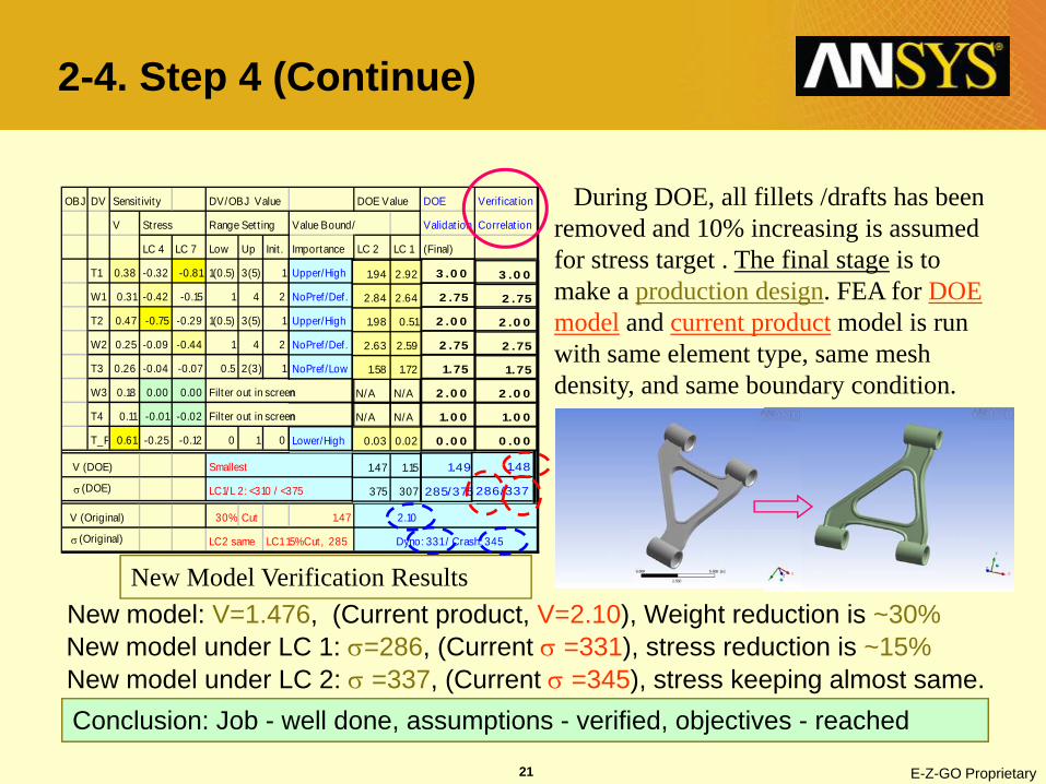
During DOE, all fillets /drafts has been removed and 10% increasing is assumed for stress target . The final stage is to make a production design. FEA for DOE model and current product model is run with same element type, same mesh density, and same boundary condition.

New Model Verification ResultsNew model: V=1.476, (Current product, V=2.10), Weight reduction is ~30%New model under LC 1: σ=286, (Current σ =331), stress reduction is ~15%New model under LC 2: σ =337, (Current σ =345), stress keeping almost same.Conclusion: Job - well done, assumptions - verified, objectives - reached

2-4. Step 4 (Continue)


3-1. Introduction of Loading Scale K:To ensure a reasonable loading environment,(1) The measured load magnitude is different from the correlated load.(2) N-S curve is not exact linearUsing original load history will overkill estimation The value of K:Initial value of K: K= (OPT Load value) / (Peak value from corresponding test data).K will be adjusted after comparing life prediction with actual test result for current frame.

3-2. The method to estimate fatigue:(1) Stress-Life approach (S-N); for high-cycle(2) Strain-Life approach (E-N). for both long life/high cycles and short life/low cycle.Considering the exist of severe loadings, E-N is chosen for the estimation.

Current A-arm Test

Current A-arm FEA Model

New A-arm FEA Model

3. Verifying New Design w/Fatigue


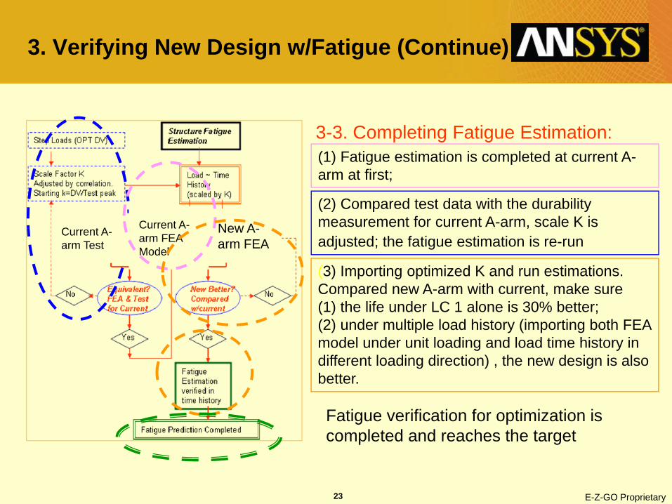
3-3. Completing Fatigue Estimation:(1) Fatigue estimation is completed at current A-arm at first;

(2) Compared test data with the durability measurement for current A-arm, scale K is adjusted; the fatigue estimation is re-run

(3) Importing optimized K and run estimations. Compared new A-arm with current, make sure (1) the life under LC 1 alone is 30% better; (2) under multiple load history (importing both FEA model under unit loading and load time history in different loading direction) , the new design is also better.

New A-arm FEA

Current A-arm FEA Model

Current A-arm Test

Fatigue verification for optimization is completed and reaches the target

3. Verifying New Design w/Fatigue (Continue)


FEA results under unit loading in 3 directions

Three loading-time histories with adjusted scale K

EN Analyzer Damage Result

Data Value

Appendix 2: Fatigue Estimation Process, DOE A-Arm Life Validation


Conclusion and Acknowledgements

• FEA with optimization process has been proven very useful in virtual vehicle manufacturing world for cost and time saving– With ANSYS built in tools, running optimization analysis for multiple

load cases is powerful and easy to handle and understanding

• The author is indebted to many colleagues in E-Z-GO Engineering Design, R&D lab and Communication Department

Documents

2008 International ANSYS Conference · PDF file1 E-Z-GO Proprietary 2008 International ANSYS Conference Optimization Design for Multiple Loads with ANSYS Jing Heng Wen Senior Project