Externalities

131 Undergraduate Public Economics

Emmanuel Saez

UC Berkeley

1

OUTLINE

Second part of course is going to cover market failures and

show how government interventions can help

1) Externalities and public goods

2) Asymmetric information (social insurance)

3) Individual failures (savings for retirement)

2

EXTERNALITIES

Market failure: A problem that violates one of the assump-tions of the 1st welfare theorem and causes the market econ-omy to deliver an outcome that does not maximize efficiency

Externality: Externalities arise whenever the actions of oneeconomic agent directly affect another economic agent out-side the market mechanism

Externality example: a steel plant that pollutes a river usedfor recreation

Not an externality example: a steel plant uses more electricityand bids up the price of electricity for other electricity cus-tomers

Externalities are one important case of market failure

3

EXTERNALITY THEORY: ECONOMICS OFNEGATIVE PRODUCTION EXTERNALITIES

Negative production externality: When a firm’s productionreduces the well-being of others who are not compensated bythe firm.

Private marginal cost (PMC): The direct cost to producersof producing an additional unit of a good

Marginal Damage (MD): Any additional costs associatedwith the production of the good that are imposed on othersbut that producers do not pay

Social marginal cost (SMC = PMC + MD): The privatemarginal cost to producers plus marginal damage

Example: steel plant pollutes a river but plant does not faceany pollution regulation (and hence ignores pollution whendeciding how much to produce)

4

Public Finance and Public Policy Jonathan Gruber Fourth Edition Copyright © 2012 Worth Publishers 10 of 35

C H A P T E R 5 ■ E X T E R N A L I T I E S : P R O B L E M S A N D S O L U T I O N S

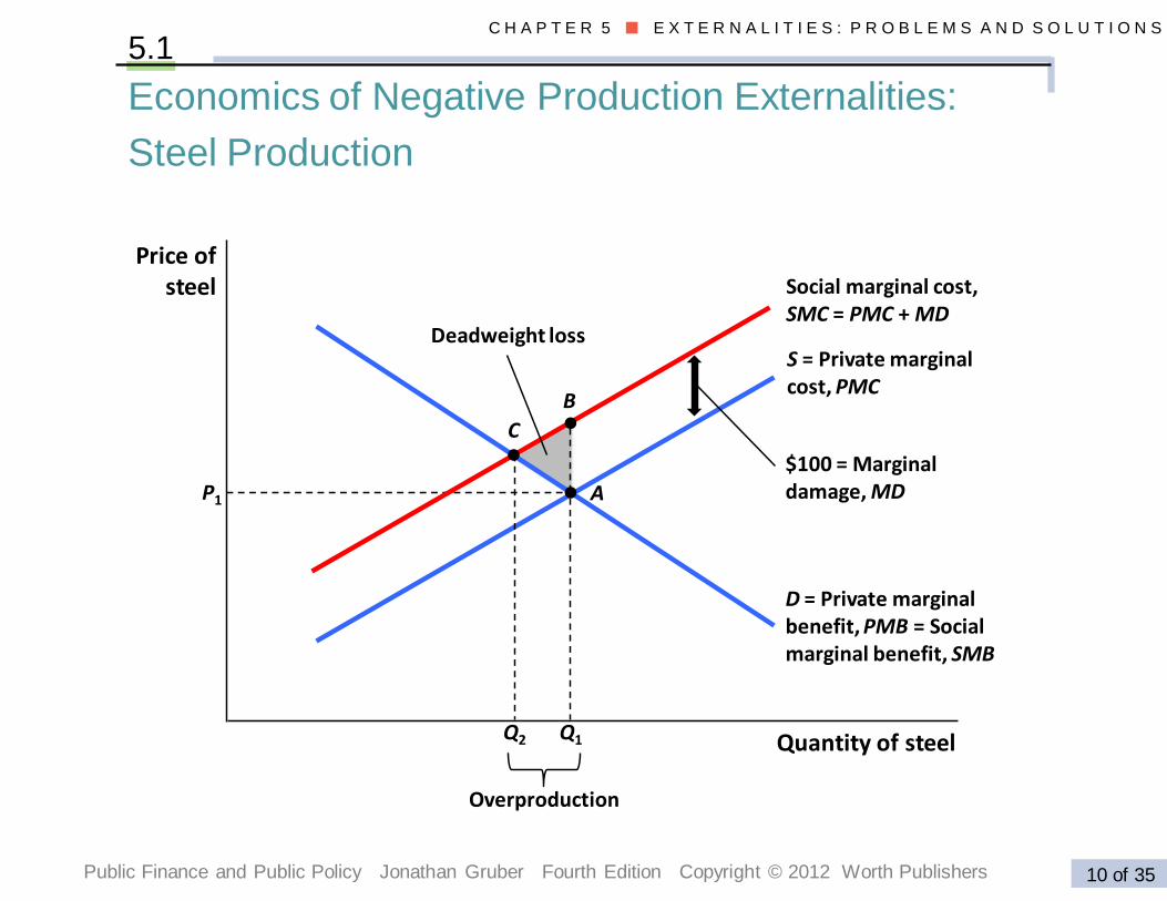
Economics of Negative Production Externalities:

Steel Production

5.1

Price ofsteel

Quantity of steel

B

C

A

Q1Q2

P1

Deadweight loss

Social marginal cost, SMC = PMC + MD

S = Private marginal cost, PMC

$100 = Marginal damage, MD

D = Private marginal benefit, PMB = Social marginal benefit, SMB

Overproduction

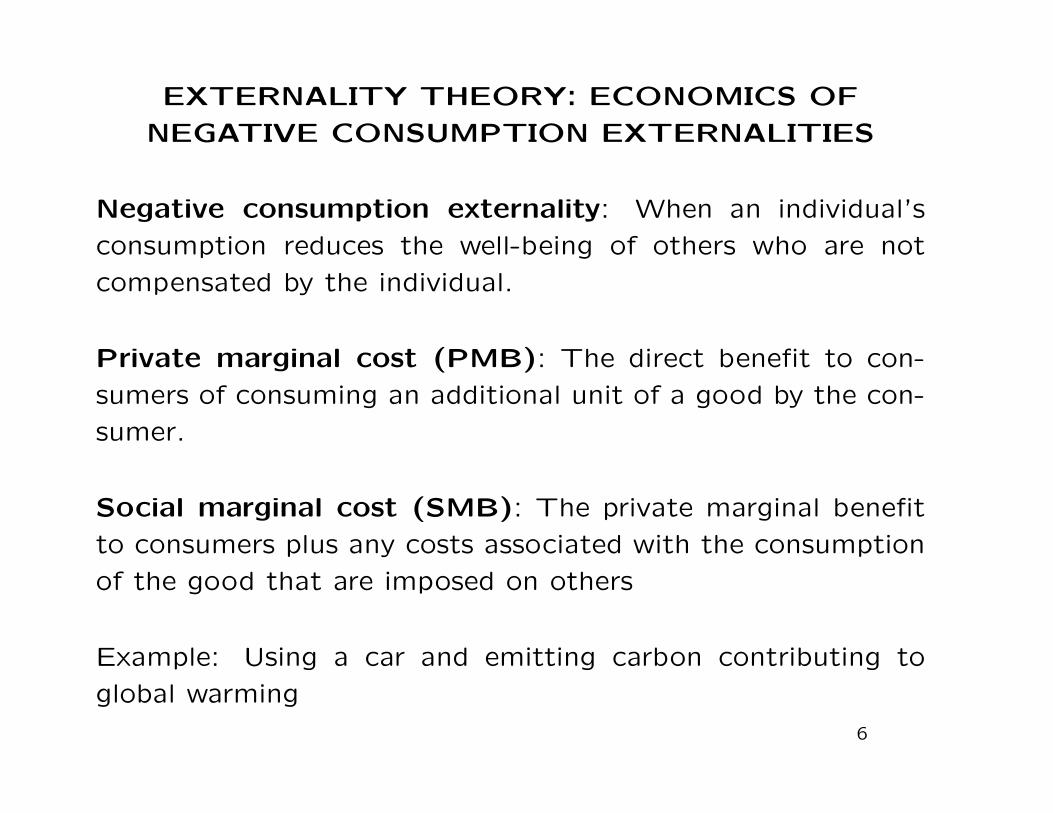
EXTERNALITY THEORY: ECONOMICS OF

NEGATIVE CONSUMPTION EXTERNALITIES

Negative consumption externality: When an individual’s

consumption reduces the well-being of others who are not

compensated by the individual.

Private marginal cost (PMB): The direct benefit to con-

sumers of consuming an additional unit of a good by the con-

sumer.

Social marginal cost (SMB): The private marginal benefit

to consumers plus any costs associated with the consumption

of the good that are imposed on others

Example: Using a car and emitting carbon contributing to

global warming

6

Public Finance and Public Policy Jonathan Gruber Fourth Edition Copyright © 2012 Worth Publishers 11 of 35

C H A P T E R 5 ■ E X T E R N A L I T I E S : P R O B L E M S A N D S O L U T I O N S

5.1

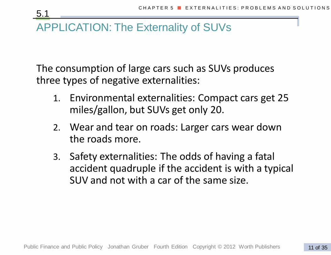
The consumption of large cars such as SUVs produces three types of negative externalities:

1. Environmental externalities: Compact cars get 25 miles/gallon, but SUVs get only 20.

2. Wear and tear on roads: Larger cars wear down the roads more.

3. Safety externalities: The odds of having a fatal accident quadruple if the accident is with a typical SUV and not with a car of the same size.

APPLICATION: The Externality of SUVs

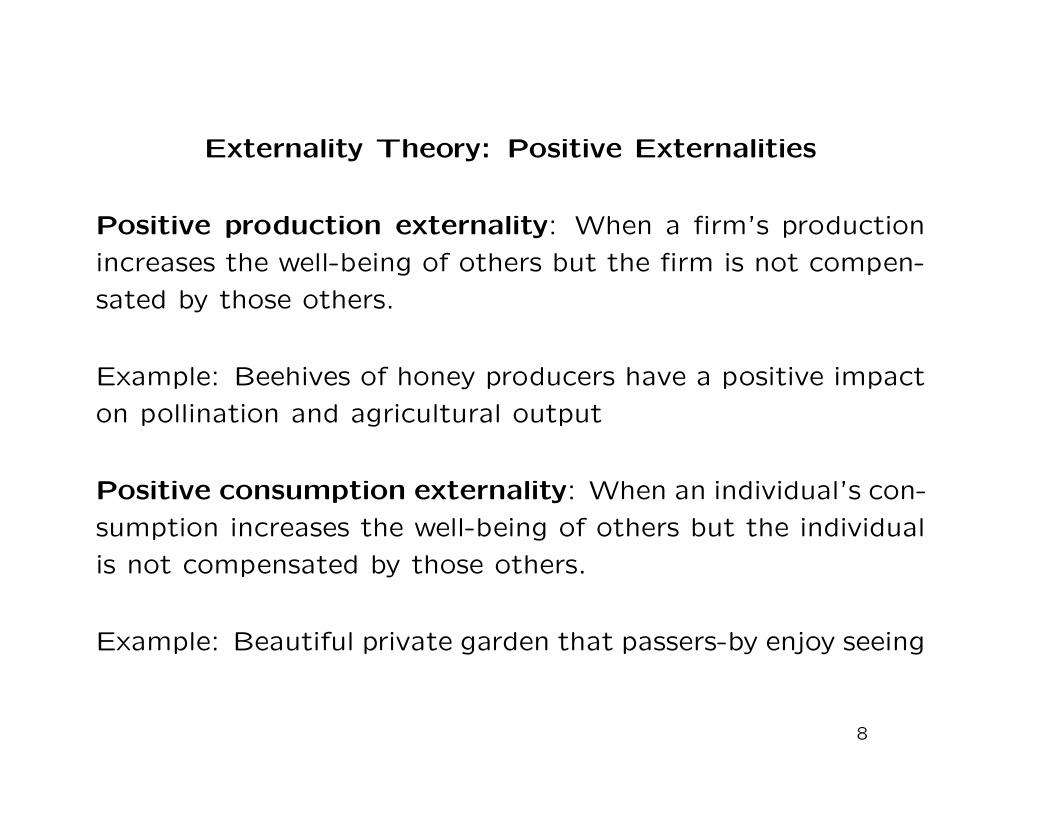
Externality Theory: Positive Externalities

Positive production externality: When a firm’s production

increases the well-being of others but the firm is not compen-

sated by those others.

Example: Beehives of honey producers have a positive impact

on pollination and agricultural output

Positive consumption externality: When an individual’s con-

sumption increases the well-being of others but the individual

is not compensated by those others.

Example: Beautiful private garden that passers-by enjoy seeing

8

Public Finance and Public Policy Jonathan Gruber Third Edition Copyright © 2010 Worth Publishers 13 of 34

C H A P T E R 5 ■ E X T E R N A L I T I E S : P R O B L E M S A N D S O L U T I O N S

Externality Theory 5.1

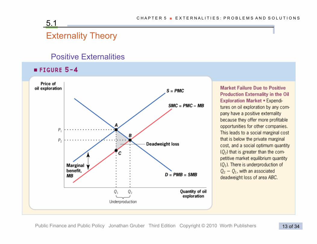
Positive Externalities

Externality Theory: Market Outcome is Inefficient

With a free market, quantity and price are such that PMB =

PMC

Social optimum is such that SMB = SMC

⇒ Private market leads to an inefficient outcome (1st welfare

theorem does not work)

Negative production externalities lead to over production

Positive production externalities lead to under production

Negative consumption externalities lead to over consumption

Positive consumption externalities lead to under consumption

10

Private-Sector Solutions to Negative Externalities

Key question raised by Ronald Coase (famous Nobel Prize

winner Chicago libertarian economist):

Are externalities really outside the market mechanism?

Internalizing the externality: When either private negotia-

tions or government action lead the price to the party to fully

reflect the external costs or benefits of that party’s actions.

11

PRIVATE-SECTOR SOLUTIONS TO NEGATIVE

EXTERNALITIES: COASE THEOREM

Coase Theorem (Part I): When there are well-defined prop-

erty rights and costless bargaining, then negotiations between

the party creating the externality and the party affected by

the externality can bring about the socially optimal market

quantity.

Coase Theorem (Part II): The efficient quantity for a good

producing an externality does not depend on which party is

assigned the property rights, as long as someone is assigned

those rights.

12

COASE THEOREM EXAMPLE

Firms pollute a river enjoyed by individuals. If firms ignore

individuals, there is too much pollution

1) Individuals own river: If river is owned by individuals then

individuals can charge firms for polluting the river. They will

charge firms the marginal damage (MD) per unit of pollution.

Why price pollution at MD? If price is above MD, individuals would wantto sell an extra unit of pollution, so price must rise. MD is the equilibriumefficient price in the newly created pollution market.

2) Firms own river: If river is owned by firms then firm can

charge individuals for polluting less. They will also charge

individuals the MD per unit of pollution reduction.

Final level of pollution will be the same in 1) and 2)

13

Public Finance and Public Policy Jonathan Gruber Fourth Edition Copyright © 2012 Worth Publishers 16 of 35

C H A P T E R 5 ■ E X T E R N A L I T I E S : P R O B L E M S A N D S O L U T I O N S

5.2

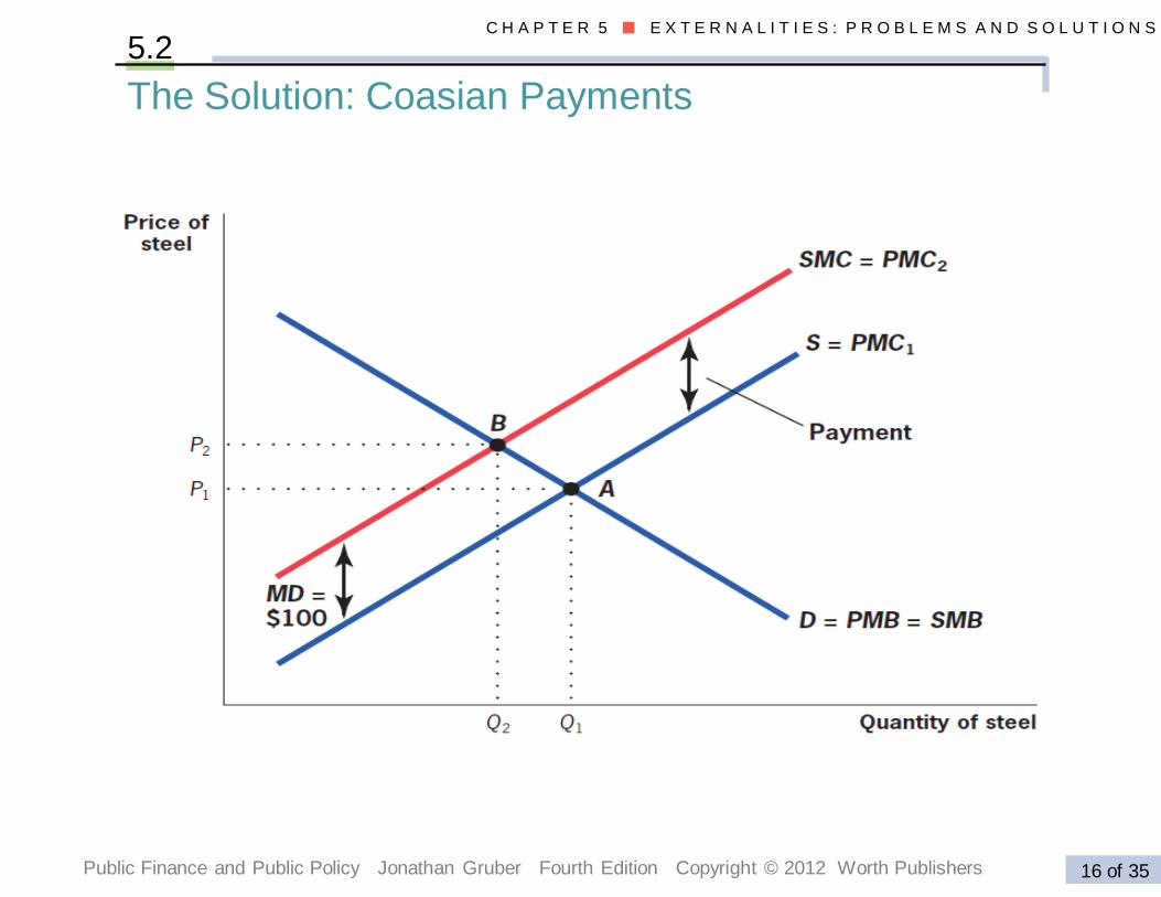
The Solution: Coasian Payments

PROBLEMS WITH COASIAN SOLUTION

In practice, the Coase theorem is unlikely to solve many of thetypes of externalities that cause market failures.

1) The assignment problem: In cases where externalitiesaffect many agents (e.g. global warming), assigning propertyrights is difficult

⇒ Coasian solutions are likely to be more effective for small, localized ex-

ternalities than for larger, more global externalities involving large number

of people and firms

2) The holdout problem: Shared ownership of propertyrights gives each owner power over all the others (becausejoint owners have to all agree to the Coasian solution)

As with the assignment problem, the holdout problem wouldbe amplified with an externality involving many parties.

15

PROBLEMS WITH COASIAN SOLUTION

3) Transaction Costs and Negotiating Problems: The

Coasian approach ignores the fundamental problem that it is

hard to negotiate when there are large numbers of individuals

on one or both sides of the negotiation.

This problem is amplified for an externality such as global

warming, where the potentially divergent interests of billions

of parties on one side must be somehow aggregated for a

negotiation.

16

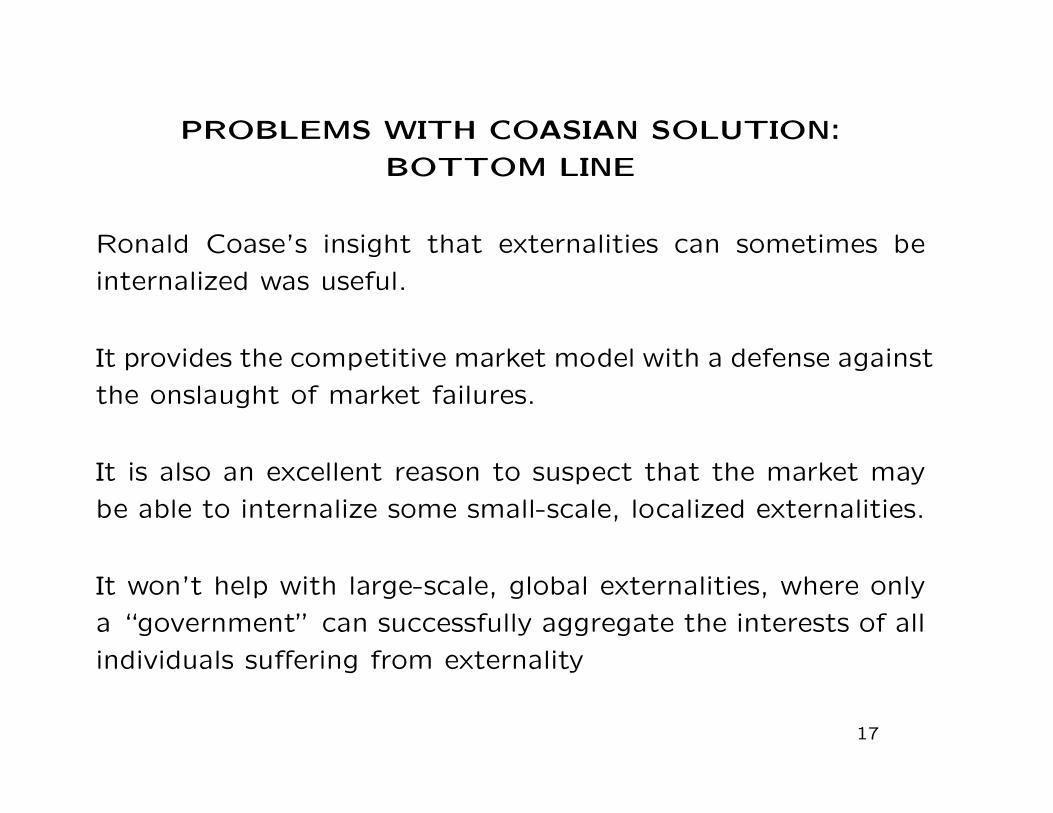
PROBLEMS WITH COASIAN SOLUTION:

BOTTOM LINE

Ronald Coase’s insight that externalities can sometimes be

internalized was useful.

It provides the competitive market model with a defense against

the onslaught of market failures.

It is also an excellent reason to suspect that the market may

be able to internalize some small-scale, localized externalities.

It won’t help with large-scale, global externalities, where only

a “government” can successfully aggregate the interests of all

individuals suffering from externality

17

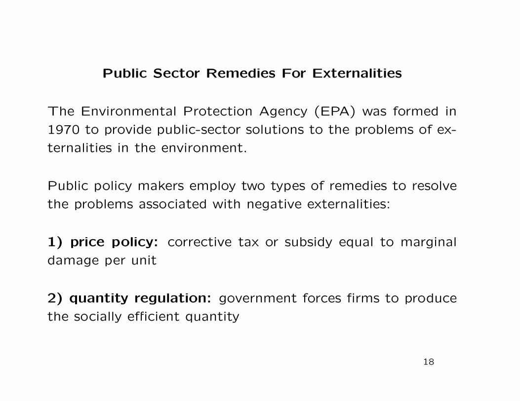
Public Sector Remedies For Externalities

The Environmental Protection Agency (EPA) was formed in

1970 to provide public-sector solutions to the problems of ex-

ternalities in the environment.

Public policy makers employ two types of remedies to resolve

the problems associated with negative externalities:

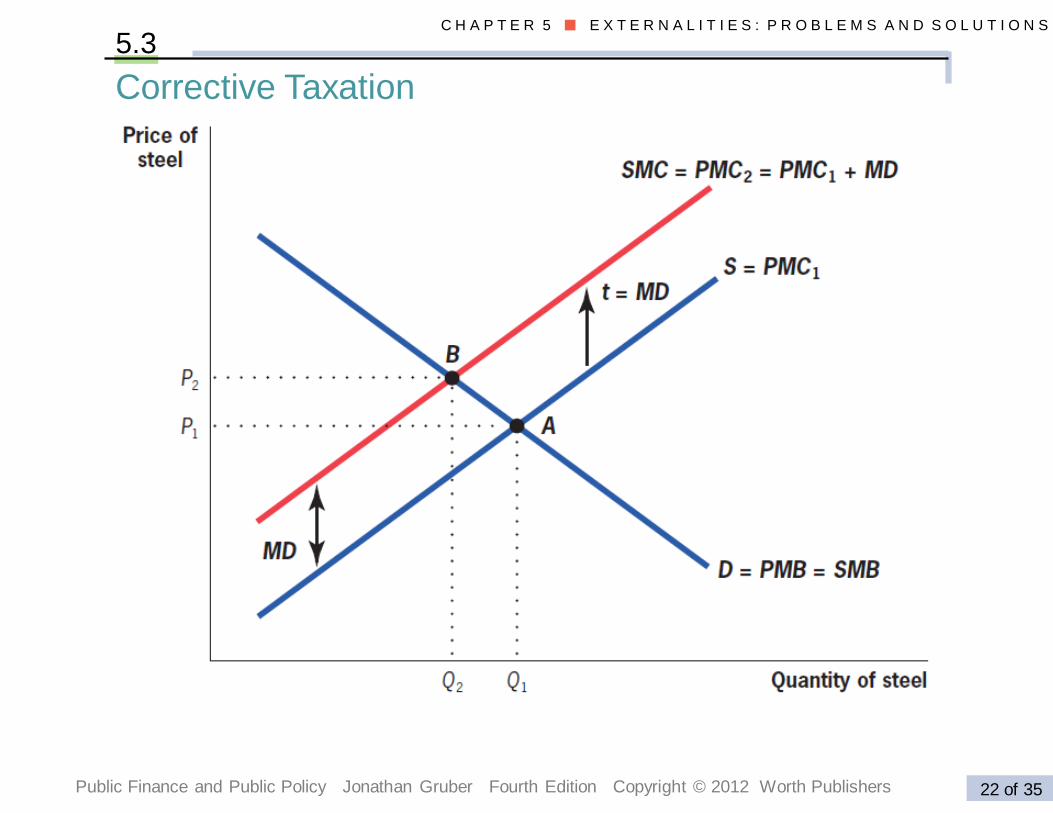
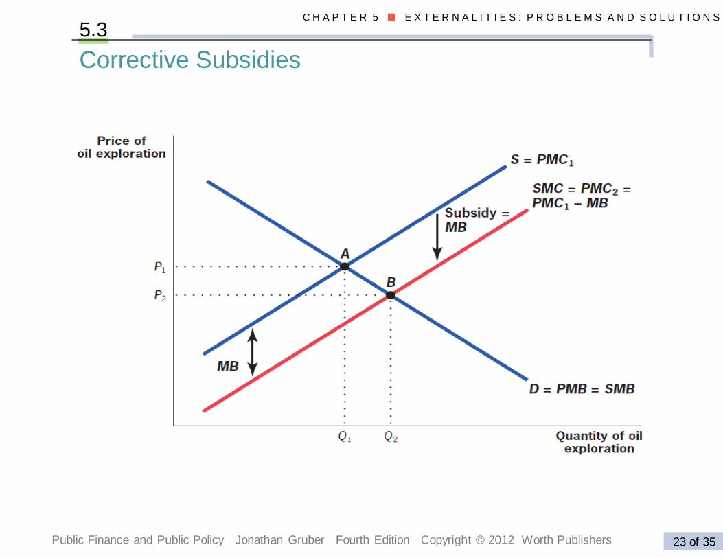
1) price policy: corrective tax or subsidy equal to marginal

damage per unit

2) quantity regulation: government forces firms to produce

the socially efficient quantity

18

Public Finance and Public Policy Jonathan Gruber Fourth Edition Copyright © 2012 Worth Publishers 22 of 35

C H A P T E R 5 ■ E X T E R N A L I T I E S : P R O B L E M S A N D S O L U T I O N S

5.3

Corrective Taxation

Public Finance and Public Policy Jonathan Gruber Fourth Edition Copyright © 2012 Worth Publishers 23 of 35

C H A P T E R 5 ■ E X T E R N A L I T I E S : P R O B L E M S A N D S O L U T I O N S

5.3

Corrective Subsidies

PUBLIC SECTOR REMEDIES FOR

EXTERNALITIES: REGULATION

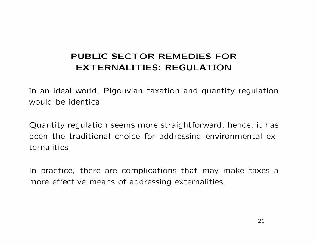
In an ideal world, Pigouvian taxation and quantity regulation

would be identical

Quantity regulation seems more straightforward, hence, it has

been the traditional choice for addressing environmental ex-

ternalities

In practice, there are complications that may make taxes a

more effective means of addressing externalities.

21

Public Finance and Public Policy Jonathan Gruber Fourth Edition Copyright © 2012 Worth Publishers 25 of 35

C H A P T E R 5 ■ E X T E R N A L I T I E S : P R O B L E M S A N D S O L U T I O N S

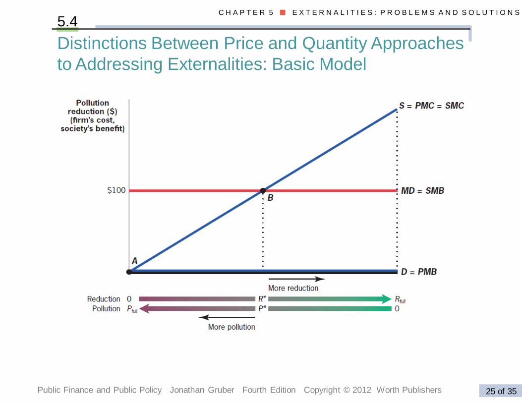
5.4

Distinctions Between Price and Quantity Approaches

to Addressing Externalities: Basic Model

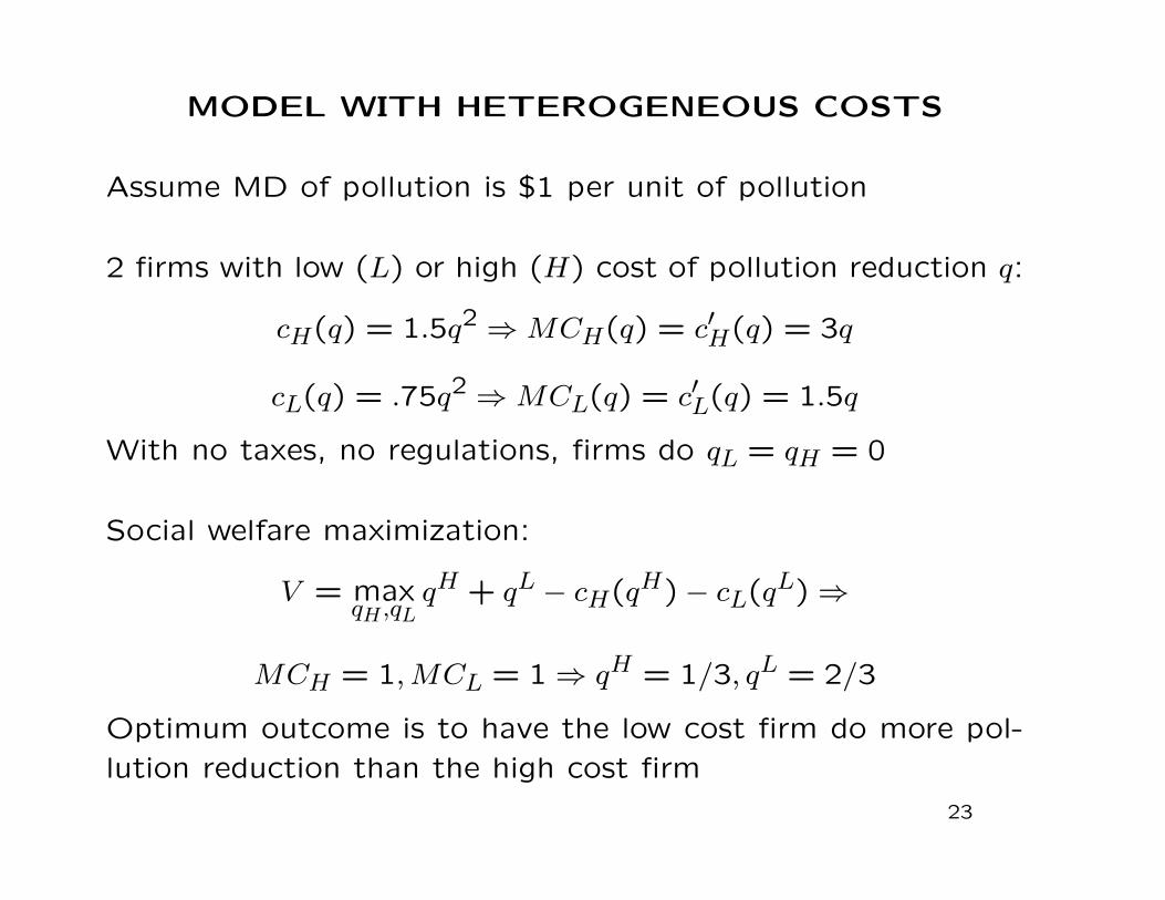
MODEL WITH HETEROGENEOUS COSTS

Assume MD of pollution is $1 per unit of pollution

2 firms with low (L) or high (H) cost of pollution reduction q:

cH(q) = 1.5q2 ⇒MCH(q) = c′H(q) = 3q

cL(q) = .75q2 ⇒MCL(q) = c′L(q) = 1.5q

With no taxes, no regulations, firms do qL = qH = 0

Social welfare maximization:

V = maxqH ,qL

qH + qL − cH(qH)− cL(qL)⇒

MCH = 1,MCL = 1⇒ qH = 1/3, qL = 2/3

Optimum outcome is to have the low cost firm do more pol-

lution reduction than the high cost firm

23

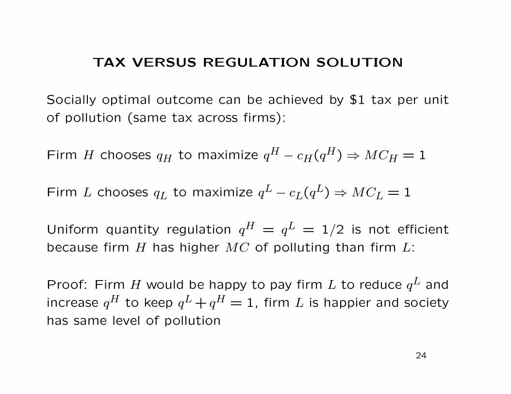
TAX VERSUS REGULATION SOLUTION

Socially optimal outcome can be achieved by $1 tax per unit

of pollution (same tax across firms):

Firm H chooses qH to maximize qH − cH(qH)⇒MCH = 1

Firm L chooses qL to maximize qL − cL(qL)⇒MCL = 1

Uniform quantity regulation qH = qL = 1/2 is not efficient

because firm H has higher MC of polluting than firm L:

Proof: Firm H would be happy to pay firm L to reduce qL and

increase qH to keep qL + qH = 1, firm L is happier and society

has same level of pollution

24

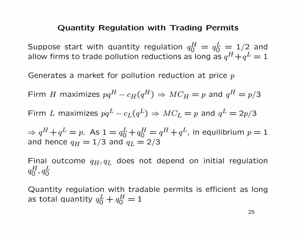
Quantity Regulation with Trading Permits

Suppose start with quantity regulation qH0 = qL0 = 1/2 andallow firms to trade pollution reductions as long as qH+qL = 1

Generates a market for pollution reduction at price p

Firm H maximizes pqH − cH(qH) ⇒ MCH = p and qH = p/3

Firm L maximizes pqL − cL(qL) ⇒ MCL = p and qL = 2p/3

⇒ qH +qL = p. As 1 = qL0 +qH0 = qH +qL, in equilibrium p = 1and hence qH = 1/3 and qL = 2/3

Final outcome qH , qL does not depend on initial regulationqH0 , qL0

Quantity regulation with tradable permits is efficient as longas total quantity qL0 + qH0 = 1

25

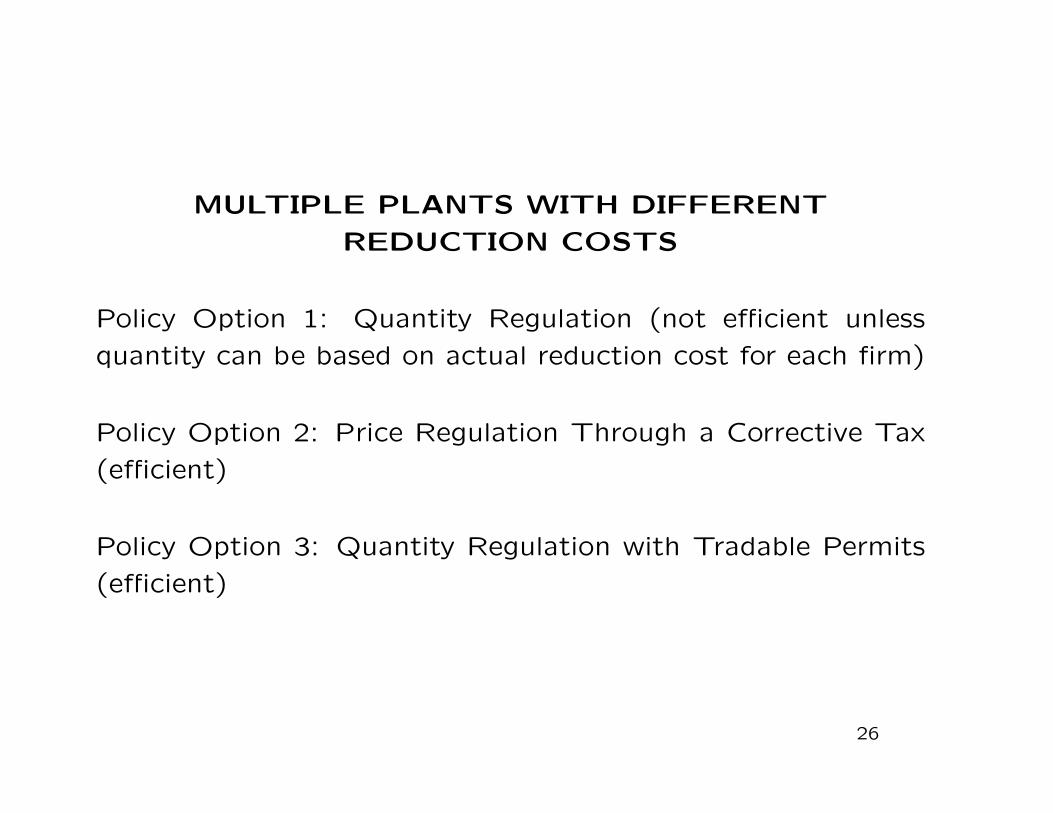
MULTIPLE PLANTS WITH DIFFERENT

REDUCTION COSTS

Policy Option 1: Quantity Regulation (not efficient unless

quantity can be based on actual reduction cost for each firm)

Policy Option 2: Price Regulation Through a Corrective Tax

(efficient)

Policy Option 3: Quantity Regulation with Tradable Permits

(efficient)

26

CORRECTIVE TAXES VS. TRADABLE PERMITS

Two differences between corrective taxes and tradable permits

(carbon tax vs. cap-and-trade in the case of CO2 emissions)

1) Initial allocation of permits: If the government sells them

to firms, this is equivalent to the tax

If the government gives them to current firms for free, this is

like the tax + large transfer to initial polluting firms.

2) Uncertainty in marginal costs: With uncertainty in costs

of reducing pollution, tax cannot target a specific quantity

while tradable permits can⇒ two policies no longer equivalent.

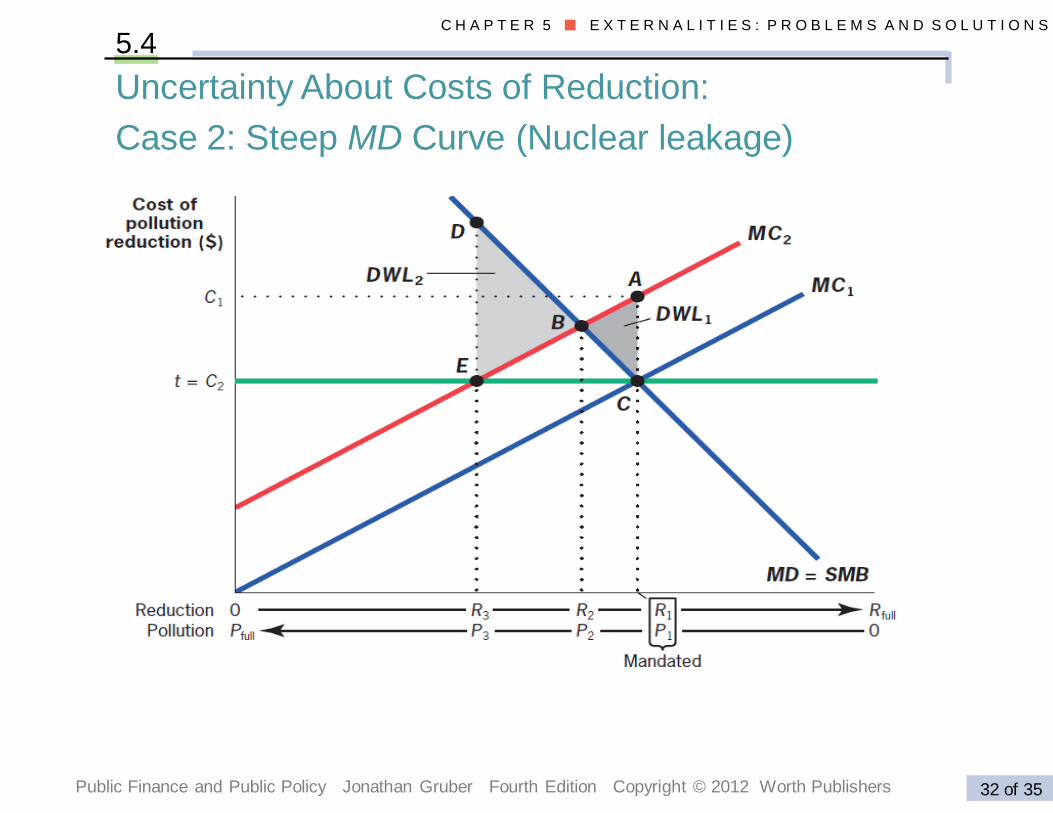
Taxes preferable when MD curve is flat. Tradable permits are

preferable when MD curve is steep.

27

Public Finance and Public Policy Jonathan Gruber Fourth Edition Copyright © 2012 Worth Publishers 31 of 35

C H A P T E R 5 ■ E X T E R N A L I T I E S : P R O B L E M S A N D S O L U T I O N S

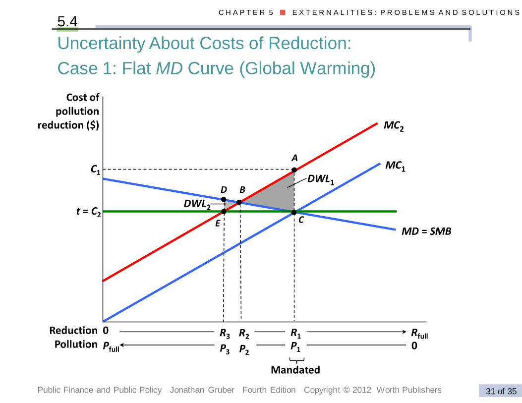
Uncertainty About Costs of Reduction:

Case 1: Flat MD Curve (Global Warming)

5.4

Cost of pollution

reduction ($)

MC1

MC2

MD = SMB

DWL1

DWL2

A

B

C

D

E

C1

t = C2

0ReductionPollution Pfull

Rfull

0

Mandated

P3 P2P1

R3 R2 R1

Public Finance and Public Policy Jonathan Gruber Fourth Edition Copyright © 2012 Worth Publishers 32 of 35

C H A P T E R 5 ■ E X T E R N A L I T I E S : P R O B L E M S A N D S O L U T I O N S

5.4

Uncertainty About Costs of Reduction:

Case 2: Steep MD Curve (Nuclear leakage)

Empirical Example: Acid Rain and Health

Acid rain due to contamination by emissions of sulfur dioxide

(SO2) and nitrogen oxide (NOx).

1970 Clean Air Act: Landmark federal legislation that first

regulated acid rain-causing emissions by setting maximum stan-

dards for atmospheric concentrations of various substances,

including SO2.

The 1990 Amendments and Emissions Trading:

SO2 allowance system: The feature of the 1990 amendments

to the Clean Air Act that granted plants permits to emit SO2

in limited quantities and allowed them to trade those permits.

29

Empirical Example: Effects of Clean Air Act of 1970

How does acid rain (or SO2) affect health?

Observational approach: relate mortality in a geographicalarea to the level of particulates (such as SO2) in the air

Problem: Areas with more particulates may differ from areaswith fewer particulates in many other ways, not just in theamount of particulates in the air

Chay and Greenstone (2003) use clean air act of 1970 toresolve the causality problem:

Areas with more particulates than threshold required to cleanup air [treatment group]. Areas with less particulates thanthreshold are control group.

Compares infant mortality across 2 types of places before andafter (DD approach)

30

Figure 2: Trends in TSPs Pollution and Infant Mortality, by 1972 Nonattainment Status

A. Trends in Mean TSPs Concentrations, by 1972 Nonattainment Status

50

60

70

80

90

100

110

1969 1970 1971 1972 1973 1974

Year

Mea

n of

Ave

rage

Dai

ly R

eadi

ngs

(Mic

rog

ram

s p

er C

ubic

Met

er)

Nonattainment Annual Mean Regulation Threshold Attainment

Source: Authors’ tabulations from EPA’s “Quick Look Reports” data file.

B. Trends in Internal Infant Mortality Rate, by 1972 Nonattainment Status

1400

1500

1600

1700

1800

1900

2000

2100

1969 1970 1971 1972 1973 1974

Year

Inte

rnal

Infa

nt M

orta

lity

Rat

e(p

er 1

00,0

00 L

ive

Bir

ths)

Nonattainment Attainment

Source: Chay and Greenstone (2003)

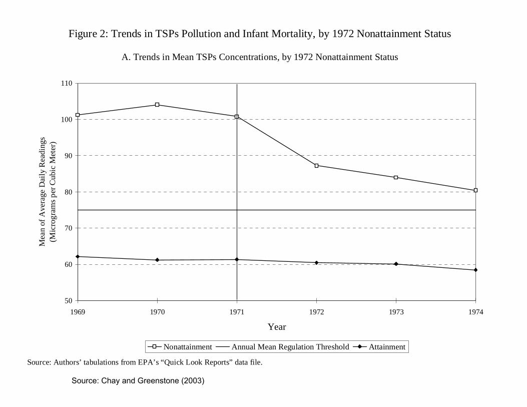
Figure 2: Trends in TSPs Pollution and Infant Mortality, by 1972 Nonattainment Status

A. Trends in Mean TSPs Concentrations, by 1972 Nonattainment Status

50

60

70

80

90

100

110

1969 1970 1971 1972 1973 1974

Year

Mea

n of

Ave

rage

Dai

ly R

eadi

ngs

(Mic

rog

ram

s p

er C

ubic

Met

er)

Nonattainment Annual Mean Regulation Threshold Attainment

Source: Authors’ tabulations from EPA’s “Quick Look Reports” data file.

B. Trends in Internal Infant Mortality Rate, by 1972 Nonattainment Status

1400

1500

1600

1700

1800

1900

2000

2100

1969 1970 1971 1972 1973 1974

Year

Inte

rnal

Infa

nt M

orta

lity

Rat

e(p

er 1

00,0

00 L

ive

Bir

ths)

Nonattainment Attainment

Source: Chay and Greenstone (2003)

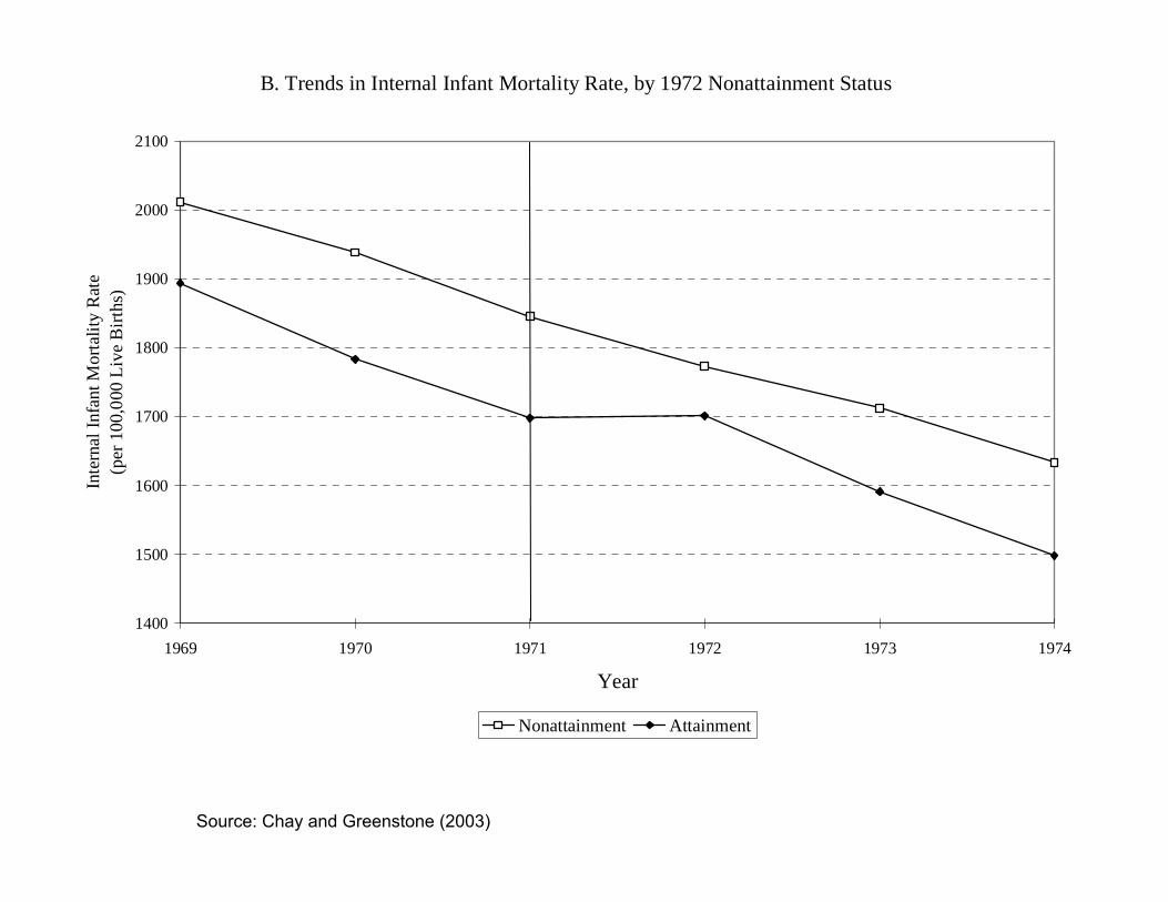
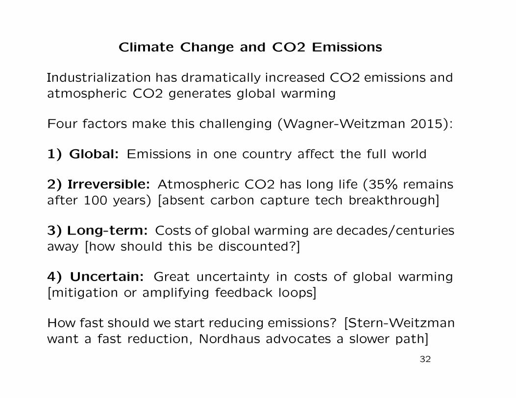
Climate Change and CO2 Emissions

Industrialization has dramatically increased CO2 emissions andatmospheric CO2 generates global warming

Four factors make this challenging (Wagner-Weitzman 2015):

1) Global: Emissions in one country affect the full world

2) Irreversible: Atmospheric CO2 has long life (35% remainsafter 100 years) [absent carbon capture tech breakthrough]

3) Long-term: Costs of global warming are decades/centuriesaway [how should this be discounted?]

4) Uncertain: Great uncertainty in costs of global warming[mitigation or amplifying feedback loops]

How fast should we start reducing emissions? [Stern-Weitzmanwant a fast reduction, Nordhaus advocates a slower path]

32

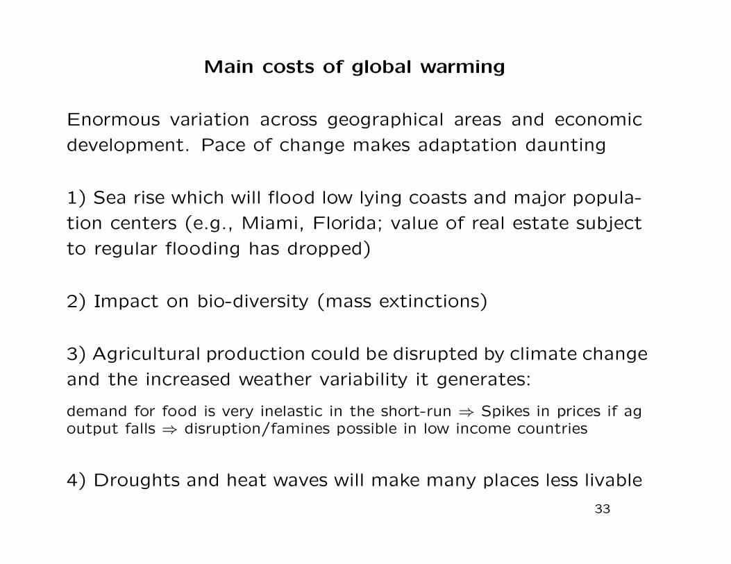
Main costs of global warming

Enormous variation across geographical areas and economic

development. Pace of change makes adaptation daunting

1) Sea rise which will flood low lying coasts and major popula-

tion centers (e.g., Miami, Florida; value of real estate subject

to regular flooding has dropped)

2) Impact on bio-diversity (mass extinctions)

3) Agricultural production could be disrupted by climate change

and the increased weather variability it generates:

demand for food is very inelastic in the short-run ⇒ Spikes in prices if agoutput falls ⇒ disruption/famines possible in low income countries

4) Droughts and heat waves will make many places less livable

33

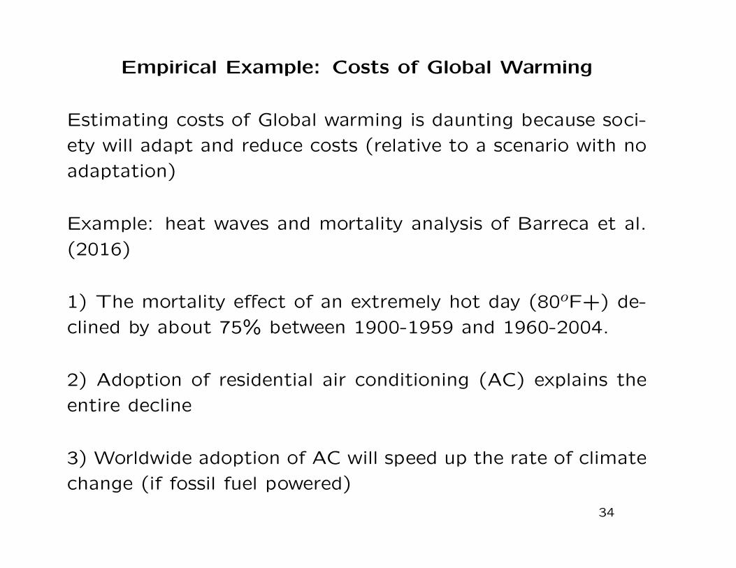
Empirical Example: Costs of Global Warming

Estimating costs of Global warming is daunting because soci-

ety will adapt and reduce costs (relative to a scenario with no

adaptation)

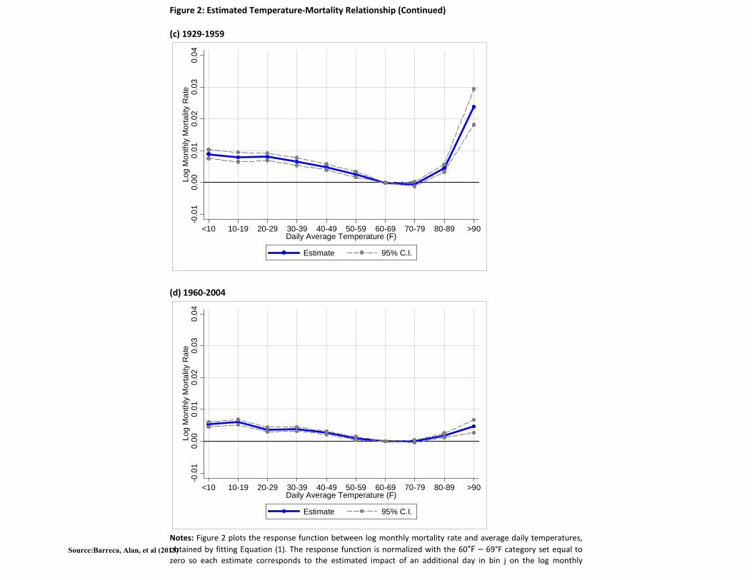
Example: heat waves and mortality analysis of Barreca et al.

(2016)

1) The mortality effect of an extremely hot day (80oF+) de-

clined by about 75% between 1900-1959 and 1960-2004.

2) Adoption of residential air conditioning (AC) explains the

entire decline

3) Worldwide adoption of AC will speed up the rate of climate

change (if fossil fuel powered)

34

32

Figure 2: Estimated Temperature-Mortality Relationship (Continued) (c) 1929-1959

(d) 1960-2004

Notes: Figure 2 plots the response function between log monthly mortality rate and average daily temperatures, obtained by fitting Equation (1). The response function is normalized with the 60°F – 69°F category set equal to zero so each estimate corresponds to the estimated impact of an additional day in bin j on the log monthly

-0.0

10

.00

0.0

10

.02

0.0

30

.04

Log

Mo

nth

ly M

ort

alit

y R

ate

<10 10-19 20-29 30-39 40-49 50-59 60-69 70-79 80-89 >90Daily Average Temperature (F)

Estimate 95% C.I.

-0.0

10

.00

0.0

10

.02

0.0

30

.04

Log

Mo

nth

ly M

ort

alit

y R

ate

<10 10-19 20-29 30-39 40-49 50-59 60-69 70-79 80-89 >90Daily Average Temperature (F)

Estimate 95% C.I.

Source:Barreca, Alan, et al (2013)

CURBING GLOBAL WARMING: KYOTO TREATY

Kyoto 1997: 35 industrialized nations (but not US) agreed

to reduce their emissions of greenhouse gases to 5% below

(depends on country) 1990 levels by the year 2012

Industrialized countries are allowed to trade emissions rights

among themselves, as long as the total emissions goals are

met [=quantity regulation with trading permits]

Developing countries are not in the treaty even though it is

cheaper to use fuel efficiently as you develop an industrial base

than it is to “retrofit” an existing industrial base

36

CURBING GLOBAL WARMING: FUTURE

In principle, reducing CO2 emissions could generate Paretoimprovement bc losers from global warming lose more in $than what emitters win from emitting

Challenge: in practice, remedies (such as carbon tax) createlosers who oppose change

Disagreement between rich and developing countries on whoshould bear the cost of curbing greenhouse gas emissions

In the US, Obama directed EPA to regulate CO2 emission[carbon tax or cap-and-trade requires congress law] but thiswill be undone under Trump

Higher price on carbon emissions [through taxes or tradingpermits] will be needed to curb emissions and global warming.Participation of the US and large devo countries (China, India)will be needed [Nordhaus 2013 and Wagner-Weitzman books]

37

REFERENCES

Jonathan Gruber, Public Finance and Public Policy, Fourth Edition, 2012Worth Publishers, Chapters 5 and 6

Barreca, Alan, et al. “Adapting to Climate Change: The Remarkable De-cline in the US Temperature-Mortality Relationship over the 20th Century.”Journal of Political Economy 124(1), 2016, 105-159.(web)

Chay, K. and M. Greenstone “Air Quality, Infant Mortality, and the CleanAir Act of 1970,”NBER Working Paper No. 10053, 2003.(web)

Ellerman, A. Denny, ed. “Markets for clean air: The US acid rain pro-gram.” Cambridge University Press, 2000.(web)

Gruber, Jonathan. “Tobacco at the crossroads: the past and future ofsmoking regulation in the United States.” The Journal of Economic Per-spectives 15.2 (2001): 193-212.(web)

Nordhaus, William D., and Joseph Boyer. “Warning the World: EconomicModels of Global Warming.” MIT Press (MA), 2000.(web)

Nordhaus, William D. “After Kyoto: Alternative mechanisms to controlglobal warming.” The American Economic Review 96.2 (2006): 31-34.(web)

38

Nordhaus, William D. The Climate Casino: Risk, Uncertainty, and Eco-nomics for a Warming World, Yale University Press, 2013.

Wagner, Gernot and Martin L. Weitzman. Climate Shock: The Economic

Consequences of a Hotter Planet. Princeton University Press 2015.