1

November 6, 2006

M. Schinnerl, M. Kaltenbacher, U. Langer, R. Lerch, J. Schoberl

An Efficient Method for the Numerical Simulation of Magneto-MechanicalSensors and Actuators

The dynamic behavior of magneto-mechanical sensors and actuators can be completely described by Maxwell’s andNavier-Lame’s partial differential equations (PDEs) with appropriate coupling terms reflecting the interactions ofthese fields and with the corresponding initial, boundary and interface conditions. Neglecting the displacement cur-rents, which can be done for the classes of problems considered in this paper, and introducing the vector potentialfor the magnetic field, we arrive at a system of degenerate parabolic PDEs for the vector potential coupled with thehyperbolic PDEs for the displacements. Usually the computational domain, the finite element discretization, the timeintegration, and the solver are different for the magnetic and mechanical parts. For instance, the vector potentialis approximated by edge elements whereas the finite element discretization of the displacements is based on nodalelements on different meshes. The most time consuming modules in the solution procedure are the solvers for both,the magnetical and the mechanical finite element equations arising at each step of the time integration procedure.We use geometrical multigrid solvers which are different for both parts. These multigrid solvers enable us to solvequite efficiently not only academic test problems, but also transient 3D technical magneto-mechanical systems of highcomplexity such as solenoid valves and electro-magnetic-acoustic transducers. The results of the computer simulationare in very good agreement with the experimental data.

1 Introduction

Magneto-mechanical sensors and actuators are used in various technical devices. For instance as force-sensors andvalve-actuators in automatization-engineering, in injection-valves for diesel engines or as actuators in loudspeakers.The numerical simulation is an important tool for designing and optimizing these sensors and actuators.

The basis for the numerical simulation is a mathematical model that describes the dynamic behavior of magneto-mechanical sensors and actuators. Such kind of magneto-mechanical systems can be modeled by Maxwell’s andNavier-Lame’s partial differential equations (PDEs) describing the electromagnetic field and the mechanical field,respectively. The interaction of these fields is taken into account by additional terms in the PDE systems. Themathematical model is completed by appropriate initial, boundary and interface conditions. Neglecting the displace-ment currents, which can be done for a wide range of sensor and actuators, and introducing the vector potential forthe magnetic field, we arrive at a system of degenerate parabolic PDEs for the vector potential coupled with thehyperbolic PDEs for the displacements.

The line variational formulations (called sometimes also weak formulations) of the PDE systems are the startingpoint for the finite element discretization. The mechanical displacements, which are living in H1, are approximatedby nodal tedrahedrial finite elements, whereas the vector potential, which is living in H(curl), is discretized byedge tedrahedrial finite elements. We notice that the edge finite element discretization ensures the continuity of thetangential component of vector potential. We use different meshes for approximating the mechanical displacementsand the magnetic vector potential. These meshes are obtained from different refinement strategies of a commoncoarse mesh that represents the geometry. Special transfer operators manage the transfer of magnetic quantitiesfrom the magnetic grids to the mechanical grids and vice versa. These transfers are needed in the coupling terms.

This finite element discretization results in a large-scale second-order ordinary differential equation (ODE) systemfor the nodal values of the displacements that is strongly coupled with a large-scale first-order ODE system for theedge degrees of freedoms (dofs) determining the finite element approximation to the magnetic vector potential. Thesecond-order ODE system is numerically integrated by a Newmark scheme, whereas the first-order ODE systemis solved by generalized trapezoidal rule. The time integration is connected with some coupling iteration takinginto account the coupling of the ODE systems in a weak way. Since the time integration schemes are implicit, wehave to solve a large-scale linear mechanical system and a large-scale non-linear magnetic system at each step. Thenon-linearity in the magnetic system is due to the dependence of the permeability on the induction in ferromagnetic

2 2 PARTIAL DIFFERENTIAL EQUATIONS FOR THE MAGNETIC AND THE MECHANICAL FIELDS

materials. The non-linear magnetic system is solved by a fixed point iteration combined with some line-searchalgorithm. Finally, in both cases the arising linear systems are solved by special designed multigrid methods. Themultigrid method for the mechanical system uses a block Gauss-Seidel smoother that takes into account the strongcoupling of nodal displacements belonging to one node, whereas the multigrid method for the magnetic systems usesthe special block smoothers proposed in [1]. An alternative multigrid technique for Maxwell’s equations was proposedin [14]. The solution of these linear systems of finite element equations is certainly the most time-consuming part ofthe whole numerical algorithms. Thanks to the efficiency of these multigrid methods we can successfully solve notonly academic test problems, but also transient 3D technical magneto-mechanical systems of high complexity suchas magnetic valves and electro-magnetic-acoustic transducers.

To the best knowledge of the authors, there is neither a complete mathematical analysis of the coupled magneto-mechanical model discussed in this paper nor a complete numerical analysis of the complicated numerical algorithmpresented in this paper. Therefore, in order to verify the mathematical model and the accuracy of the numericalalgorithm proposed, we perform a lot of numerical simulations for real-life problem containing all difficulties whichare characteristic for industrial applications and compare the numerical results with the measurements made alongwith the numerical simulations. The first test example is a solenoid valve. We create a finite element model for thecomputer simulation and, at the same time, we build the same solenoid valve for real experiments and measurements.Due to the construction of the valve, a full 3-D simulation of the model must be performed. Additionally, the usedmaterial is strongly nonlinear and the movement of the armature causes a displacement of the FE-mesh. Also thevery low penetration-depth of the magnetic-field is a challenge for the numerical simulation.An electro-magnetic-acoustic transducer (EMAT) serves as a second example. The EMAT can be considered as a3D linear problem, because the used materials are linear and the mechanical displacements are small. Nevertheless,the dimensions of the EMAT, which are very large in comparison to the small penetration depth of the magneticfield, cause a very high number of 3D finite elements. Therefore, only 2-D simulations of EMATs were performed inthe past [26].

The remaining part of the paper is organized as follows. In Section 2, we present the PDEs describing the transientbehavior of the mechanical and magnetical fields, together with the appropriate initial, boundary, and interfaceconditions. Special emphasis is given to the discussion of the influence of the coupling terms. Section 3 introducesthe variational line formulations of both field problems which are the starting point for the finite element semidis-cretization. The time integration, the iterative coupling, and the multigrid handling are discussed in Section 4. Thecoupling of the magnetic system to an electrical network with a given voltage and its handling in our numericalscheme is also discussed in Sections 3 and 4, respectively. Section 5 deals with the computer simulation of two real-life applications and their verification by experimental results. Finally, in the last section, we give some concludingremarks.

2 Partial Differential Equations for the Magnetic and the MechanicalFields

In this section, we briefly present the Navier-Lame and the Maxwell PDE systems describing the dynamic mechanicalbehavior and the transient electromagnetic behavior of magneto-mechanical sensors and actuators, respectively. Theeddy current approximation to Maxwell’s equations is appropriate for our class of problems. We put special emphasison the terms modeling the coupling of mechanical and magnetical fields. The describing equations are completed byappropriate initial, boundary and, interface conditions.

2.1 The Mechanical System

If geometrically linear elasticity and isotropic linear material are assumed, the dynamical behavior of mechanicalsystems can be modeled by the Navier-Lame PDE system

ρ∂2~d

∂t2+ c

∂ ~d

∂t− E

2(1 + ν)

(

(∇ · ∇)~d +1

1 − 2ν∇(∇ · ~d)

)

= ~fV , (1)

2.2 The Magnetic System and the Coupling Terms 3

where ~fV denotes the volume forces, E Young’s modulus, ν the Poisson ratio, ρ the specific density and c aviscous damping of the material. On the boundary Γmech of the mechanical computational domain Ωmech either themechanical displacements ~d (Dirichlet boundary) or the mechanical normal stresses ~σn (Neumann boundary) or amechanical impedance are given [38]. On interfaces, the continuity of the displacements and the normal stresses is

required. The initial conditions prescribed for the displacements ~d and the velocities ∂ ~d/∂t complete the mechanicalequations.

2.2 The Magnetic System and the Coupling Terms

The transient electromagnetic behavior of magneto-mechanical sensors and actuators is described by Maxwell’sequations, see e.g. [37]. Neglecting high frequency displacement currents, that can be always done without restrictionsfor the considered class of problems, we can rewrite Maxwell’s equations in the form

∇× ~H = ~J (Ampere’s law), (2)

∇× ~Es = −∂ ~B

∂t(Faraday’s law), (3)

∇ · ~B = 0 . (4)

In equations (2) - (4) ~H denotes the magnetic field strength, ~J the electric current density, ~B the magnetic induction

and ~Es the solenoidal part of the electric field ~E, which computes as

~E = ~Ee + ~Es (5)

with ~Ee the irrotational part of ~E. These equations must be completed by the constitutive relations

~B = µ ~H, (6)

~J = ~Je + γ(

~Es + ~v × ~B)

, (7)

where ~v is the velocity, γ the specific electrical conductivity and µ the permeability of the material. ~Je = γ ~Ee

denotes a given current density. We mention that in ferromagnetic materials the permeability depends on themagnetic induction.

The physical quantities ~H, ~B and ~J have to fulfill not only equations (2) - (7) but also certain interface- andboundary-conditions. In Fig.1 an eddy-current problem is shown. The regions Ω1 and Ω2 consist of materials with

eddy currents

no eddy currents

Figure 1: Model of an eddy-current problem.

the conductivities γ1 and γ2. In Ω1 and Ω2 eddy currents can arise. The region Ω3 has no conductivity but possibly

4 2 PARTIAL DIFFERENTIAL EQUATIONS FOR THE MAGNETIC AND THE MECHANICAL FIELDS

an impressed current ~Je. The boundary Γ = ∂Ω of the whole domain Ω = Ω1 ∪Ω2 ∪Ω3 usually consists of the partsΓH and ΓB with the boundary conditions

~B · ~n = 0 on ΓB (8)

and

~H × ~n = ~K on ΓH . (9)

In equations (8) and (9) ~n denotes the outer normal unit-vector to the boundary Γ. ~K is a given surface current-density. On the interface Γ12 between Ω1 and Ω2 the interface conditions

~B1 · ~n1 + ~B2 · ~n2 = 0,~H1 × ~n1 + ~H2 × ~n2 = 0

on Γ12 (10)

(11)

must hold. The normal unit-vectors are oriented in opposite direction which means that

~n2 = −~n1. (12)

Furthermore, since the the current ~J is divergence-free, the condition

~J1 · ~n1 + ~J2 · ~n2 = 0 (13)

must hold on Γ12, too. On the boundaries Γ13 and Γ23, analogous conditions must be valid.

Introducing a magnetic vector potential ~A

~B = ∇× ~A (14)

leads according to equation (3) to the relation

~Es = −∂ ~A

∂t, (15)

so that we can transfer equations (2)-(7) to the form

γ∂ ~A

∂t+ ∇× (

1

µ∇× ~A) + −γ~v × (∇× ~A) = ~Je . (16)

For large Peclet-numbers

Pe =µγvh

2>> 1, (17)

the term γ~v × (∇ × ~A) becomes dominant and causes instabilities in the numerical solution process [24]. In (17),h denotes the discretization parameter in direction of the velocity ~v. However, if due to mechanical movements /deformations the overall magnetic field is changed (e.g., movement of the armature in a magnetic valve), we haveto consider the formulation of the magnetic problem on the deformed geometry [24]. Observing some point P ina fixed reference frame Γ(x, y, z) (see Fig. 2), we can express the spatial and temporal variation of the magnetic

vector potential ~A at this point by the formula

∆ ~A

∆t=

~A(~d + ∆~d, t + ∆t) − ~A(~d, t)

∆t

=~A(~d + ∆~d, t + ∆t) − ~A(~d, t + ∆t)

∆t+

~A(~d, t + ∆t) − ~A(~d, t)

∆t.

2.2 The Magnetic System and the Coupling Terms 5

Figure 2: Movement of a considered point P.

For ∆t → 0, the expression (18) leads to the relation

d ~A

dt=

∂ ~A

∂t+ (~v · ∇) ~A. (18)

On the other hand, the electromotive force can be rewritten as1

~v × (∇× ~A) = ∇ ~A(~v · ~A) − (~v · ∇) ~A. (19)

Using (18) and (19), we can transform the partial differential equation (16) into the form

γd ~A

dt+ ∇× (

1

µ∇× ~A) − γ∇ ~A

(~v · ~A) = ~Je . (20)

Equation (20) illustrates, that the total differential d ~A/dt takes the induced current caused by the electromotive

force implicitly into account, but in return the term γ∇ ~A(~v · ~A) must be considered additionally. If ~v and ~A are

orthogonal, this term disappears, which is the case for all 2D problems. Besides the electromotive force, also magneticforces cause a coupling between the magnetic and the mechanical field. The magnetic volume-force, produced bythe magnetic field, can be separated into two parts. The first effect is the Lorentz-force,

~fV,L = ~J × ~B, (21)

which occurs when a magnetic induction ~B exists in a body with a current-density ~J . Using the magnetic vectorpotential ~A, (21) can be rewritten as

~fV,L =

(

~Je − γdA

dt+ γ∇ ~A

(~v · ~A)

)

× (∇× ~A). (22)

In the case of non-constant permeability, especially in the presence of ferromagnetic materials, an additional force

~fV,µ = −1

2

∣

∣

∣

∣

1

µ∇× ~A

∣

∣

∣

∣

2

∇µ (23)

arises. At an interface between two materials with the permeabilities µ1 and µ2, the volume-force formulation (23)can be transferred into Maxwell’s surface force-density formulation [37]

~fΓ = (~n · ~H) ~B − ~n1

2~B · ~H. (24)

1∇ ~A(~v · ~A) means, that the gradient is used only for the terms of the magnetic vector potential ~A.

6 3 VARIATIONAL FORMULATION AND FINITE ELEMENT DISCRETIZATION

Material 1Material 2

Figure 3: Interface between two materials with different permeabilities.

This formulation can also be written with the help of a tensor [T ], which allows the calculation of the magnetic forceand moment acting to a body by the equations (see [36], pp. 154–155, and [18])

~F =

∮

~A

[T ] d ~A (25)

and

~M =

∮

~A

~r × ([T ] d ~A). (26)

We mention that (24) must not consider the jump of the magnetic permeability at the interface of the ferromagneticmaterial. So it is sufficient to calculate (24) only at the finite elements of the non-ferromagnetic domain which areconnected to the interface.For problems with permanent-magnetic materials the additional force term

~fV 3 = − ~H ∇ · ~M (27)

must be considered. ~M is the magnetization of the used permanent magnetic material. At last the magnetostrictioncoupling effect is described by

~fV 4 =

H∫

0

∇(

| ~H |2ρ∂µ

∂ρ

)

d ~H, (28)

where ρ denotes the specific density. Magnetostrictive actuators are especially suited for the generation of highforces. But this effect is not covered here.

3 Variational Formulation and Finite Element Discretization

This section provides the variational formulations of the mechanical and magnetic PDE systems which are, of course,coupled. The coupled variational formulations are the starting point for the finite element semi-discretization thatresults into a second-order mechnical ODE system and a first-order magnetic ODE system which are again coupled.Finally, we describe a magnetic system that is coupled to an electrical network with an impressed voltage.

3.1 Mechanical System 7

3.1 Mechanical System

By multiplying the mechanical differential equation (1) with a weighting function ~w and integrating over the domainΩmech, the mechanical problem is transferred to the weak form

∫

Ω

(

ρ∂2 ~d

∂t2+ c

∂ ~d

∂t− E

2(1 + ν)

(

(∇ · ∇)~d +1

1 − 2ν∇(∇ · ~d)

)

)

· ~w dΩ =

∫

Ω

~fV · ~w dΩ. (29)

Using Green’s first identity and the symmetry of the stress tensor, we obtain the variational formulation or theso-called weak form [16]

∫

Ωmech

ρ∂2di

∂t2widΩ +

∫

Ωmech

~ǫ(~d)T D~ǫ(~w)dΩ +

∫

Ωmech

c∂di

∂twidΩ =

∫

Ωmech

fiwidΩ +

∫

Γni

σniwidΓ (30)

of (1), see e.g. [16]. In (30), i denotes the spatial direction (x, y or z), ~ǫ the components of the mechanical straintensor in Voigt notation, D the tensor of the elastic coefficients, and Γni the boundary with given surface stress σni.The mechanical domain is now discretized with the help of nodal finite elements. Thereby, the mechanical displace-ments are approximated in the form

~d ≈nn∑

k=1

Nk~dk, (31)

where Nk denotes the shape function of the k-th node, ~dk the displacement at the k-th node and nn the numberof nodes. By using (31) in (30) and applying Galerkin’s technique, the system of second-order ordinary differentialequations (ODE)

M∂2d

∂t2 + C∂d

∂t + Kd = F (32)

is obtained, where the mass matrix M, the stiffness matrix K and the force vector F have the following form:

• mass matrix:

M = [Mab]

Mab = δij

∫

Ω

NaρNb dΩ (33)

1 ≤ a, b ≤ neq

1 ≤ i, j ≤ nsd

• stiffness matrix:

K = [Kab]

Kab = ~eTi

∫

Ω

BTa DBb dΩ~ej (34)

1 ≤ a, b ≤ neq

1 ≤ i, j ≤ nsd

8 3 VARIATIONAL FORMULATION AND FINITE ELEMENT DISCRETIZATION

in the 3D case:

Ba =

∂Na

∂x0 0

0 ∂Na

∂y0

0 0 ∂Na

∂z

0 ∂Na

∂z∂Na

∂y∂Na

∂z0 ∂Na

∂x∂Na

∂y∂Na

∂x0

(35)

• force vector:

F = Fa

Fa =

∫

Ω

NafidΩ +

∫

Γni

NaσnidΓ (36)

In (33) - (36) neq denotes the number of unknowns, ~ei the unity vector in the spatial direction i, δij Kronecker’soperator and nsd the spatial dimension of the mechanical field. The damping matrix C is chosen as a linearcombination of M and K [5], i.e.

C = αM + βK. (37)

The magnitudes of the Rayleigh coefficients α and β depend on the energy dissipation characteristics of the modeledmechanical problem.

3.2 Magnetic System

By multiplying the magnetic system (20) with a weighting function ~W , integrating over the domain Ωmag(~d), which

is deformed by the mechanical displacement ~d, and applying the first Green’s identity, the magnetic field can beexpressed in a weak sense by the variational formulation

∫

Ωmag

γd ~A

dt· ~W dΩ +

∫

Ωmag

1

µ(∇× ~A) · (∇× ~W ) dΩ −

∫

Ωmag

γ ∇ ~A(~v · ~A) · ~W dΩ =

∫

Ωmag

~Je · ~W dΩ +

∫

Γmag,H

( ~H × ~n) · ~W dΓ, (38)

where Γmag,H denotes a boundary with specified ~H × ~n. In order to achieve an appropriate FE-discretization of

x

yz

interface G n

11

22

material 1 (m ,g )

material 2 (m , g )

Figure 4: Interface between two materials.

the magnetic system, the properties of the magnetic field at an interface must be analyzed in a more detailed way.In Fig. 4 an interface between two materials with the permeabilities µ1 and µ2 and the conductivities γ1 and γ2 is

3.2 Magnetic System 9

displayed. For simplicity and without loos of generality, the interface lies in the x-y plane and the normal-vector ~nis exactly oriented in z-direction. Using (14) and (10), the condition

Bn = Bz =∂Ay1

∂x− ∂Ax1

∂y=

∂Ay2

∂x− ∂Ax2

∂y(39)

must be fulfilled. Equation (39) can be enforced explicitly, if the tangential component of ~A is continuous at theinterface. As mentioned in sect. 2.2 displacement currents are neglected, which enables the reformulation of (13) onan interface between two eddy-current regions as

~n · γ1∂A1

∂t= ~n · γ2

∂A2

∂t. (40)

Therefore, in z direction, equation

∂

∂t[γ1Az1 − γ2Az2] = 0 (41)

must hold. As the magnetic vector potential is not static, (41) requires discontinuity of Az if γ1 6= γ2. For nodalfinite elements one needs a splitting of the magnetic vector potential in a new vector, which has to be divergencefree, and a gradient of a scalar potential (corresponds to a decomposition of the space H(curl)). In addition, aweighted regularization according to [7] has to be applied. For a detailed discussion we refer to [19]. The “natural”choice of the spatial discretization are edge-finite-elements [28]. Thereby, the degrees of freedom are not attached tothe element nodes, but to the element edges. In Fig. 5 a linear edge-tetrahedron-element is shown. Using the edge

4

A5

A3

A6

3

2

1

A

A

A

1

4

2

Figure 5: Linear edge tetrahedron.

element discretization, the magnetic vector field ~A is approximated by

~A ≈nk∑

k=1

~NkAk. (42)

In (42), ~Nk denotes the vectorial shape function, which is associated with the k-th edge ek, nk the number of edgesin the magnetic FE mesh, and

Ak =

∫

ek

~A · d~s (43)

approximates the line-integral over the projection of the magnetic vector potential ~A to the k-th edge ek. Inserting(42) into the weak formulation (38) leads to the first-order ODE system

L

dA

d t

+ PA + P2(~v)A = Q. (44)

The conductivity matrix L, the permeability matrix P, the second permeability matrix P2 and the source vectorQ have the form:

10 3 VARIATIONAL FORMULATION AND FINITE ELEMENT DISCRETIZATION

• conductivity matrix:

L = [Lab]

Lab =

∫

Ωmag(~d)

~Na · γ ~NbdΩ (45)

1 ≤ a, b ≤ nk

• permeability matrix:

P = [Pab]

Pab =

∫

Ωmag(~d)

(1

µ∇× ~Na) · (∇× ~Nb) dΩ (46)

1 ≤ a, b ≤ nk

• permeability matrix 2:

P2 = [P2ab]

P2ab = −∫

Ωmag(~d)

γ∇ ~A(~v · ~Na) · ~Nb dΩ (47)

1 ≤ a, b ≤ nk

• source vector:

Q = Qb

Qb =

∫

Ωmag(~d)

~Na · ~Je dΩ (48)

1 ≤ b ≤ nk

Here, the boundary integral term in (38) is assumed to be zero.The solution of (44) requires special care in order to obtain an optimal solver. We suggest to add a fictive electricconductivity γ′ to regions with zero electric conductivity to obtain a variational form, which is H(curl)-elliptic. Ofcourse, this fictive conductivity γ′ has to be chosen small as compared to the reluctivity of the material. The proofof convergence even in the case of γ′ → 0 is given in [30] and [3] for the magnetostatic case and for the eddy currentcase, respectively.

3.3 Voltage Loading

Frequently the magnetic system (20) is not excited by a given current density ~Je, but is coupled to an electricalnetwork with a given voltage U . In Fig. 6, the simplest case of an electrical network, consisting of the coil resistorRcoil placed in series with the FE-model is shown. Thereby, not only the magnetic vector potential ~A, but also thecurrent I is unknown. The network is described by

U = Rcoil I +∂Ψ

∂t, (49)

where the interlinkage flux is determined by

Ψ =nc

Sc

∫

Ωj

~A · ~ns dν. (50)

11

U(t)

I(t)Rcoil

FE-model of thetransient magneto-mechanical problem

Figure 6: External electrical network.

In (50), nc denotes the number of turns of the coil in the FE model, Sc the crossectional area of the coil, ~ns the unittangential vector along the direction of the exciting current and Ωj the region of the coil. On the other hand, the

current density ~Je in the coil is described by

~Je =nc

Sc

I~ns. (51)

To solve the coupled magnetic system a technique presented in [33], sect. 5.3.3 is applied. Using (50) in (49) and(51) in (44), the coupled system can be written in the discrete form as

LdA

d t + PA + P2(~v)A = uI, (52)

Rcoil I + uT dA

d t = U. (53)

Thereby, the coupling vector u has the form

u =nc

Sc

∫

Ωj

~Ni · ~ns dν ∈ IRNe , (54)

where Ne denotes the number of edges in the considered FE mesh.

4 Time Integration, Iterative Coupling and Solution

A mathematically strong coupling of the mechanical and the magnetic system in one large equation system ishard to realize, because the electromotive force is a non-linear term, i.e., both fields contribute directly to thiseffect. Additionally, the Lorentz force and the interface force, caused by variations of the magnetic permeability, arequadratic functions of the magnetic vector potential ~A. Therefore, an iterative coupling mechanism, used for instancein [31] and [20], is applied. Therewith, it is possible to consider variations of the magnetic field, which are caused

by the mechanical displacement ~d, easily. In order to achieve a good adaptation of the FE meshes to the mechanicaland magnetic fields, two different grids are used for both physical fields. Therefore, it is necessary to transfer data,like the mechanical displacement ~d or the magnetic volume-force ~fV , between the edge element discretization of themagnetic field and the nodal element discretization of the mechanical field. The time discretization of the mechanicaland the magnetic system is achieved by implicit time stepping algorithms. The large-scale systems of mechanicalFE equations are solved by a geometrical multigrid method whereas the non-linear system of magnetic FE equationsare solved by multigrid combined with a fixed point iteration.

4.1 Time Discretization of the Mechanical and the Magnetic Systems

The time discretization of the second-order mechanical ODE system (32) is performed by using Newmark’s technique

[16]. In order to shorten the notation, the velocity ∂ ~d/∂t and the acceleration ∂2d/∂t2 at the nodes areabbreviated by v and a, respectively. In addition to this, the curved brackets for the FE nodal and edge values

12 4 TIME INTEGRATION, ITERATIVE COUPLING AND SOLUTION

are omitted. The index n denotes the variable at the time moment n∆t, where ∆t denotes the used time step.Applying Newmark’s technique gives the equations

Man+1 + Cvn+1 + Kdn+1 = Fn+1 (55)

for defining

dn+1 = dn + ∆tvn +∆t2

2[(1 − 2β)an + 2βan+1], (56)

vn+1 = vn + ∆t[(1 − γ)an + γan+1], (57)

where β and γ denote Newmark’s parameters which control the stability and accuracy of the method.

The first-order magnetic ODE system (44) is numerically integrated by the use of the generalized trapezoidal rulegiving the equations

LRn+1 + PAn+1 + P2(~vn+1)An+1 = Qn+1 (58)

for defining

An+1 = An + ∆tRn+α, (59)

Rn+α = (1 − α)Rn + αRn+1, (60)

where the abbreviation R is used for the time derivation ∂A/∂t of the edge dofs [16].

4.2 Iterative Coupling of the Mechanical and Magnetic Systems

The time discretization methods of the mechanical and magnetic systems are coupled by an iterative techniquehandling the coupling of the mechanical and magnetic parts (k denotes the iteration counter and n the time stepcounter):

• Step 1: Calculation of a first approximation to the mechanical displacement and velocity on the mechanicalmesh Mmech:

dkn+1 = dn + ∆tvn +

∆t2

2an, (61)

vkn+1 = vn + ∆tan. (62)

• Step 2: Projection of dkn+1 and vk

n+1 from Mmech to the magnetic mesh Mmag.

• Step 3: Distortion of the magnetic mesh Mmag by dkn+1. Reassembling of the conductivity-matrix L and

the permeability matrix P at the deformed geometry. According to (18), the total differential of the magneticvector potential is calculated by this updating and, thereby, the electromotive force is implicitly taken intoaccount. Additionally, the variation of the magnetic field, caused by the mechanical displacement, is consideredby the updating process.

• Step 4: Calculation of the magnetic system:

– The matrix P2(~v) is non-symmetric and depends on the velocity ~v, therefore, this term is only approxi-mated by a predictor value:

Aappn+1 =

An + ∆tRn k = 1

Akn+1 otherwise

(63)

P2(vn+1)An+1 := P2(vkn+1)A

appn+1. (64)

4.3 Calculation of the Magnetic Field in the Presence of Ferromagnetic Materials 13

– Solve the system

L∗Rk+1n+1 = Qn+1 − PAn − (1 − α)∆tPRn − P2(vk

n+1)Aappn+1, (65)

with the system matrix

L∗ = L + α∆tP. (66)

– Correct the vector potential:

Ak+1n+1 = An + (1 − α)∆tRn + α∆tRk+1

n+1. (67)

• Step 5: Calculation of the magnetic induction ~B and the magnetic forces ~fV .

• Step 6: Projection of ~fV to the mechanical FE mesh Mmech.

• Step 7: Calculation of the mechanical field:

– Predictor:

dn+1 = dn + ∆tvn +∆t2

2(1 − 2β)an, (68)

vn+1 = vn + (1 − γ)∆tan. (69)

– Solve the system

M∗ak+1n+1 = Fn+1 − Cvn+1 − Kdn+1 (70)

with the system matrix

M∗ = M + γ∆tC + β∆t2K. (71)

– Corrector:

dk+1n+1 = dn+1 + β∆t2ak+1

n+1 (72)

vk+1n+1 = vn+1 + γ∆tak+1

n+1 (73)

• Step 8: Convergence test:

||dk+1n+1 − dk

n+1||2 < ǫ ||dk+1n+1||2 (ǫ ≈ 10−3) (74)

If no convergence is reached, return to step 2.

• Step 9: Proceed with the next time step.

We mention that for practical problems only a very low number of iterations per time step is necessary. Thetime-integration parameters α, β and γ are chosen with 0.5, 0.25 and 0.5 .

4.3 Calculation of the Magnetic Field in the Presence of Ferromagnetic Materials

Ferromagnetic materials have a non-constant magnetic permeability µ. Thereby, the non-linear relation

~H =1

µ( ~B)~B. (75)

holds. It is assumed, that the material is isotropic, i.e. that µ is equal in each direction, and that no hysteresiseffects arise. In the nonlinear case, system (65) has the form

L∗(A)Rn+1 = Qn+1 − P(A)An − (1 − α)∆tP(A)Rn − P2(vappn+1)A

appn+1. (76)

In (76), the modified conductivity matrix L∗ and the permeability matrix P depend on the edge degrees of freedom.The nonlinear magnetic field is calculated by a fixed-point method [35], which is described by the following algorithm:

14 4 TIME INTEGRATION, ITERATIVE COUPLING AND SOLUTION

• Step 1: Calculation of an initial guess Ain+1 by using the variables of the time step n:

i = 0, (77)

Ain+1 = An + ∆tRn, (78)

Rin+1 = 0. (79)

• Step 2: Reassembling of the matrices L∗ and P.

• Step 3: Calculation of improved guesses Ri+1n+1 and Ai+1

n+1:

L∗(Ain+1)R

i+1n+1 = Qn+1 − P(Ai

n+1)An − (1 − α)∆tP(Ain+1)Rn − P2(vA

n+1)Ain+1, (80)

Ai+1n+1 = An + (1 − α)∆tRn + α∆tRi+1

n+1. (81)

• Step 4: Convergence test:

– IF

‖Ri+1n+1 − Ri

n+1‖ ≥ ǫ‖Rin+1‖ (82)

– THEN i = i + 1 and return to Step 2

– ELSE proceed with the next time step.

In many cases this algorithm is oscillating or only slowly convergent. However, the method can be stabilized by aline-search algorithm [35]. Thereby, Step 3 of the iteration must be modified as follows:

• Step 3.1: Calculation of improved guesses Rin+1 and Ai

n+1.

• Step 3.2: Calculation of a search direction

δRn+1 = Ri+1n+1 − Ri

n+1, (83)

δAn+1 = Ai+1n+1 − Ai

n+1. (84)

• Step 3.3: Choosing of a relaxation parameter τ and calculation of modified guesses

Rτn+1 = Ri

n+1 + τδRn+1, (85)

Aτn+1 = Ai

n+1 + τδAn+1. (86)

• Step 3.4: Reassembling of L∗ and P and calculation of the residual Ψ(τ) and the projection of the residualto the search direction G(τ):

Ψ(τ) = L∗Rτn+1 − Qn+1 + PAτ

n+1 + P2(vappn+1)A

appn+1, (87)

G(τ) = δRn+1 · Ψ(τ). (88)

Now, the relaxation parameter τ is chosen in such a way that the projection of the residual to the search direction isa minimum. Since even for strong nonlinear materials G(τ) is approximately a linear function of τ , it is sufficient tocalculate G(τ) for two different values of τ and to determine the optimal τ with linear interpolation. This methodleads to a fast convergent and very stable solution process with comparatively low numerical effort in the case ofapplying a full multigrid method.

4.4 Modifications in the Case of Voltage Loading 15

4.4 Modifications in the Case of Voltage Loading

One possibility to take into account the external network is the coupling of (52) and (53) in one coupled system[31]. Thereby, the structure of the arising system matrix is destroyed, which may lead to a slower convergence ofthe used iterative MG solvers. Therefore, in this paper an alternative strong coupling method of the magnetic fieldand the network is chosen, which preserves the structure of the system matrix. By multiplying (52) with the inversemodified mass matrix (L∗)−1, we obtain

Rn+1 = (L∗)−1uIn+1 − (L∗)−1[

PAn − (1 − α)∆tPRn − P2(vkn+1)A

appn+1

]

. (89)

Using the abbreviation

An+1 = PAn − (1 − α)∆tPRn − P2(vappk )Aapp

n+1 (90)

and inserting (89) in the time discretized form of (53), we arrive at the relation

Un+1 = uT (L∗)−1uIn+1 + Rcoil In+1 − uT (L∗)−1An+1, (91)

which can be rewritten in the form

In+1 =Un+1 + uT (L∗)−1An+1

uT (L∗)−1u + Rcoil. (92)

Therefore, in the case of voltage loading, the calculation of the magnetic field at each time step is modified as follows:

• Approximations:

Aappn+1 =

An + ∆tRn k = 1

Akn+1 else

(93)

P2(vn+1)An+1 = P2(vkn+1)A

appn+1. (94)

• Equation:

An+1 = PAn − (1 − α)∆tPRn − P2(vkn+1)A

appn+1, (95)

In+1 =Un+1 + uT (L∗)−1A

uT (L∗)−1u + Rcoil, (96)

Rn+1 = (L∗)−1uIn+1 − (L∗)−1A. (97)

• Corrector:

An+1 = An + (1 − α)∆tRn + α∆tRn+1. (98)

The terms (L∗)−1u and (L∗)−1A of (97) are already known from (96) and, it is not necessary to calculate themagain. Additionally, in the linear case the term (L∗)−1u is constant and must be calculated only for the first timestep. Therefore, only the equation system

L∗ξ = A (99)

has to be solved at each iteration step. We mention that in case of voltage loading and non-linear magnetic problems,the presented line-search algorithm is also applied to (96) and (97).

16 5 APPLICATION EXAMPLES

4.5 Multigrid Solvers for the Linear Mechanical and Magnetic Systems

In the iterative simulation technique presented above, the solution of the mechanical system (65) and the magneticsystem (70) are certainly the parts with the highest computational effort. These equations are solved by multigridmethods which are known to be assymptotically optimal with respect to computational costs. In [12] an excellentintroduction to these solution techniques is given. To apply multigrid solvers to (65) and (70), the special propertiesof the magnetic and mechanical fields and their discretizations must be taken into account. The mechanical problemis discretized by nodal elements with three degrees of freedom at each node. Since a strong coupling effect betweenthe degrees of freedom of one node arises, a multigrid technique with block Gauss-Seidel smoothing is used [2]. Themagnetic field is discretized by means of edge elements. To achieve a fast and robust multigrid solution process, forthis problem a special multigrid technique with overlapping block smoothers is applied [1].

4.6 Transformation of Field Variables between the Mechanical and Magnetic Meshes

The iterative coupling technique between the mechanical and magnetic meshes requires the transformation of me-chanical quantities (mechanical displacement, velocity) and magnetic quantities (magnetic force) between the grids.In Fig. 7, a possible structure of a grid-hierarchy for an magneto-mechanical system is shown. The problem is first

Figure 7: Possible grid-hierarchy of a coupled magneto-mechanical problem.

discretized with a very coarse mesh M1 This mesh is then refined in several steps to a grid Mi. The grid Mi is thebasis for the mechanical and magnetic mesh which are obtained by adaptive refinement of Mi. Thereby, the gridsfor the mechanical and magnetic problems can be adapted to the special properties of the fields. For instance themagnetic mesh can be very fine in eddy-current regions whereas the mechanical mesh remains coarse there. Thetransformation of the mechanical and magnetic quantities between the different grids is now realized by multigridtransfer operators. These operators are described for instance in [12], [17] and [33].

5 Application Examples

It is not possible to verify the presented simulation technique for coupled magneto-mechanical problems by a math-ematical proof. Therefore, the technique was tested and verified by modeling and measuring of two challengingmagneto-mechanical devices. The dynamical behavior of the two models (a solenoid valve and an electro-magnetic-acoustic-transducer) was measured and compared to the simulated results. Additionally, the properties of thepresented simulation technique with respect to the simulation time were analyzed.

5.1 Solenoid Valve 17

aaaaaaaaaaaaaaaaaaaaaaaaaaaaaaaaaaaaaaaaaaaaaaaaaaaaaaaaaaaaaaaaaaaaaaaaaaaaaaaaaaaaaaaaaaaaaaaaaaaaaaaaaaaaaaaaaaaaaaaaaaaaaaaaaaaaaaaaaaaaaaaaaaaaaaaaaaaaaaaaaaaaaaaaaaaaaaaaaaaa

aaaaaaaaaaaaaaaaaaaaaaaaaaaaaaaaaaaaaaaaaaaaaaaaaaaaaaaaaaaaaaaaaaaaaaaaaaaaaaaaaaaaaaaaaaaaaaaaaaaaaaaaaaaaaaaaaaaaaaaaaaaaaaaaaaaaaaaaaaaaaaaaaaaaaaaaaaaaaaaaaaaaaaaaaaaaaaaaaaaa

compression spring

distance boltarmature

plain bearing

pot-magnet

tappet

guiding plate

x

zcoil

Figure 8: Cross section of the solenoid valve.

5.1 Solenoid Valve

Electro-magnetic actuators are widely used for industrial purposes. Examples are the application in clutches, brakes,relays, loudspeakers, printers and as solenoid valves for pneumatic and hydraulic systems. The reasons for the successof these actuators are

• large magnetic forces,

• large and adjustable stokes, and

• a very robust and stable design.

The disadvantages of electro-magnetic actuators are

• the nonlinear behavior of the magnetic materials,

• strong variations of the magnetic force depending on the position of the armature and

• the magnetic force acts only in one direction.

5.1.1 Design of the Solenoid Valve

In Fig. 8, the principal setup of a solenoid valve is illustrated. The main parts are an armature and a pot-magnetwhich are made of soft-magnetic material. A prestressed pressure-spring holds the armature in its upper position.If the coil is excited by an electric current, a magnetic force between the pot-magnet and the armature is generatedwhich causes a movement of the armature. The valve-tappet transfers the movement to the mechanical actingmechanism. The outer diameter of the structure is 90 mm, the height 145 mm and the diameter of the tappet is10 mm. The armature and the pot-magnet consist of unalloyed steel. For both, the guiding-plate and the distance-bolt, alloyed nonmagnetic steel is used and the plain-bearings are made of brass [6]. The coil has 200 turns of copperwire with 1 mm diameter. In Fig. 9, the fully assembled solenoid valve is illustrated.

18 5 APPLICATION EXAMPLES

Figure 9: Solenoid valve with slotted pot-magnet and force sensor.

Figure 10: Pot-magnet with four slots whichare situated in a relative angle of 90.

slot

eddy-currentregions

Figure 11: Coarse grid of the pot magnet.

5.1.2 Simulation Model

In Fig. 10, the pot-magnet is displayed. In order to reduce the eddy currents in the material, cuts are milled intothe magnet [34]. These cuts destroy the axi-symmetry of the solenoid valve. Therefore, a 3D analysis of the problemmust be performed. In Fig. 11, the coarse grid of the pot-magnet is displayed. The radial component of the magneticinduction is zero at the cuts. Therefore, only one eighth of the problem must be considered. At the interface betweenthe pot-magnet and the coil, eddy currents with a very low penetration depth occur. Assuming a maximum relativepermeability µr = 1200, a specific conductivity γ = 5 · 106 S/m and a maximum frequency of 2000 Hz, we canestimate a penetration depth of (see, e.g., [18])

δ =1√

πγµ0µrf= 103 µm. (100)

5.1 Solenoid Valve 19

The penetration depth was discretized with the help of flat tetrahedron-elements (Fig. 11), where 6 tetrahedronlayers for δ were used at the finest discretization level. Therewith, a magnetic edge element discretization with75 · 103 degrees of freedom was necessary. The mechanical mesh was much coarser and had 20 · 103 mechanicaldegrees of freedom.

5.1.3 Frequency Response of the Solenoid Valve (Clamped Armature)

0 100 200 300 400 500 600 7000

0.5

1

1.5

2

2.5

3

3.5

4

4.5

5

simulation witheddy-currents

measurement

simulation withouteddy-currents

frequency (Hz)

imp

edan

ce (

Oh

m)

Figure 12: Impedance of the magnetic valve

To guarantee the suitability of the used magnetic FE simulation model, the frequency response of the voltage-currenttransfer function (impedance) is analyzed. The impedance of the solenoid valve is strongly affected by the eddycurrents in the pot-magnet and the armature. Therefore, the determination of the simulated frequency responseallows us an evaluation of the used simulation model. Only if the model takes into account the small penetrationdepths at the surfaces of the magnetic materials, the simulated impedance agrees with the measured impedance.

Let us consider the case of the frequency response for small excitations. With the help of an impedance-analyzer[13], the frequency response of the solenoid valve was measured in the frequency range of 100 to 750 Hz. Since themeasurement causes a very small induction in the magnetic circuit, a linear behavior of the magnetic material canbe assumed. To determine the frequency response of the valve, a transient simulation is performed. Thereby, theinput voltage u(t) is quadratically integrable. Using the Fourier analysis for the input signal u(t) and the calculatedcurrent i(t), the frequency response Z(ω) can be determined by

Z(ω) =U(ω)

I(ω). (101)

U(ω) and I(ω) denote the input voltage and simulated current which are transferred into the frequency domain.Figure 12 compares the measured and calculated impedance of the solenoid valve. The air gap between armatureand pot magnet is zero. Additionally, the simulated impedance for the case of neglected eddy currents is depicted.In this case, the impedance of the valve behaves like the impedance of an ideal inductance which means that itincreases linearly as a function of the frequency. The comparison of the curves with and without consideration ofthe eddy current shows that the eddy currents have a significant influence on the dynamical behavior of the solenoidvalve and must definitely be taken into account.

20 5 APPLICATION EXAMPLES

Fmag

compression-tube force-sensor armature

Figure 13: Mechanical equivalent circuit in the case of a clamped armature.

5.1.4 Simulated and Measured Dynamical Magnetic Force (Clamped Armature)

To measure the magnetic force to the armature, the compression spring (Fig. 8) is replaced by a compression tubewhich suppresses the movement of the armature. Therefore, the vis inertiae can be neglected. Nonlinear vibrations atthe contact areas between the guiding plate, the compression tube and the armature are prevented by a prestressingof the mechanical circuit with the force Fv. If the magnetic force Fmag becomes larger than the prestressing forceFv, the mechanical circuit is described by an equivalent network which is displayed in Fig. 13. The same force actsat each element of the serial equivalent network, because the vis inertiae is neglected. Therefore, the used forcesensor directly measures the magnetic force Fmag.

In order to produce a high magnetic force, the coil with 200 turns is loaded by a current pulse. The air gap δ betweenthe armature and the magnetic pot is 2 mm. Since the magnetic circuit is strongly excited by the current pulse,the consideration of the nonlinearity of the used ferromagnetic material is necessary. To measure the magnetizationcurve, a rod-shaped probe of the used material is measured with the help of a hysteresisgraph (Fig. 14). The used

Figure 14: Setup of the hysteresisgraph. Left: Power and measure electronic; right: Double C-yoke with probe [4]

frequency is approximately 0.1 Hz. Because of this low frequency the influence of the eddy currents can be neglected.The magnetic pot, the armature, and the probe were annealed in a nitrogen atmosphere. The annealing processreduces the stresses in the material. The magnetization curve of the used steel St37 is displayed in Fig. 15. Thelow amount of carbon and other admixtures as well as the annealing process result in a steel with a soft magneticbehavior. Therefore, hysteresis effects can be neglected. In Fig. 16, the simulated and measured magnetic force ofthe solenoid valve is displayed. The inductance of the valve and the eddy currents in the magnetic circuit delaythe rise of the magnetic force. After a time of 4 ms, the maximum of the magnetic force (1200 N) is reached. Themaximum of the magnetic induction is 1.9 T. This value of the magnetic induction causes a strong saturation of thematerial.

5.1 Solenoid Valve 21

0 5 10 15 20 25 300

0.5

1

1.5

2

2.5

magnetic field-strength H (kA/m)

induct

ion B

(T

)

Figure 15: Measured virgin magnetization-curve of the used material St37.

-5 0 5 10 15 20 25 30 35 40

0

200

400

600

800

1000

1200

simulation

measurement

prestressing force

time (ms)

mag

net

ic f

orc

e (N

)

Figure 16: Magnetic force Fz in the air gap (clamped armature).

5.1.5 Simulated and Measured Movement of the Armature

To measure the movement of the armature, the compression spring with a stiffness of cSpring = 18.3 kN/m wasloaded by a pre-stress force of F0 = 198 N. Again, the current in the coil was produced by a capacitor discharge. Thetransient current was measured with the help of a shunt and the movement of the armature was measured with aLaser-Doppler-Vibrometer [29]. The advantages of the contactless measurement with a vibrometer are the good andlinear distance resolution, which is only limited by noise, and a very good dynamic range. In Fig. 18, the simulatedand measured movement of the armature are compared. During the first 1.2 ms after switching on the voltage themagnetic force is smaller than the mechanical pre-stress which avoids a movement of the armature. After these first1.2 ms the magnetic force is large enough to overpower the pre-stress and an acceleration of the armature in thedirection of the pot-magnet takes place. Due to the decreasing of the gap between the armature and the pot-magnetthe magnetic force is additionally increased. To show the influence of the geometric variations, the magnetic force issimulated with and without considering the geometrical effect of changing the magnetic computational domain (seeFig. 19). At the beginning of the simulation the armature is in rest and the magnetic force is the same for both

22 5 APPLICATION EXAMPLES

laser vibrometer

force-sensor

capacitor

Shunt

switch

U

R

Figure 17: Measurement of the dynamical behavior of the solenoid valve.

0 1 2 3 4 5 6 7 8 9 10

-1.0

-1.2

-0.8

-0.6

-0.4

-0.2

0

time (ms)

simulation

measurement

dis

pla

cem

ent

(mm

)

Figure 18: Simulated and measured movement of the armature.

simulations. After approximately 1.5 ms, the air gap is decreased considerably, which causes a stronger raise of themagnetic force in the geometrically nonlinear simulation. Therefore, it is necessary to consider the geometric effectin the simulation of the solenoid valve.

5.1.6 Simulation Times

Figure 18 shows, that the time between switching on the voltage and contact of the armature and pot-magnet is 2.8ms. The time step width for the simulation is chosen to be 100 µs which means that 28 time steps are necessary tosimulate the movement of the armature. At each time step one nonlinear magnetic field problem must be solved. Forthe solution of this nonlinear problem an average of 10 iterations was necessary. Each iteration required the solutionof the magnetic FE equation system (80). Therefore, the solution of these systems is the most time consuming partof the simulation process. The considered simulation model with 75000 edge degrees of freedom could by solved withthe presented multigrid technique in 21 seconds. The total calculation time for the whole dynamical 3D simulationwas 3.05 hours on the SGI Origin with 300 MHz RS12000 processors.

5.2 Electro-Magnetic-Acoustic-Transducer (EMAT) 23

consideration of thegeometrical effect

no movement ofthe armature

time (ms)

mag

net

ic f

orc

e (N

)

0 0.5 1 1.5 2 2.5

1500

1000

500

0

Figure 19: Simulated magnetic force Fz with and without considering the movement of the armature.

5.2 Electro-Magnetic-Acoustic-Transducer (EMAT)

Figure 20: Setup of an EMAT.

Inspecting materials by utilizing ultrasonic waves is a widely used industrial technique [23]. A transducer generatesa sound wave which propagates in the material under test. With the help of the position and the shape of reflectedand transmitted acoustic waves it is possible to find defects (e.g. cracks) in the material. Piezoelectric transducersare frequently used for the generation and detection of sound waves. For a good transmission of the wave a contactmedium must be used between the piezoelectric transducer and the material. Alternative transducer types, whichallows a contactless material test, are Electro-Magnetic-Acoustic-Transducers (EMATs) [26]. These are consideredin this section.

24 5 APPLICATION EXAMPLES

5.2.1 Generation of acoustic Bulk waves with an EMAT

In Fig. 20, the principal setup of an EMAT is shown. It consists of a permanent magnet (magnetized in z-direction)and a meander coil. The test specimen is situated below the EMAT. The specimen is made of a conductive material.

Figure 21: Magnetic field of a conductor near a conductive plate.

If the meander coil is fed by a transient current Idyn(t), a transient magnetic field and eddy currents ~Jeddy(t) areinduced in the specimen. Due to the Lorentz force

~fdyn = ~Jeddy × ( ~Bdyn + ~Bstat) (102)

a mechanical force is generated which leads to the transmission of a sound wave in the specimen. It must be takeninto account that the magnetic field ~Bdyn and the force density ~fdyn decrease with the distance to the surface ofthe specimen. The region with an effective generation of a mechanical wave can be determined by the penetrationdepth (see Fig. 21)

δ =1√

πfγµ0µr

. (103)

In equation (103), f denotes the frequency of the excitation current Idyn, γ the conductivity, µ0 the permeability invacuum and µr the relative permeability of the used material.

5.2.2 Using EMATs for the Generation of Lamb Waves

Let us assume that the specimen is a thin plate. That means that the thickness d of the plate is small comparedto the wavelength λ of the sound wave. If linear elasticity and a plane strain situation is assumed, the existingplate waves can be described by a number of nonlinear equations [22] which can be solved by numerical techniques.The results of this calculation can be demonstrated by a mode dispersion diagram (see Fig. 22). On the abscissaof Fig. 22, the product of excitation frequency and plate thickness, and on the ordinate, the phase velocity aredisplayed. The abbreviations S0, A0, S1, A1, S2 and A2 refer to the different Lamb modes in the plate. The letterS is used for modes which are symmetrically to the plane of symmetry of the plate, whereas A is used for modeswhich are antisymmetric to the plane of symmetry. The used number describes the order of the wave in the thicknessof the plate. In Fig. 23, the S0 and A0 modes are displayed.

To excite one of the plate waves with the help of an EMAT, the excitation-frequency must be chosen in such a waythat an additive superposition of the conductor forces arise. The maximum excitation can be reached when the wavelength of the chosen mode is equal to two times the distance a between two conductors. Therewith, it is possible todetermine the optimal excitation frequency of the different plate modes by drawing the straight line v = 2 a/d intothe dispersion diagram (see Fig. 22).

5.2 Electro-Magnetic-Acoustic-Transducer (EMAT) 25

Figure 22: Phase velocity of existing modes in an aluminum-plate.

S0:

A0:

Figure 23: Lamb wave modes in a plate. Above: symmetrical plate wave with zero-order (S0), Bottom: asymmetricalplate wave with zero-order (A0).

5.2.3 Simulation Model

In former publications, for instance, in [26] and [9], a constant magnetic and mechanical field in the y-dimension wasassumed. In this case, only a 2D numerical simulation of EMATs was considered. Since the length of the EMATsin y-direction is in the same order of magnitude as the wave-length of the excited plate, diffraction effects occur.These effects are not considered by the 2D models. In this work, a real 3D simulation of the transmission behaviorof an EMAT is presented. In Fig. 24, a cross-section of the EMAT and the specimen (aluminum-plate) in the x-zplane is shown. The used material parameters of aluminum are the following [22]:

• Young’s modulus E = 7.0713 · 1010 N/m2,

• Poisson ratio ν = 0.3375,

• specific density ρ = 2.7 · 102 kg/m3, and

• specific electrical conductivity γ = 35.5 · 106 Sm.

The conductors of the meander coil are 1 mm thick and 0.1 mm high. The distance between the permanent magnetand the meander coil is 0.3 mm. The static magnetic field of 0.29 T in z-direction is produced by a Neodym-Iron

26 5 APPLICATION EXAMPLES

aluminum

1.5 mm

d 1m

m

eddy-current region

conductor

z

x

magnetizationpermanent-

magnet

Figure 24: Cross-section of the EMAT and the aluminum-plate in the x-z plane (dimensions in mm).

permanent-magnet. By using the phase velocity diagram (see Fig. 22), the optimal excitation frequency of the A0-mode is fin = 650 kHz. This frequency results in a penetration depth into the plate which can be approximated byδ = 104.7 µm. This very small penetration depth requires a fine edge element discretization of the aluminum plate

meander-coil

80

50

14

11.5

permanent-magnet

aluminum-platex

y

Figure 25: EMAT and aluminum plate in the x-y plane (dimensions in mm).

permanent-magnet

meander-coil

symmetry-plane

Figure 26: Coarse grid mesh of the meander coil and the permanent magnet.

5.2 Electro-Magnetic-Acoustic-Transducer (EMAT) 27

under the EMAT. In Fig. 26, the coarse grid discretization of the meander coil and the permanent magnet is shown.The model uses the symmetry of the problem in the y-z plane. Since the gradient of the magnetic field in x- andy-direction is weak, flat tetrahedral elements with a length to hight ratio of 15 are used. The number of necessaryfinite elements could be reduced considerably by these flat elements. The height of the coarse-grid elements in thearea of the penetration depth is 150 µm. To achieve a sufficiently fine resolution of the penetration depth, theseelements must be refined twice. This results in elements with a maximal hight of 37.5 µm. The final magnetic edgeelement mesh has the following properties:

• 391.500 edge-tetrahedron-elements,

• 342.625 edges (degrees of freedom).

The wave length λ of the excited A0-mode is 3 mm. To describe the propagation of this mode for the maximalside-length emax of the mechanical elements

emax =λ

k(104)

must hold. The so called locking-effect, which results in too stiff elements, is avoided by the use of elements withquadratic basis functions [5]. For quadratic elements, it is sufficient to choose k = 6 [21]. With this assumptions thefinal mechanical FE mesh has the following properties:

• 191.000 quadratic tetrahedron-elements,

• 261.000 nodes,

• 783.000 degrees of freedom.

0 0.2 0.4 0.6 0.8 1 1.2 1.4 1.6 1.8 2

-250

-200

-150

-100

-50

0

50

100

150

200

250

time ( s)m

curr

ent

(A)

Figure 27: Excitation of a A0 Lamb wave by an current burst.

5.2.4 Simulation of the Generation and the Propagation of a Lamb Wave

By loading the meander coil of the EMAT by a sine current burst, the A0-mode in the plate is excited. The sineburst with a frequency of 650 kHz (see Fig. 27) is filtered by a Kaiser-window which reduces the bandwidth of theburst considerably [25]. The time step of the FE-simulation is chosen with 100 ns. In Fig. 28 and Fig. 29, thesimulated transversal components of the generated Lamb wave are shown for different time steps. It can be seen

28 5 APPLICATION EXAMPLES

x (mm)

x (mm)

x (mm)

y (

mm

)

y (

mm

)

y (

mm

)

y (

mm

)

y (

mm

)

y (

mm

)

t = 1.0 sm

t = 4.0 sm

t = 7.0 sm

x (mm)

x (mm)

x (mm)

t = 2.5 sm

t = 5.5 sm

t = 8.5 sm

Figure 28: z-component (transversal component) of the Lamb wave at the surface of the aluminum plate.

that the main part of the wave propagates in normal direction to the conductors. Nevertheless, also radiations inother spatial directions occur. After 4 µs waves in positive and negative y-direction can be detected. These wavesare reflected after approximately 6 µs on the upper and lower boundary of the plate. The shape of the reflectedwaves can be seen clearly after 8.5 µs. The main wave is reflected on the right plate boundary after approximately11 µs. The reflected wave can be seen after 15 µs. The shape of the wave for a single point can be seen in Fig. 30. Inthis case the current excitation burst had 5 sinus-periods. In Fig. 30, the shape of the radiated wave front with itsmaximum after 11 µs can be seen clearly. The wave is reflected on the right boundary and reaches the consideredpoint after 21 µs again.

5.2.5 Measurement and Simulation of the Radiation Pattern of the EMAT

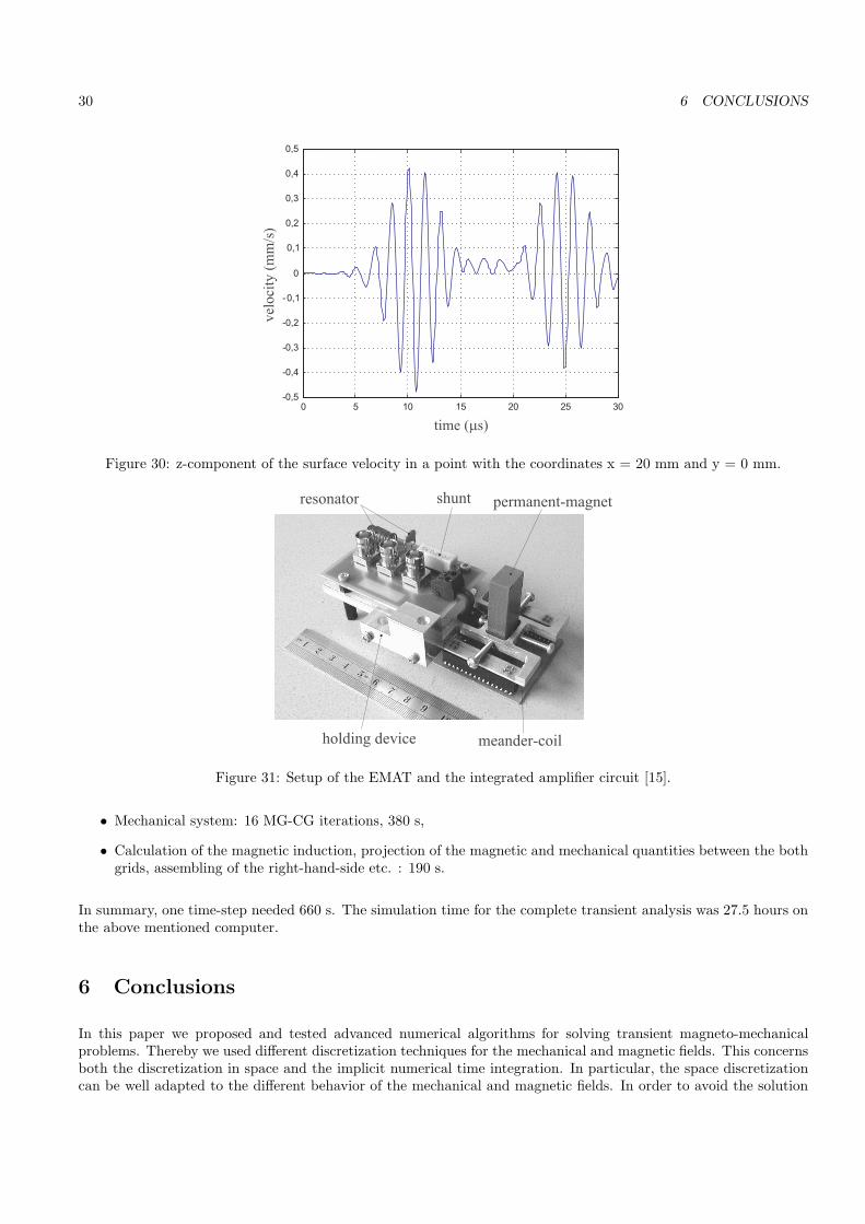
To measure the radiation pattern of the EMAT, the experimental setup which is shown in Fig. 31 is used. Toexcite the EMAT with sine burst of a frequency of 650 kHz, a RITEC System is used [32]. This system allows thegeneration of pulses with very high currents. In Fig. 32, the whole measurement setup is displayed. By use of the

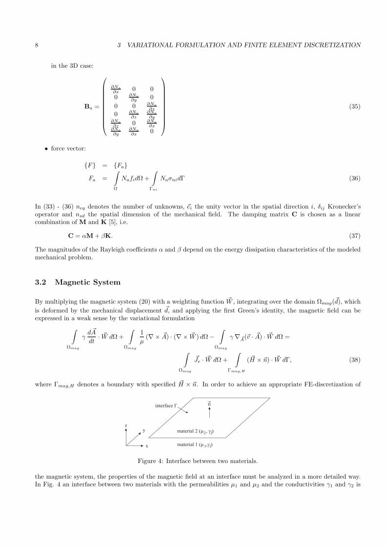
5.2 Electro-Magnetic-Acoustic-Transducer (EMAT) 29

x (mm)

x (mm)

y (

mm

)

y (

mm

)y

(m

m)

y (

mm

)

t = 10.0 sm

t = 13.0 sm

x (mm)

x (mm)

t = 11.5 sm

t = 15.0 sm

Figure 29: Transversal component of the Lamb wave at the surface of the aluminum plate.

RITEC system a current pulse in the meander coil is generated. The produced mechanical wave is detected withthe help of a laser-doppler vibrometer. The output signal of the vibrometer is filtered by the RITEC system andis then displayed on an oscilloscope. By measuring the maximum amplitude of the wave for different angles ϕ andconstant distance r of the vibrometer measurement point, the radiation characteristic can be obtained (see Fig. 33).To avoid to big errors of the measurement, the distance r must be out of the nearfield of the EMAT. The size of thenearfield can be estimated by the Fresnel distance [27]

rf = w2 k

10 π= 26.6 mm, (105)

where w denotes the length of the meander coil in y-direction and k = 2 π/λ the wave number. In the simulation,the amplitude of the radiated wave for different angles ϕ and the distance r was also used to determine the radiationpattern (see Fig. 33).

In Fig. 34, the measured and simulated radiation patterns are displayed. It can be seen that the main radiationdirection of the EMAT is in an angle of zero grad (y-direction), but there is also a radiation in other directions.These components can only be calculated by a full 3D simulation of the problem. The reason for the slight distortionof the symmetry of the radiation pattern with respect to the x-axis is the asymmetry of the meander coil.

5.2.6 Computation Times

The dynamical simulation of the Lamb wave in the plate needs an observation time of 15 µs. 150 time-steps arenecessary, because the time-step width of the simulation was chosen to be 100 ns. At each time step, the linear FEequation systems for the magnetic (342.000 degrees of freedom) and the mechanical (783.000 degrees of freedom)problems must be solved. This results in the following calculation times (SGI ORIGIN 300 MHz):

• Magnetic system: 6 MG-CG iterations, 90 s,

30 6 CONCLUSIONS

0 5 10 15 20 25 30-0,5

-0,4

-0,3

-0,2

-0,1

0

0,1

0,2

0,3

0,4

0,5

time ( s)m

vel

oci

ty (

mm

/s)

Figure 30: z-component of the surface velocity in a point with the coordinates x = 20 mm and y = 0 mm.

shunt

holding device meander-coil

resonator permanent-magnet

Figure 31: Setup of the EMAT and the integrated amplifier circuit [15].

• Mechanical system: 16 MG-CG iterations, 380 s,

• Calculation of the magnetic induction, projection of the magnetic and mechanical quantities between the bothgrids, assembling of the right-hand-side etc. : 190 s.

In summary, one time-step needed 660 s. The simulation time for the complete transient analysis was 27.5 hours onthe above mentioned computer.

6 Conclusions

In this paper we proposed and tested advanced numerical algorithms for solving transient magneto-mechanicalproblems. Thereby we used different discretization techniques for the mechanical and magnetic fields. This concernsboth the discretization in space and the implicit numerical time integration. In particular, the space discretizationcan be well adapted to the different behavior of the mechanical and magnetic fields. In order to avoid the solution

31

Transmitter

Laser-Doppler-Vibrometer

Control

Data

Trigger HF-Signal

Personal Computer

Figure 32: Setup to measure the radiation pattern of a Lamb wave EMAT.

Figure 33: Measurement of the radiation pattern of the EMAT with the help of a laser-doppler vibrometer.

of large systems of coupled mechanical and magnetic finite element equations at each time integration step, we useda coupling iteration procedure that successively requires the solution of mechanical and magnetic systems of finiteelement equations. The solution of these systems of finite element equations is certainly the most expensive partof the whole numerical algorithms. Whereas no efficient (i.e. linear complexity) solvers are known for the coupledsystem of mechanical and magnetic finite element equations, such solvers are individually available for the mechanicalsystem as well as for the magnetic system, namely multigrid solvers.

In the second part of the paper we applied our discretization and solution procedure to real-life magneto-mechanicalproblems and compared the results of our computer simulation with measurements obtained from the real counterpartof our virtual computer model. On the basis of both examples the applicability of the presented simulation-techniqueto real-life magneto-mechanical problems was demonstrated. The measured and simulated results showed a goodagreement. Also the simulation times were comparatively moderate.

Finally, we can summarize that the numerical algorithm proposed in this paper yields a software tool that allowsus to simulate quite complex magneto-mechanical sensor and actuator systems in a reasonable time. Therefore, theengineer can use this simulation software very well in the design process. The parallelization of the algorithm, thatmainly means the parallelization of the multigrid solvers (see [10, 11, 8]), will considerably accelerate the simulation

32 REFERENCES

-80 -60 -40 -20 0 20 40 60 800

0.2

0.4

0.6

0.8

1

no

rmal

ized

z-d

isp

lace

men

t

angle (degrees)

measurement3D simulation

Figure 34: Simulated and measured radiation pattern of a plate-wave EMAT (excitation frequency 0.65 MHz).

on an appropriate parallel computer. Then the simulation can be coupled with an optimization procedure.

Acknowledgements

This work has been supported by the Austrian Science Foundation - ‘Fonds zur Forderung der wissenschaftlichen Forschung(FWF)’ under project F1306 of the SFB F013 ‘Numerical and Symbolic Scientific Computing’.

Addresses: Ulrich Langer, Institut fur Numerische Mathematik, Johannes Kepler Universitat Linz, Altenberger-strasse 69, 4040 Linz, AustriaReinhard Lerch, Lehrstuhl fur Sensorik, Universitat Erlangen-Nurnberg, Paul-Gordan-Strasse 3/5,91052 Erlangen, GermanyMichael Schinnerl, Spezialforschungsbereich Numerical and Symbolic Scientific Computing, Univer-sitat Linz, Altenbergerstrasse 69, 4040 Linz, AustriaJoachim Schoberl, Spezialforschungsbereich Numerical and Symbolic Scientific Computing, JohannesKepler Universitat Linz, Altenbergerstrasse 69, 4040 Linz, AustriaManfred Kaltenbacher, Lehrstuhl fur Sensorik, Universitat Erlangen-Nurnberg, Paul-Gordan-Strasse 3/5, 91052 Erlangen, Germany

References

[1] D.N. Arnold, R.S. Falk, and R. Winther. Multigrid in H(div) and H(curl). Numer. Math., 85:197–218, 2000.

[2] O. Axelsson. Iterative Solution Methods. Cambridge University Press, 2 edition, 1996.

[3] F. Bachinger, U. Langer, and J. Schoberl. Numerical analysis of nonlinear multiharmonic eddy current problems.Numerische Mathematik, 100:593–616, 2005.

[4] Ballanyi. Handbuch Weicheisenprufer WP-C. 2000.

[5] K.J. Bathe. Finite Element Procedures. Prentice-Hall, New Jersey, 1996.

[6] W. Beitz and K.-H. Kuttner. Dubbel, Taschenbuch fur den Maschinenbau. Springer, Berlin, 17 edition, 1990.

[7] M. Costabel and M. Dauge. Weighted regularization of Maxwell equations in polyhedral domains. Numer.Math., 93(2):239–278, 2002.

REFERENCES 33

[8] C. Douglas, G. Haase, and U. Langer. A Tutorial on Elliptic PDE Solvers and Their Parallelization. SIAM,Philadelphia, 2003.

[9] K. Ettinger. Numerical Simulation of Electromagnetic Acoustic Transducers (EMATs). Diplomarbeit, Univer-sitat Linz, 1998.

[10] G. Haase, M. Kuhn, and U. Langer. Parallel multigrid 3d Maxwell solvers. Parallel Computing, 27(6):761–775,2001.

[11] G. Haase and U. Langer. Multigrid methods: From geometrical to algebraic versions. In A. Bourlioux andM.J. Gander, editors, Modern Methods in Scientific Computing and Applications, volume 75 of NATO ScienceSer. II, Mathematics, Physics and Chemistry, pages 103–153. Kluwer Academic Press, Dordrecht, 2002.

[12] W. Hackbusch. Multi-Grid Methods and Applications. Springer, Berlin, 1985.

[13] Hewlett-Packard. Handbuch Impedance/Gain Phase Analyzer 4194 A.

[14] R. Hiptmair. Multigrid methods for Maxwell’s equations. SIAM J. Numer. Anal., 36:204–225, 1999.

[15] M. Hofer. Simulation und Messung der Abstrahleigenschaften von Elektromagnetisch - Akustischen Transduc-ern. Diplomarbeit, Universitat Linz, 1999.

[16] T.J.R. Hughes. The Finite Element Method. Prentice-Hall, New Jersey, 1987.

[17] M. Jung and U. Langer. Applications of multilevel methods to practical problems. Surv. Math. Ind., 1:217–257,1991.

[18] E. Kallenbach, R. Eick, and P. Quendt. Elektromagnete. Teubner, Stuttgart, 1994.

[19] M. Kaltenbacher. Numerical Simulation of Mechatronic Sensors and Actuators. Springer, Berlin, Heidelberg,New York, 2004.

[20] M. Kaltenbacher, H. Landes, and R. Lerch. An Efficient Calculation Scheme for the Numerical Simulation ofCoupled Magnetomechanical Systems. IEEE Transactions on Magnetics, 33(2):1646–1649, 1997.

[21] M. Kaltenbacher, H. Landes, and R. Lerch. CAPA Verification Manual, Release 3. 1999.

[22] G.S. Kino. Acoustic Waves - Devices, Imaging & Analog Signal Processing. Prentice Hall Inc., 1987.

[23] J. Krautkramer and H. Krautkramer. Werkstoffprufung mit Ultraschall. Springer, Berlin, 5 edition, 1986.

[24] S. Kurz, J. Fetzer, G. Lehner, and W. Rucker. A novel formulation for 3d eddy current problems with movingbodies using a lagrangian description and bem-fem coupling. IEEE Transactions on Magnetics, 34(5):3068–3073,1998.

[25] R. Lerch. Elektrische Messtechnik. Springer, 2004.

[26] R. Ludwig and X.-W. Dai. Numerical simulation of electromagnetic acoustic transducer in the time domain.J.Appl.Phys., 69(1):89–98, 1991.

[27] D.P. Morgan. SAW Devices and Signal Processing. Elsevier, Amsterdam, 1991.

[28] J. Nedelec. Mixed finite elements in R3. Numer.Math., pages 315–341, 1980.

[29] Polytec. Handbuch Polytec Laser Doppler Vibrometer. 1999.

[30] S. Reitzinger and J. Schoberl. An algebraic multigrid method for finite element discretizations with edgeelements. Numer. Linear Algebra Appl., 31(3):223–238, 2002.

[31] Z. Ren and A. Razek. A Strong Coupled Model for Analysing Dynamic Behaviours of Non-linear ElectromagneticSystems. IEEE Transactions on Magnetics, 30(5):3252–3255, 1994.

[32] RITEC. Operation Manual for Advanced Measurement System Model RAM-0.25-17.5. 1997.

34 REFERENCES

[33] M. Schinnerl. Numerische Berechnung magneto-mechanischer Systeme mit Mehrgitterverfahren. Dissertation,Universitat Erlangen-Nurnberg, 2001.

[34] K.P. Schmitz. Entwicklung und Untersuchung einer schnellschaltenden elektromagnetischen Stelleinheit. Dis-sertation, TU Aachen, 1988.

[35] P.S. Silvester and R.L. Ferrari. Finite elements for electrical engineers. Cambridge University Press, 3 edition,1996.

[36] J. A. Stratton. Electromagnetic Theory. McGraw-Hill, Inc., 1941.

[37] G. Wunsch and H. Schulz. Elektromagnetische Felder. Verlag Technik, Berlin, 2 edition, 1996.

[38] F. Ziegler. Mechanics of Solids and Fluids. Springer, Vienna, 1991.