1 Observability and controllability analysis of linear systems … · · 2016-09-201 Observability and controllability analysis of linear systems subject to data losses Raphael

1

Observability and controllability analysis of

linear systems subject to data losses

Raphael M. Jungers, Atreyee Kundu, W.P.M.H. (Maurice) Heemels

Abstract

We provide algorithmically verifiable necessary and sufficient conditions for fundamental system

theoretic properties of discrete-time linear systems subject to data losses. More precisely, the systems

in our modeling framework are subject to disruptions (data losses) in the feedback loop, where the

set of possible data loss sequences is captured by an automaton. As such, the results are applicable in

the context of shared (wireless) communication networks and/or embedded architectures where some

information on the data loss behaviour is available a priori.

We propose an algorithm for deciding observability (or the absence of it) for such systems, and show

how this algorithm can be used also to decide other properties including constructibility, controllability,

reachability, null-controllability, detectability and stabilizability by means of relations that we establish

among these properties. The main apparatus for our analysis is the celebrated Skolem’s Theorem from

linear algebra.

Moreover, we study the relation between the model adopted in this paper and a previously introduced

model where, instead of allowing dropouts in the feedback loop, one allows for time-varying delays.

Index Terms

R. M. Jungers is with the Cyber-Physical Systems Laboratory at the University of California, Los Angeles (on sabbatical

leave from UCLouvain, Belgium). A. Kundu and W.P.M.H. Heemels are with the Control Systems Technology Group,

Department of Mechanical Engineering, Eindhoven University of Technology, 5600 MB Eindhoven, The Netherlands. Emails:

[email protected], [email protected], [email protected].

Raphael is supported by the Communaute francaise de Belgique, by the Belgian Programme on Interuniversity Attraction

Poles, and the Fulbright Commission. He is a F.R.S.-FNRS Research Associate.

Maurice is supported by the Innovational Research Incentives Scheme under the VICI grant “Wireless control systems: A

new frontier in automation” (no. 11382) awarded by NWO (Netherlands Organisation for Scientific Research), and STW (Dutch

Science Foundation), and the STW project 12697 “Control based on data-intensive sensing.”

September 20, 2016 DRAFT

arX

iv:1

609.

0584

0v1

[m

ath.

OC

] 1

9 Se

p 20

16

2

Data losses, Wireless Control, Constrained Switched System, Automaton, Observability, Controlla-

bility

I. Introduction

The last decades have witnessed the introduction of many sensing, computing and wireless communi-

cation devices in a broad range of control applications leading to networked control and cyber-physical

systems. In such systems it is observed that the phenomenon of data losses is rather common as a real-

time feedback loop can be disrupted intermittently by packet losses in wireless communication, task

deadlines can be missed in shared embedded processors, outliers can be discarded in sensor-harvested

data, and so on. This has caused a vivid interest in the analysis and design of control systems, see, e.g.,

[3], [8], [10], [20], [22], [23], [25], [28] and the references therein.

As data losses lead to imperfect control updates, it can be expected that fundamental system theo-

retic properties such as observability, controllability, detectability, stabilizability, etc. are affected. These

fundamental notions have played central roles throughout the history of modern control theory and have

been studied extensively in the context of finite-dimensional linear systems, nonlinear systems, infinite-

dimensional systems, n-dimensional systems, hybrid systems, and behavioral systems. One may refer, for

instance, to [26] for historical comments and references. Given the importance of these notions on the one

hand and the relevance of cyber-physical and networked control systems on the other hand, we believe

that observability (and related notions) under packet loss will be critical in forthcoming engineering

applications.

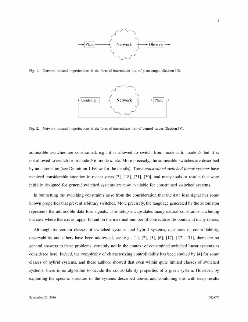
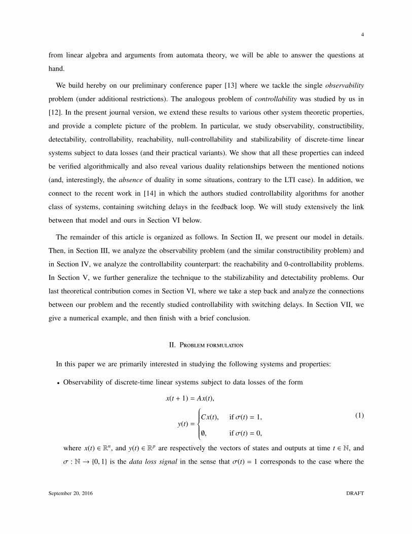
Figures 1 and 2 illustrate two situations of intermittent data losses that are of interest and will be studied

in the present paper. It is rather remarkable that these questions have not been answered despite the large

literature on systems with packet loss. The above-mentioned references have introduced (analysis and

design) methods that can guarantee stability of the closed-loop systems (up to some conservativeness), but

to our knowledge the fundamental properties in dropout systems have not been studied from a theoretical

and algorithmic point of view, as they have been for linear (and, later, for nonlinear) systems.

Motivated by these considerations, we will address in this paper the problem of studying observability,

controllability, detectability, stabilizability and other fundamental properties for discrete-time linear time-

invariant (LTI) systems with packet losses represented in Figures 1 and 2. We will also study the

relationships between these notions. We employ a constrained switched systems perspective for modelling

the system under consideration. A constrained switched system is a switched system in which the


3

Plant ObserverNetwork

Fig. 1. Network-induced imperfections in the form of intermittent loss of plant output (Section III).

Controller PlantNetwork

Fig. 2. Network-induced imperfections in the form of intermittent loss of control values (Section IV).

admissible switches are constrained, e.g., it is allowed to switch from mode a to mode b, but it is

not allowed to switch from mode b to mode a, etc. More precisely, the admissible switches are described

by an automaton (see Definition 1 below for the details). These constrained switched linear systems have

received considerable attention in recent years [7], [18], [21], [30], and many tools or results that were

initially designed for general switched systems are now available for constrained switched systems.

In our setting the switching constraints arise from the consideration that the data loss signal has some

known properties that prevent arbitrary switches. More precisely, the language generated by the automaton

represents the admissible data loss signals. This setup encapsulates many natural constraints, including

the case where there is an upper bound on the maximal number of consecutive dropouts and many others.

Although for certain classes of switched systems and hybrid systems, questions of controllability,

observability and others have been addressed, see, e.g., [1], [2], [5], [6], [17], [27], [31], there are no

general answers to these problems, certainly not in the context of constrained switched linear systems as

considered here. Indeed, the complexity of characterizing controllability has been studied by [4] for some

classes of hybrid systems, and these authors showed that even within quite limited classes of switched

systems, there is no algorithm to decide the controllability properties of a given system. However, by

exploiting the specific structure of the systems described above, and combining this with deep results


4

from linear algebra and arguments from automata theory, we will be able to answer the questions at

hand.

We build hereby on our preliminary conference paper [13] where we tackle the single observability

problem (under additional restrictions). The analogous problem of controllability was studied by us in

[12]. In the present journal version, we extend these results to various other system theoretic properties,

and provide a complete picture of the problem. In particular, we study observability, constructibility,

detectability, controllability, reachability, null-controllability and stabilizability of discrete-time linear

systems subject to data losses (and their practical variants). We show that all these properties can indeed

be verified algorithmically and also reveal various duality relationships between the mentioned notions

(and, interestingly, the absence of duality in some situations, contrary to the LTI case). In addition, we

connect to the recent work in [14] in which the authors studied controllability algorithms for another

class of systems, containing switching delays in the feedback loop. We will study extensively the link

between that model and ours in Section VI below.

The remainder of this article is organized as follows. In Section II, we present our model in details.

Then, in Section III, we analyze the observability problem (and the similar constructibility problem) and

in Section IV, we analyze the controllability counterpart: the reachability and 0-controllability problems.

In Section V, we further generalize the technique to the stabilizability and detectability problems. Our

last theoretical contribution comes in Section VI, where we take a step back and analyze the connections

between our problem and the recently studied controllability with switching delays. In Section VII, we

give a numerical example, and then finish with a brief conclusion.

II. Problem formulation

In this paper we are primarily interested in studying the following systems and properties:

• Observability of discrete-time linear systems subject to data losses of the form

x(t + 1) = Ax(t),

y(t) =

Cx(t), if σ(t) = 1,

∅, if σ(t) = 0,

(1)

where x(t) ∈ Rn, and y(t) ∈ Rp are respectively the vectors of states and outputs at time t ∈ N, and

σ : N → {0, 1} is the data loss signal in the sense that σ(t) = 1 corresponds to the case where the


5

output is available at time t ∈ N, and σ(t) = 0 corresponds to the case where the output is lost at

time t ∈ N.

• Controllability of discrete-time linear systems subject to data losses of the form

x(t + 1) =

Ax(t) + Bu(t), if σ(t) = 1,

Ax(t), if σ(t) = 0,(2)

where x(t) ∈ Rn, and u(t) ∈ Rm are respectively the vectors of states and inputs at time t ∈ N, and

σ : N → {0, 1} is the data loss signal in the sense that σ(t) = 1 corresponds to the case where the

input is effectively conveyed to the plant at time t ∈ N, and σ(t) = 0 corresponds to the case where

the input is lost at time t ∈ N.

For any pair of matrices (A,C) (resp. (A, B)), the observability (resp. controllability) problem is relevant

only if some additional assumptions are made on the possible dropout behaviour (it is obvious that if

σ(t) = 0 for all t ∈ N, the system is not observable (resp. not controllable)). For this reason, our model

comes with certain constraints on the classes of data loss signals σ. For example, a natural assumption

is that there can be at most ` ∈ N consecutive data losses with ` given. Such constraints on the data

loss signal are often encountered in practice, and arise from the characteristics of the shared (wireless)

communication network and/or the embedded architecture. Another type of constraints could be that

for every m consecutive time steps, we receive data in good order on at least k time steps (so-called

(m, k)-firmness), where m, k ∈ N are given parameters [9], [11], [29].

All the above constraints (and many others) on the data loss signal can be captured by an automaton,

which is part of the description of the dynamical system. We now formally describe this notion (which

slightly deviates from the literature to satisfy our needs).

Definition 1: An automaton is a pair A = (M, s) ∈ {0, 1}N×N ×{0, 1}N , where N is the number of nodes

(or states), M ∈ {0, 1}N×N is the transition matrix, and s = (s1 s2 . . . sN)> ∈ {0, 1}N is the vector of node

labels.

Definition 2: A data loss signal σ : N→ {0, 1} is said to be admissible with respect to an automaton

A = (M, s) with N nodes, if there exists a sequence of states v : N→ {1, 2, . . . ,N} such that for all t ∈ N

it holds that Mv(t),v(t+1) = 1 and σ(t) = sv(t). The set of all admissible data loss signals for the automaton

A is denoted by L(A).

In this paper we consider only automata that can produce at least one admissible data loss signal (and

thus by definition defined for all t ∈ N), which implies that the automaton must contain at least one cycle.


6

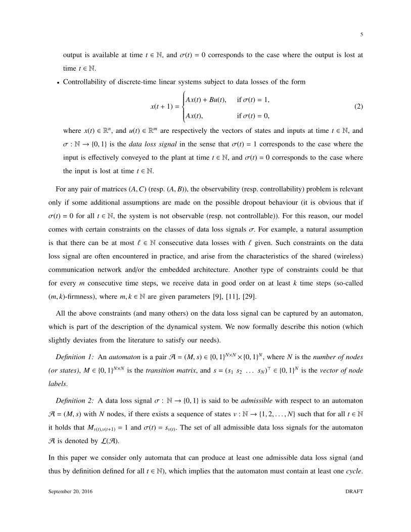
Example 1: Consider a control system where there can be at most ` ∈ N consecutive data losses. This

can be captured by an automaton containing ` + 1 nodes, in which the node i ∈ {1, 2, · · · , `} represents

the situation where the data generated at the last i consecutive instants were lost, and the one before

arrived safely. The node `+ 1 represents the situation where the last packet arrived safely. Let ` = 3. The

corresponding automaton A = (M, s) with M =

0 1 0 1

0 0 1 1

0 0 0 1

1 0 0 1

and s =

0

0

0

1

is shown in Figure 3.

s4 = 1 s3 = 0

s1 = 0 s2 = 0

Fig. 3. Automaton representing data loss signals with at most 3 consecutive losses. Labels are represented directly on the

nodes.

Combining the description of the dynamics (1) (or (2)) and the automaton A, our systems can be modeled

as so-called discrete-time constrained switched linear systems. These systems, where the switching signal

is constrained by an automaton, have been the subject of much attention recently [7], [18], [21], [30],

see also the introduction.

In the sequel we refer to the discrete-time switched systems (1) and (2) constrained by an automaton

A with the tuples (A,C,A) and (A, B,A), respectively. Similarly, the notations x(t, x0, σ) and y(t, x0, σ)

denote the state and output trajectories of the system (1) at time t ∈ N generated under a switching signal

σ with initial state x0. The notation x(t, x0, u, σ) denotes the state and output trajectories of the system

(2) at time t ∈ N generated under a switching signal σ and control input signal u : N→ Rm with initial

state x0. However, when there is no ambiguity, we stick to x(t) and y(t) for brevity.

Definition 3: (i) The system (A,C,A) is said to be observable if for any σ ∈ L(A), any pair of initial

states x0 and x0 ∈ Rn, it holds that y(t, x0, σ) = y(t, x0, σ) for all t ∈ N implies that x0 = x0. The system

is called unobservable otherwise.


7

(ii) The system (A,C,A) is said to be constructible if for any σ ∈ L(A), and any initial state x0,

there exists a T ∈ N such that for any x0 ∈ Rn that satisfies y(t, x0, σ) = y(t, x0, σ) for all t ∈ N[0,T ] it

holds that x(T, x0, σ) = x(T, x0, σ). The system is called non-constructible otherwise.

(iii) The system (A,C,A) is said to be detectable if for any σ ∈ L(A) and any initial state x0 ∈ Rn with

y(t, x0, σ) = 0 for all t ∈ N, it holds that x(t, x0, σ) → 0 as t → ∞. The system is called undetectable

otherwise.

Definition 4: (i) The system (A, B,A) is said to be controllable if for any σ ∈ L(A), any initial state

x0 ∈ Rn and any final state x f ∈ R

n, there is an input signal u : N→ Rm such that x(T, x0, u, σ) = x f for

some T ∈ N. The system is called uncontrollable otherwise.

(ii) The system (A, B,A) is said to be reachable if for any σ ∈ L(A), and for the initial state 0 ∈ Rn

and any final state x f ∈ Rn, there is an input signal u : N → Rm such that x(T, x0, u, σ) = x f for some

T ∈ N. The system is called unreachable otherwise.

(iii) The system (A, B,A) is said to be 0-controllable if for any σ ∈ L(A) and any initial state x0 ∈ Rn,

there is an input signal u : N → Rm such that x(T, x0, u, σ) = 0 for some T ∈ N. The system is called

non-0-controllable otherwise.

(iv) The system (A, B,A) is said to be stabilizable if for any σ ∈ L(A) and any initial state x0 ∈ Rn, there

is an input signal u : N → Rm such that limt→∞ x(t, x0, u, σ) = 0. The system is called non-stabilizable

otherwise.

To motivate the study of these properties, let us consider an example.

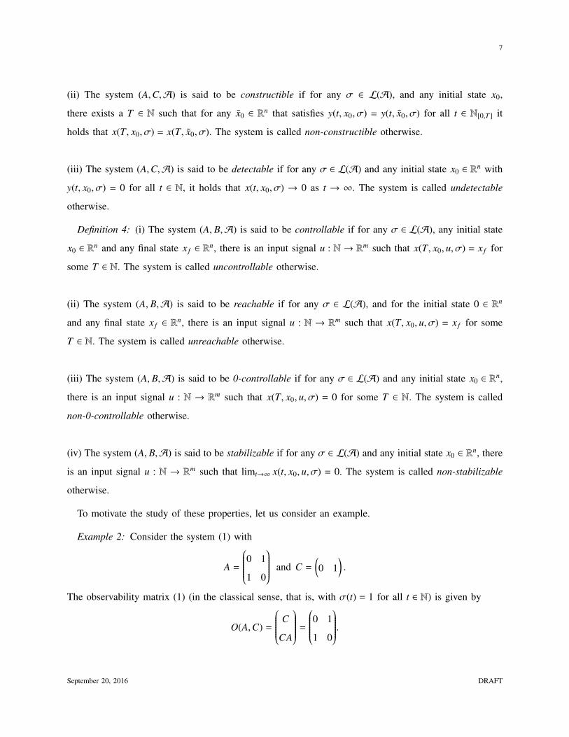
Example 2: Consider the system (1) with

A =

0 1

1 0

and C =

(0 1

).

The observability matrix (1) (in the classical sense, that is, with σ(t) = 1 for all t ∈ N) is given by

O(A,C) =

C

CA

=

0 1

1 0

.


8

Notice that the rank of O(A,C) is 2, and consequently, the pair (A,C) is observable in the classical sense.

Let us now suppose that the system is subject to dropout signals, as described by the automaton A in

Figure 3. Under the periodic data loss signal σ = (1, 0, 1, 0, 1, 0, . . .), which is admissible with respect to

A, it is easy to see that the system is no longer observable.

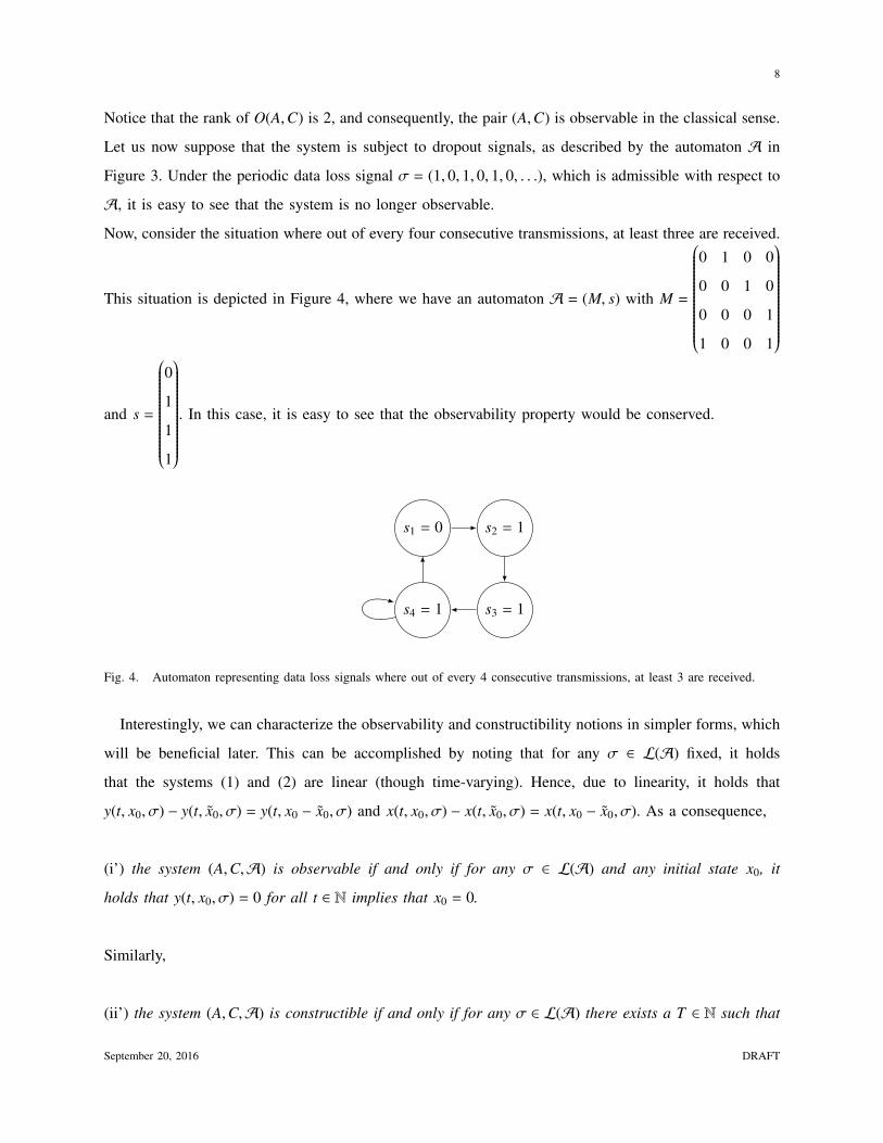
Now, consider the situation where out of every four consecutive transmissions, at least three are received.

This situation is depicted in Figure 4, where we have an automaton A = (M, s) with M =

0 1 0 0

0 0 1 0

0 0 0 1

1 0 0 1

and s =

0

1

1

1

. In this case, it is easy to see that the observability property would be conserved.

s4 = 1 s3 = 1

s1 = 0 s2 = 1

Fig. 4. Automaton representing data loss signals where out of every 4 consecutive transmissions, at least 3 are received.

Interestingly, we can characterize the observability and constructibility notions in simpler forms, which

will be beneficial later. This can be accomplished by noting that for any σ ∈ L(A) fixed, it holds

that the systems (1) and (2) are linear (though time-varying). Hence, due to linearity, it holds that

y(t, x0, σ) − y(t, x0, σ) = y(t, x0 − x0, σ) and x(t, x0, σ) − x(t, x0, σ) = x(t, x0 − x0, σ). As a consequence,

(i’) the system (A,C,A) is observable if and only if for any σ ∈ L(A) and any initial state x0, it

holds that y(t, x0, σ) = 0 for all t ∈ N implies that x0 = 0.

Similarly,

(ii’) the system (A,C,A) is constructible if and only if for any σ ∈ L(A) there exists a T ∈ N such that


9

for any x0 ∈ Rn that satisfies y(t, x0, σ) = 0 for all t ∈ N[0,T ] it holds that x(T, x0, σ) = 0.

Remark 1: We now introduce a variant of our notions, which might be of practical importance, where

the critical time T in the definitions does not depend on the particular packet loss signal, nor the initial

state.

The system (A,C,A) is said to be practically observable if there exists a T ∈ N such that for any

σ ∈ L(A), any pair of initial states x0 and x0 ∈ Rn with y(t, x0, σ) = y(t, x0, σ) for all t ∈ N[0,T ], it

holds that x0 = x0. Similarly, (A,C,A) is said to be practically constructible if there exists a T ∈ N

such that for all σ ∈ L(A), and all initial states x0 and x0 ∈ Rn with y(t, x0, σ) = y(t, x0, σ) for all

t ∈ N[0,T ] it holds that x(T, x0, σ) = x(T, x0, σ). Hence, in the ‘practical’ version of the observability and

constructibility notions, the time T can be taken independently of x0 and σ, which is obviously more

practical for reconstructing initial states from the output data and the data loss signal. In fact, we will show

below that the observability (resp. constructibility) property formulated in Definition 3-(i) (resp. (ii)) is

equivalent to practical observability (resp. practical constructibility) as defined here. Similar observations

apply to the controllability, reachability and 0-controllability notions for which practical versions can be

defined as follows. The system (A, B,A) is said to be practically controllable if there exists a time T ∈ N

such that for any σ ∈ L(A), any initial state x0 ∈ Rn and any final state x f ∈ R

n, there is an input signal

u : N → Rm such that x(t, x0, u, σ) = x f for some t ∈ N≤T . It is said to be practically reachable if there

exists a T ∈ N such that for any σ ∈ L(A), and for the initial state 0 ∈ Rn and any final state x f ∈ Rn,

there is an input signal u : N → Rm such that x(t, x0, u, σ) = x f for some t ∈ N≤T . Finally, the system

(A, B,A) is said to be practically 0-controllable if there exists T ∈ N such that for any σ ∈ L(A) and

any initial state x0 ∈ Rn, there is an input signal u : N→ Rm such that x(t, x0, u, σ) = 0 for some t ∈ N≤T .

Note that all the given properties are invariant under similarity transformations. As such, we have, for

instance, (A,C,A) is observable if and only (S AS −1,CS −1,A) is observable, and (A, B,A) is controllable

if and only if (S AS −1, S B,A) is controllable, in which S ∈ Rn×n is an invertible matrix.

III. Observability results

In this section we tackle the following problem:

Problem 1: Given a constrained discrete-time switched linear system (1) specified by the triple (A,C,A),

determine whether the system is (un)observable and (non-)constructible.


10

We provide algorithmically verifiable necessary and sufficient conditions to the above problem thereby

proving its decidability. In fact, the observability property can be formalized in a completely algebraic

way, in terms of an observability matrix, just like in the classical case.

Definition 5: Given a data loss signal σ : N→ {0, 1}, we define the observability matrix of the system

(A,C,A) for σ at time t ∈ N by

Oσ(t) :=

σ(0)C

σ(1)CA...

σ(t − 1)CAt−1

∈ Rtp×n. (3)

Proposition 1: The system (A,C,A) is observable if and only if for all σ ∈ L(A) there exists a t ∈ N

such that the observability matrix Oσ(t) is of rank n.

Proof: (Necessity) We employ contradiction. Suppose that the system (A,C,A) is observable, but

there exists a σ ∈ L(A) and a nonzero α ∈ Rn such that for all t, Oσ(t)α = 0 (note that the null space

of Oσ(t) is a superset of the null space of Oσ(t + 1) for all t ∈ N). Pick x(0) = x0 = α. Then y(t) = 0 for

all t ∈ N. Hence, based on (i’), the system (A,C,A) is unobservable.

(Sufficiency) Given that for all admissible σ, there is a t ∈ N such that Oσ(t) has full rank, x(0) can be

uniquely obtained from

y(0)...

y(t)

= Oσ(t)x0. The observability of the system (A,C,A) follows.

Based on this proposition we sometimes call a σ : N → {0, 1} observable if the corresponding

observability matrix has full rank for some t ∈ N. Otherwise, we say that the data loss signal σ is

unobservable.

Note that this proposition shows that

(i”) the system (A,C,A) is observable if and only if for any σ ∈ L(A) there is a T ∈ N such that

for any initial state x0 with y(t, x0, σ) = 0 for t ∈ N[0,T ] it holds that x0 = 0.

Note that the difference with respect to practical observability lies in the fact that for practical observability

T is independent of σ ∈ L(A).

It is well known that for LTI systems, the difference between observability and constructibility lies in

the (un)observability of the modes associated with zero eigenvalues. We now generalize this result to our


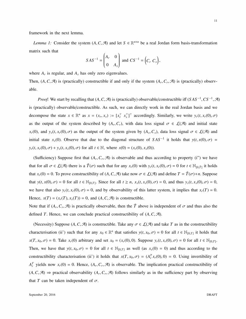
11

framework in the next lemma.

Lemma 1: Consider the system (A,C,A) and let S ∈ Rn×n be a real Jordan form basis-transformation

matrix such that

S AS −1 =

Ar 0

0 As

and CS −1 =

(Cr Cs

),

where Ar is regular, and As has only zero eigenvalues.

Then, (A,C,A) is (practically) constructible if and only if the system (Ar,Cr,A) is (practically) observ-

able.

Proof: We start by recalling that (A,C,A) is (practically) observable/constructible iff (S AS −1,CS −1,A)

is (practically) observable/constructible. As such, we can directly work in the real Jordan basis and we

decompose the state x ∈ Rn as x = (xr, xs) := [x>r x>s ]> accordingly. Similarly, we write yr(t, xr(0), σ)

as the output of the system described by (Ar,Cr), with data loss signal σ ∈ L(A) and initial state

xr(0), and ys(t, xr(0), σ) as the output of the system given by (As,Cs), data loss signal σ ∈ L(A) and

initial state xs(0). Observe that due to the diagonal structure of S AS −1 it holds that y(t, x(0), σ) =

yr(t, xr(0), σ) + ys(t, xs(0), σ) for all t ∈ N, where x(0) = (xr(0), xs(0)).

(Sufficiency) Suppose first that (Ar,Cr,A) is observable and thus according to property (i”) we have

that for all σ ∈ L(A) there is a T (σ) such that for any xr(0) with yr(t, xr(0), σ) = 0 for t ∈ N[0,T ] it holds

that xr(0) = 0. To prove constructibility of (A,C,A) take now σ ∈ L(A) and define T = T (σ)+n. Suppose

that y(t, x(0), σ) = 0 for all t ∈ N[0,T ]. Since for all t ≥ n, xs(t, xs(0), σ) = 0, and thus ys(t, xs(0), σ) = 0,

we have that also yr(t, xr(0), σ) = 0, and by observability of this latter system, it implies that xr(T ) = 0.

Hence, x(T ) = (xr(T ), xs(T )) = 0, and (A,C,A) is constructible.

Note that if (Ar,Cr,A) is practically observable, then the T above is independent of σ and thus also the

defined T . Hence, we can conclude practical constructibility of (A,C,A).

(Necessity) Suppose (A,C,A) is constructible. Take any σ ∈ L(A) and take T as in the constructibility

characterisation (ii’) such that for any x0 ∈ Rn that satisfies y(t, x0, σ) = 0 for all t ∈ N[0,T ] it holds that

x(T, x0, σ) = 0. Take xr(0) arbitrary and set x0 = (xr(0), 0). Suppose yr(t, xr(0), σ) = 0 for all t ∈ N[0,T ].

Then, we have that y(t, x0, σ) = 0 for all t ∈ N[0,T ] as well (as xs(0) = 0) and thus according to the

constructibility characterisation (ii’) it holds that x(T, x0, σ) = (ATr xr(0), 0) = 0. Using invertibility of

ATr yields now xr(0) = 0. Hence, (Ar,Cr,A) is observable. The implication practical constructibility of

(A,C,A) ⇒ practical observability (Ar,Cr,A) follows similarly as in the sufficiency part by observing

that T can be taken independent of σ.


12

Corollary 1: If the system (A,C,A) is observable, then it is constructible. Moreover, if A is invertible,

then constructibility and observability are equivalent.

Proof: For the first part of the corollary, it follows directly from the observability characterisation

(i”) and the constructibility characterisation (ii’) (as x(T, x0, σ) = AT x0). The second part of the corollary

is obvious from Lemma 1.

We now turn to the main result of this section, which will allow us to decide observability. As announced

above, we will make use of the Skolem’s Theorem [19], [24] of Linear Algebra, which is given next.

Theorem 1: Consider a matrix A ∈ Rn×n and two vectors b, c ∈ Rn. The set of values of t ∈ N such

that c>Atb = 0 is eventually periodic in the sense that there exist two numbers P,T ∈ N such that

∀t ∈ N>T , c>Atb = 0 ⇔ c>At+Pb = 0. (4)

Moreover, the period P can be computed explicitly. In particular, if the entries in A, b, c are rational

numbers, P can be chosen smaller or equal to rn2, where r is any prime number not dividing det(mA),

and m is the least common multiple of the denominators of the entries in A.

The above theorem shows that if one is interested in the patterns of times such that the response of a

linear system x(t + 1) = Ax(t) with x(0) = b is confined to a linear subspace ker c> := {w ∈ Rn | c>w = 0},

then one can restrict the attention eventually to periodic patterns.

We now present our main result. In the course of its proof, we will need the following elementary

result, which connects observability and the practical versions (see Remark 1).

Lemma 2: The system (A,C,A) is practically observable (resp. practically constructible) if and only

if it is observable (resp. constructible).

Proof: The ‘only if’-part is obvious. For the ‘if’-part, let us suppose that the system is observable.

We have to show that there exists a T ∗ ∈ N such that for any σ ∈ L(A) and any initial state x0 ∈ Rn

with y(t, x0, σ) = 0 for all t ∈ N[0,T ∗] it holds that x0 = 0. Suppose by contradiction that for every T ∗ ∈ N

there is a σT ∗ with y(t, x0, σT ∗) = 0 for all t ∈ N[0,T ∗], but x0 , 0. Since

y(0)...

y(T ∗)

= OσT∗ (T ∗)x0 = 0,


13

we conclude that the observability matrix OσT∗ (T ∗) does not have full rank. This implies the existence of

an infinite signal σ such that Oσ(t) has never full rank, which leads to a contradiction. (The existence of

σ can be easily proved, e.g., by the convergence of the sequence {σT ∗}T ∗∈N w.r.t. the standard topology

on words, see the proof of Lemma 4 below for more details.)

The equivalence between constructibility and practical constructibility follows now from Lemma 1.

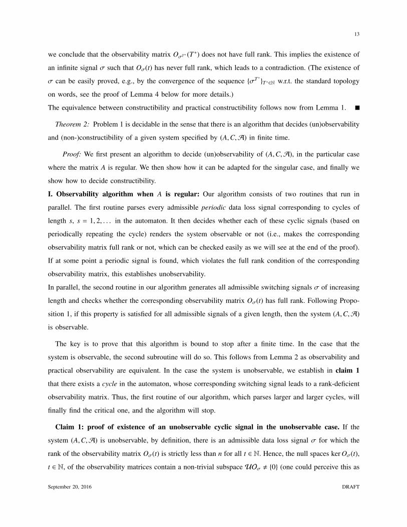
Theorem 2: Problem 1 is decidable in the sense that there is an algorithm that decides (un)observability

and (non-)constructibility of a given system specified by (A,C,A) in finite time.

Proof: We first present an algorithm to decide (un)observability of (A,C,A), in the particular case

where the matrix A is regular. We then show how it can be adapted for the singular case, and finally we

show how to decide constructibility.

I. Observability algorithm when A is regular: Our algorithm consists of two routines that run in

parallel. The first routine parses every admissible periodic data loss signal corresponding to cycles of

length s, s = 1, 2, . . . in the automaton. It then decides whether each of these cyclic signals (based on

periodically repeating the cycle) renders the system observable or not (i.e., makes the corresponding

observability matrix full rank or not, which can be checked easily as we will see at the end of the proof).

If at some point a periodic signal is found, which violates the full rank condition of the corresponding

observability matrix, this establishes unobservability.

In parallel, the second routine in our algorithm generates all admissible switching signals σ of increasing

length and checks whether the corresponding observability matrix Oσ(t) has full rank. Following Propo-

sition 1, if this property is satisfied for all admissible signals of a given length, then the system (A,C,A)

is observable.

The key is to prove that this algorithm is bound to stop after a finite time. In the case that the

system is observable, the second subroutine will do so. This follows from Lemma 2 as observability and

practical observability are equivalent. In the case the system is unobservable, we establish in claim 1

that there exists a cycle in the automaton, whose corresponding switching signal leads to a rank-deficient

observability matrix. Thus, the first routine of our algorithm, which parses larger and larger cycles, will

finally find the critical one, and the algorithm will stop.

Claim 1: proof of existence of an unobservable cyclic signal in the unobservable case. If the

system (A,C,A) is unobservable, by definition, there is an admissible data loss signal σ for which the

rank of the observability matrix Oσ(t) is strictly less than n for all t ∈ N. Hence, the null spaces ker Oσ(t),

t ∈ N, of the observability matrices contain a non-trivial subspace UOσ , {0} (one could perceive this as


14

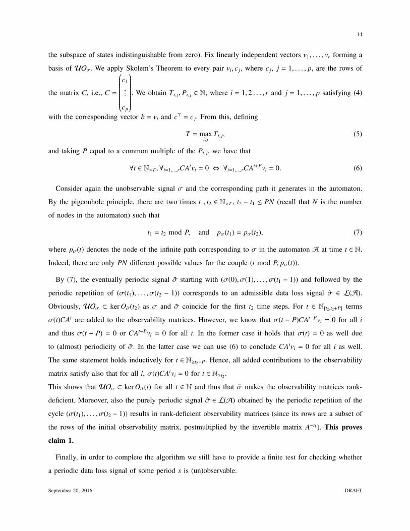
the subspace of states indistinguishable from zero). Fix linearly independent vectors v1, . . . , vr forming a

basis of UOσ. We apply Skolem’s Theorem to every pair vi, c j, where c j, j = 1, . . . , p, are the rows of

the matrix C, i.e., C =

c1...

cp

. We obtain Ti, j, Pi, j ∈ N, where i = 1, 2 . . . , r and j = 1, . . . , p satisfying (4)

with the corresponding vector b = vi and c> = c j. From this, defining

T = maxi, j

Ti, j, (5)

and taking P equal to a common multiple of the Pi, j, we have that

∀t ∈ N>T ,∀i=1,...,rCAtvi = 0 ⇔ ∀i=1,...,rCAt+Pvi = 0. (6)

Consider again the unobservable signal σ and the corresponding path it generates in the automaton.

By the pigeonhole principle, there are two times t1, t2 ∈ N>T , t2 − t1 ≤ PN (recall that N is the number

of nodes in the automaton) such that

t1 = t2 mod P, and pσ(t1) = pσ(t2), (7)

where pσ(t) denotes the node of the infinite path corresponding to σ in the automaton A at time t ∈ N.

Indeed, there are only PN different possible values for the couple (t mod P, pσ(t)).

By (7), the eventually periodic signal σ starting with (σ(0), σ(1), . . . , σ(t1 − 1)) and followed by the

periodic repetition of (σ(t1), . . . , σ(t2 − 1)) corresponds to an admissible data loss signal σ ∈ L(A).

Obviously, UOσ ⊂ ker Oσ(t2) as σ and σ coincide for the first t2 time steps. For t ∈ N[t2,t2+P] terms

σ(t)CAt are added to the observability matrices. However, we know that σ(t − P)CAt−Pvi = 0 for all i

and thus σ(t − P) = 0 or CAt−Pvi = 0 for all i. In the former case it holds that σ(t) = 0 as well due

to (almost) periodicity of σ. In the latter case we can use (6) to conclude CAtvi = 0 for all i as well.

The same statement holds inductively for t ∈ N≥t2+P. Hence, all added contributions to the observability

matrix satisfy also that for all i, σ(t)CAtvi = 0 for t ∈ N≥t2 .

This shows that UOσ ⊂ ker Oσ(t) for all t ∈ N and thus that σ makes the observability matrices rank-

deficient. Moreover, also the purely periodic signal σ ∈ L(A) obtained by the periodic repetition of the

cycle (σ(t1), . . . , σ(t2 − 1)) results in rank-deficient observability matrices (since its rows are a subset of

the rows of the initial observability matrix, postmultiplied by the invertible matrix A−t1). This proves

claim 1.

Finally, in order to complete the algorithm we still have to provide a finite test for checking whether

a periodic data loss signal of some period s is (un)observable.


15

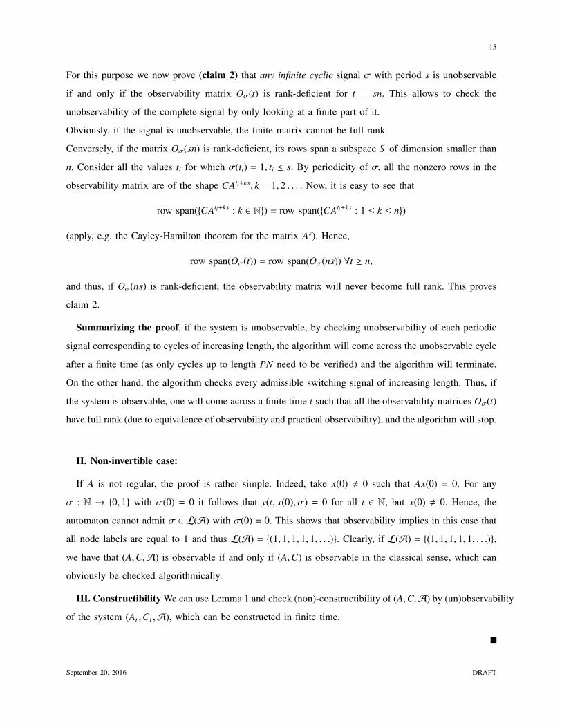
For this purpose we now prove (claim 2) that any infinite cyclic signal σ with period s is unobservable

if and only if the observability matrix Oσ(t) is rank-deficient for t = sn. This allows to check the

unobservability of the complete signal by only looking at a finite part of it.

Obviously, if the signal is unobservable, the finite matrix cannot be full rank.

Conversely, if the matrix Oσ(sn) is rank-deficient, its rows span a subspace S of dimension smaller than

n. Consider all the values ti for which σ(ti) = 1, ti ≤ s. By periodicity of σ, all the nonzero rows in the

observability matrix are of the shape CAti+ks, k = 1, 2 . . . . Now, it is easy to see that

row span({CAti+ks : k ∈ N}) = row span({CAti+ks : 1 ≤ k ≤ n})

(apply, e.g. the Cayley-Hamilton theorem for the matrix As). Hence,

row span(Oσ(t)) = row span(Oσ(ns)) ∀t ≥ n,

and thus, if Oσ(ns) is rank-deficient, the observability matrix will never become full rank. This proves

claim 2.

Summarizing the proof, if the system is unobservable, by checking unobservability of each periodic

signal corresponding to cycles of increasing length, the algorithm will come across the unobservable cycle

after a finite time (as only cycles up to length PN need to be verified) and the algorithm will terminate.

On the other hand, the algorithm checks every admissible switching signal of increasing length. Thus, if

the system is observable, one will come across a finite time t such that all the observability matrices Oσ(t)

have full rank (due to equivalence of observability and practical observability), and the algorithm will stop.

II. Non-invertible case:

If A is not regular, the proof is rather simple. Indeed, take x(0) , 0 such that Ax(0) = 0. For any

σ : N → {0, 1} with σ(0) = 0 it follows that y(t, x(0), σ) = 0 for all t ∈ N, but x(0) , 0. Hence, the

automaton cannot admit σ ∈ L(A) with σ(0) = 0. This shows that observability implies in this case that

all node labels are equal to 1 and thus L(A) = {(1, 1, 1, 1, 1, . . .)}. Clearly, if L(A) = {(1, 1, 1, 1, 1, . . .)},

we have that (A,C,A) is observable if and only if (A,C) is observable in the classical sense, which can

obviously be checked algorithmically.

III. Constructibility We can use Lemma 1 and check (non)-constructibility of (A,C,A) by (un)observability

of the system (Ar,Cr,A), which can be constructed in finite time.


16

Remark 2: Note that Skolem’s theorem not only allows to design an algorithm to decide observability

properties of a system (A,C,A), but it also allows to compute a priori the running time of (a slightly

modified version) of the algorithm, when one has computed an effective bound on the quantity P in

Skolem’s theorem. Indeed, one can simply run the second routine of the algorithm in this case as it

was shown in the proof above that the system is unobservable if and only if there is an ‘unobservable’

periodic signal based on a cycle (period) of length less than PN. Hence, one only has to check a finite

number of cycles (of length less than PN) to conclude on the observability/constructability or the absence

of it. This number is bounded a priori, and one can thus deduce an a priori bound on the computational

burden of the algorithm. However, as in some cases the computation of P is not so easy (or P might be

very large), the algorithm presented in the proof of the above theorem does not rely on the availability

of P by exploiting the two routines.

IV. Controllability results

In this section we address the following problem:

Problem 2: Given a constrained discrete-time switched linear system specified by the triple (A, B,A),

determine whether the system is (un)controllable, (un)reachable and (non-)0-controllable.

We will see that when the matrix A is regular, the problem can be seen as exactly the ‘dual’ of

the observability problem, and hence solved thanks to the technique described above. However, a bit

surprisingly, the duality does not hold when A is singular, and we also describe an algorithm for that

case in this section.

Lemma 3: Consider the system (A,C,A), and let S be a real Jordan form basis-transformation matrix

such that

S AS −1 =

Ar 0

0 As

, S B =

Br

Bs

, (8)

where Ar is regular, and As has only zero eigenvalues.

Then, (A,C,A) is 0-controllable if and only if (Ar, Br,A) is 0-controllable.

The proof of the above lemma follows using similar arguments as in the proof of Lemma 1 and is

therefore omitted here.

Just as in the observability problem, the controllability property is related with the space spanned by

the columns of a reachability matrix.


17

Definition 6: Given a data loss signal σ : N→ {0, 1}, we define the reachability matrix of the system

(A, B,A) at time t ∈ N by

Cσ(t) :=(Bσ(t − 1) ABσ(t − 2) . . . A(t−1)Bσ(0)

)∈ Rn×mt. (9)

Similarly, we also define the reachability matrix Cw(t) at time t ∈ N for finite signals (words) w :

{0, 1, . . . , r} → {0, 1} with r ∈ N≥t−1.

Note that for all t ∈ N and T ∈ N it holds that

Cσ(t + T ) = (Bσ(t + T − 1) ABσ(t + T − 2) . . . AT−1Bσ(t) ATCσ(t)

), (10)

which will turn out to be a useful identity.

Proposition 2: The system (A, B,A) is reachable if and only if for all σ ∈ L(A) there exists a T ∈ N

such that the reachability matrix Cσ(T ) is of rank n.

Proof: (Necessity) We proceed by contradiction. Suppose that there is a σ such that, for all t ∈ N,

the controllability matrix Cσ(t) is of rank smaller than n. Let us take x0 = 0 as in the definition of

reachability (Definition 4-(ii)). From (2) we have that

xx0,σ,u(t) = Cσ(t)ut−1, (11)

where ut−1 ∈ Rmt = col(u(t − 1), u(t − 2), . . . , u(0)) := [u(t − 1)> u(t − 2)> . . . u(0)>]>. Hence, the set of

reachable vectors at time t ∈ N is a strict linear subspace of Rn. Thus, the set of reachable points, which

is a countable union of these strict linear subspaces, cannot be equal to Rn.

(Sufficiency) Conversely, if for each σ there is a T ∈ N such that Cσ(T ) has full rank, then the system

is clearly reachable based on (11).

Proposition 3: The system (A, B,A) is controllable if and only if it is reachable. Moreover, reachability

implies 0-controllability and, in case A is invertible, the two notions are equivalent.

Proof: The ‘only if’ part is trivial. Let us prove the ‘if’ part of the first statement. Fix σ ∈ L(A), and

x0, x f ∈ Rn. By Proposition 2, since the system is reachable, there is a time t ∈ N such that rank(Cσ(t)) = n.

Equivalently,

Cσ(t)ut−1 = x f − At x0


18

has a solution ut−1 for any x0 and x f . The input signal u : N→ Rm starting with (u(0), u(1), . . . , u(t − 1))

transfers the initial state x0 to the final state x f at time t. Hence, the system (A, B,A) is controllable.

To prove the second statement, note first that since reachability implies controllability it also implies

0-controllability. To show the converse in case A invertible, note that given σ ∈ L(A) the set of all states

that can be steered to the origin in finite time is given by⋃

t∈N −A−tImCσ(t). From this identity it follows

that if the system is not reachable then there exists a σ such that ImCσ(t) is always a strict subspace of

Rn. Hence, the indicated union can never be Rn and the system is therefore not 0-controllable.

We will now prove various duality relationships to connect the observability and controllability con-

cepts. The following lemma will be useful in proving the duality relationships.

Lemma 4: Consider (A, B,A) with A regular and the set of admissible signals L(A) as in Definition 2.

Also, consider the setW(A) of finite words generated byA. The following two statements are equivalent:

I. There exists a signal σ ∈ L(A) such that for all t ∈ N the corresponding reachability matrix Cσ(t)

does not have full rank (i.e., the system is not reachable)

II. There exists a sequence {wi}i∈N≥1 of finite words wi ∈ W(A) of length i such that, for all i ∈ N≥1 the

corresponding reachability matrix Cwi(i) does not have full rank (i.e., the system is not practically

reachable).

Proof: The ‘I → II’-part is rather obvious since the successive prefixes of σ given by wi :=

(σ(0), . . . , σ(i − 1)) do the job as Cwi(i) = Cσ(i).

The proof of the other direction essentially comes from compactness of the language generated by

an automaton (with the standard topology on words), but we present here a self-contained proof for

clarity. Therefore, suppose that there is a sequence {wi}i∈N≥1 of finite words wi ∈ W(A) of length i such

that Cwi(i) does not have full rank. We now generate based on this sequence an infinite data loss signal

σ ∈ L(A) as follows. Starting with k = 0 we iteratively perform the following steps. Define at step

k ∈ N σ(k) such that there exists an infinite number of words in {wi}i∈N≥1 with the first k + 1 letters

equal to (σ(0), σ(1), . . . , σ(k)). This procedure can indefinitely be continued as at each step k ∈ N≥1

(σ(0), σ(1), . . . , σ(k − 1)) are given (by induction) and there are an infinite number of words in {wi}i∈N≥1

left with these first k letters (for k = 0 this holds trivially). This procedure generates an infinite word

σ : N→ {0, 1}. Due to (10) we obtain

Cwi(i) =


19

(Bwi(i − 1) ABwi(i − 2) . . . Ai−k−1Bwi(k) Ai−kCσ(k)

), (12)

which holds for all wi (i ∈ N≥k) that have the same first k letters as the constructed σ. Combining this

with Cwi(i) not having full rank and the regularity of A, it follows that for all k ∈ N the corresponding

observability matrix Cσ(k) does not have full rank, which concludes the proof.

We are now in position to establish the duality relationships for which we need the concept of a reverse

automaton.

Definition 7: Let an automaton A = (M, s) ∈ {0, 1}N×N×{0, 1}N be given as in Definition 1. The reverse

automaton is defined by Ar = (M>, s).

With this definition, for any w ∈ W(A) with length |w|, the time-reversed word rev(w) : {0, 1 . . . , |w| −

1} → {0, 1} given for t ∈ {0, 1 . . . , |w| − 1} by rev(w)(t) := w(|w| − t) satisfies rev(w) ∈ W(Ar). Hence, any

time-reversed finite word generated by A is a finite word of Ar and vice versa (as (Ar)r = A).

Proposition 4: If the system (A,C,A) is observable then the dual system (A>,C>,Ar) is controllable,

where Ar is the reverse automaton of A. Moreover, if A is a regular matrix, then the converse statement

also holds.

Proof: Let us suppose that the system (A,C,A) is observable and thus practically observable, and

select T as the bound in the definition of practical observability, i.e., Oσ(T ) has full rank for every

admissible signal σ of length T. Suppose now by contradiction that the system (A>,C>,Ar) is not

controllable. Hence, there is a finite signal w ∈ W(Ar) of length |w| = T such that the reachability

matrix

Cw(T ) =

(C>w(T − 1) . . . (A>)(T−1)C>w(0)

),

does not have full rank. Note that

Cw(T )> = Orev(w)(T ) (13)

and obviously rev(w) ∈ W(A). However, Orev(w)(T ) has full rank because of the practical observability

of system (A,C,A) with bound T , which is a contradiction and thus (A>,C>,Ar) is controllable.

To prove the second statement assume A regular and (A>,C>,Ar) is controllable. Suppose now by

contradiction that the system (A,C,A) is not observable. Then there exists a σ such that for all t ∈ N

Oσ(t) does not have full rank. By taking the successive prefixes of σ given wi = (σ(0), . . . , σ(i− 1)), we

obtain an infinite sequence of words wi ∈ W(A) of length |wi| = i, i ∈ N, such that the corresponding

observability matrix Owi(t) does not have full rank for all t ∈ N≤i. Using (13) and reversing the automaton,


20

we obtain rev(wi) ∈ W(Ar) such that Crev(wi)(i) does not have full rank. By Lemma 4, this implies the

existence of a signal σ such that Cσ(t) is rank-deficient for all t ∈ N and thus the system is not controllable.

Contradiction! Hence, (A,C,A) is observable.

From now on we call (A>,C>,Ar) the dual system of (A,C,A).

Proposition 5: The system (A,C,A) is constructible if and only if the dual system (A>,C>,Ar) is

0-controllable.

Proof: By Lemmas 1 and 4 we obtain (A,C,A) is constructible ⇔ (Ar,Cr,A) observable ⇔

((Ar)>, (Cr)>,Ar) reachable/controllable (using that Ar is regular). Since Ar is regular, reachability and

0-controllability are equivalent (combining Lemma 3 and Proposition 3).

Before putting all the pieces together, we are left with the controllability problem in the case where

A is singular.

Example 3: Take A = 0 and B = I with I the identity matrix of appropriate dimensions. We take

A as the automaton that has L(A) = {(1, 0, 1, 0, 1, 0, 1, . . .), (0, 1, 0, 1, 0, 1, 0, 1, . . .)} consisting of only

periodic data loss signals with period 2. Note that the dual system (A>, B>,Ar) is not observable and

in fact (0, 1, 0, 1, 0, 1, 0, 1, . . .) ∈ L(Ar) = L(A) leads to Oσ(t) = 0 not having full rank for all t ∈ N.

However, the original system (A, B,A) is controllable. Hence, in contrast with the LTI case without data

loss, in this case we do not have a complete duality result. Duality between controllability of a system

and observability of the dual system only holds when A is regular (or no data loss is allowed).

This example shows that, surprisingly, the duality relation does not hold in the case where A is not

regular. Hence, for deciding controllability in this case we must proceed differently than in the regular

case. By Lemma 3 one can separate the system into the regular part and the nilpotent part. Let us now

focus on a system where A is nilpotent and thus An = 0. Recall that in the observability case with A

nilpotent, the only case where observability can hold is the trivial case where no dropout is possible, see

the end of the proof of Theorem 2.

Proposition 6: Suppose that the matrix A is nilpotent. The controllability of the system (A, B,A) can

be checked algorithmically.

Proof: Let ` be the smallest k ∈ N≤n such that Ak = 0. Hence, by Proposition 2 we only have to

check the rank of all reachability matrices Cσ(t) with t ∈ N≤`, which is a finite check over all finite words

in W(A) with maximal length `.


21

The main result of this section is given next.

Theorem 3: Problem 2 is decidable in the sense that given a system specified by (A, B,A), there is

an algorithm that decides (un)controllability, (un)reachability and (non-)0-controllability of the system in

finite time.

Proof: If A is regular, one can check reachability by using Proposition 4 above, by checking

observability for the dual system. If A is singular, the system (A, B,A) is reachable if and only if both

the “regular” part (Ar, Br,A) and the “singular” part (As, Bs,A) are reachable (this can be seen most

easily by inspecting the structure in the reachability matrices based on the block diagonal structure in the

real Jordan form). The first system can be checked with Proposition 4 again, and the second one with

Proposition 6. Hence, reachability is decidable and thus controllability as well (recall that controllability

is equivalent to reachability (Proposition 3)).

Finally, 0-controllability (or the absence of it) can be checked by Proposition 5 (note that the dual of the

dual system is the original system) as constructibility is decidable due to Theorem 2.

Corollary 2: The system (A, B,A) is practically reachable (resp. practically controllable and practically

0-controllable) if and only if it is reachable (resp. controllable and 0-controllable).

Proof: In the spirit of Proposition 2 it is obvious that practical reachability is equivalent to the

existence of a finite T ∈ N such that for all σ ∈ L(A) it holds that for some t ∈ N≤T Cσ(t) has full rank.

From this it follows that (A, B,A) is practically reachable if and only if (Ar, Br,A) is practically reachable

by Lemma 4. Finally, due to nilpotence of As it is clear that (As, Bs,A) can only be reachable if and

only if it is practically reachable. This shows that reachability and practical reachability are equivalent

as reachability of a system is equivalent to reachability of its “regular” part (Ar, Br,A) and its “singular”

part (As, Bs,A).

Now, by the same arguments as in Proposition 3, practical controllability and practical reachability are

equivalent (and we already knew that controllability and reachability are equivalent).

Finally, due to nilpotence of As and the results in Lemma 3 it follows that (A, B,A) is practically

0-controllable ⇔ (Ar, Br,A) is practically 0-controllable ⇔ (Ar, Br,A) is 0-controllable ⇔ (A,C,A) is

0-controllable.

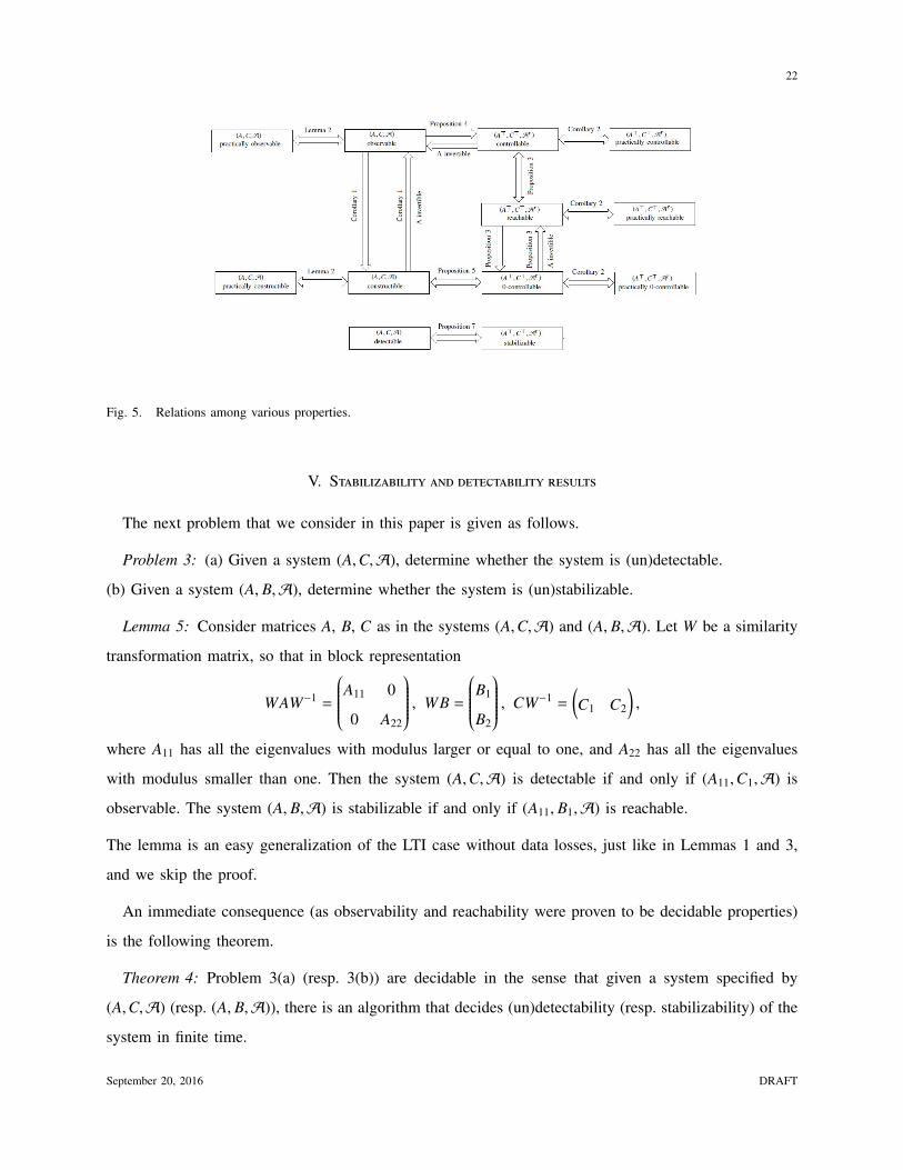
The relationships among various properties presented so far are summarized in Figure 5.


22

Fig. 5. Relations among various properties.

V. Stabilizability and detectability results

The next problem that we consider in this paper is given as follows.

Problem 3: (a) Given a system (A,C,A), determine whether the system is (un)detectable.

(b) Given a system (A, B,A), determine whether the system is (un)stabilizable.

Lemma 5: Consider matrices A, B, C as in the systems (A,C,A) and (A, B,A). Let W be a similarity

transformation matrix, so that in block representation

WAW−1 =

A11 0

0 A22

, WB =

B1

B2

, CW−1 =

(C1 C2

),

where A11 has all the eigenvalues with modulus larger or equal to one, and A22 has all the eigenvalues

with modulus smaller than one. Then the system (A,C,A) is detectable if and only if (A11,C1,A) is

observable. The system (A, B,A) is stabilizable if and only if (A11, B1,A) is reachable.

The lemma is an easy generalization of the LTI case without data losses, just like in Lemmas 1 and 3,

and we skip the proof.

An immediate consequence (as observability and reachability were proven to be decidable properties)

is the following theorem.

Theorem 4: Problem 3(a) (resp. 3(b)) are decidable in the sense that given a system specified by

(A,C,A) (resp. (A, B,A)), there is an algorithm that decides (un)detectability (resp. stabilizability) of the

system in finite time.


23

We also have the following duality result.

Proposition 7: The system (A,C,A) is detectable if and only if the dual system (A>,C>,Ar) is

stabilizable, where Ar is the reverse automaton of A.

Proof: First, (A,C,A) is detectable if and only if (A11,C1,A) is observable with the matrices A11

and C1 as in Lemma 5 (and transformation matrix W). Obviously, A11 is a regular matrix and thus

observability of (A11,C1,A) is equivalent to reachability of its dual system (A>11,C>1 ,A

r). As the latter is

equivalent to (A>,C>,Ar) being stabilizable based on Lemma 5 (with transformation matrix W−T ), the

proof is complete.

VI. Connections with systems subject to varying delays

In this section we make two links between our problem and a similar one, where the non-idealities in

the feedback loop incur time-varying delays, rather than pure packet losses. We mainly show that this

other model is a particular case of ours, and provide an algorithm to encapsulate any given controllability

problem with time varying delays as a controllability problem with packet losses as introduced in this

paper (Subsection VI-B). Then, in Subsection VI-C, we study a particular class of systems from the model

studied in this paper, namely, the systems with a bound on the maximal number of consecutive dropouts,

and we show how to model these particular systems as systems with varying delays. The interest of this

last result is that alternative algorithms, previously developed for systems with time-varying delays, can

then be used for this particular family of systems with packet dropouts.

A. Controllability under switching delays

We first briefly recall the framework of [14], [15], where the problem is to control a linear plant, when

the feedback loop is subject to time-varying delays. In [14], [15] the constraint on the combinatorial

structure of the delays is not given in terms of an automaton, but simply in terms of a set of natural

numbers, that represent delays, which can possibly be incurred on the feedback signal.

Definition 8: A system with varying delays is defined by a triple (A, B,D) with A ∈ Rn×n, B ∈ Rn×m

and D = {d1, d2, . . . , dN} ⊂ N is the set of admissible delays. Its dynamics is described by the equations

x(t + 1) = Ax(t) +∑

t′≤t,t′+d(t′)=t

Bu(t′) (14)

with

d : N→ D


24

being any arbitrary delay signal.

The meaning of Equation (14) is that at each time t′ = 1, 2, . . . , the control packet is subject to a certain

delay d(t′), which is determined by an exogenous switching signal d. The control packet u(t′) will impact

the state of the system not at time t′ + 1 as in a classical LTI system, but at time t′ + d(t′) + 1. If several

packets arrive at the actuator at the same time, it was arbitrated in [14], [15] that they are simply added.

The trajectory generated by the system (14) with initial state x(0) = x0, input sequence u : N→ Rm and

delay signal d : N→ D is denoted by xx0,d,u.

In the spirit of Definition 4 the following definition was introduced in [15].

Definition 9: We say that a system with varying delays described by the triple (A, B,D) is controllable

if for any delay signal d : N→ D, any initial state x0 ∈ Rn and any final state x f ∈ R

n, there is an input

signal u : N → Rm such that xx0,d,u(T ) = x f for some T ∈ N. In case the system is not controllable it is

said to be uncontrollable.

In this setting too, given a delay signal d : N→ D one can introduce the controllability matrix Cd(t) at

time t ∈ N.

Definition 10: Consider a system with time-varying delays (14). Given d : N → N we define the

controllability matrix at time t ∈ N as Cd(t) ∈ Rn×mt, whose i-th block-column (for all i ∈ N[1,t]) is given

by

• A(t−i−d(i−1))B, if i + d(i − 1) ≤ t;

• the zero column, if i + d(i − 1) > t.

The state of a system with varying delays as in (14) can be expressed thanks to its controllability

matrix as

xx0,σ,u(t) = At x0 + Cd(t)ut−1, (15)

where ut−1 ∈ Rmt is the column vector with all the inputs u(s), s = 0, . . . , t − 1. Again, controllability can

be related to the rank of the matrix Cd(t) as formalized next.

Proposition 8: [adapted from Proposition 4 in [15]] The delay system given by (A, B,D) is uncon-

trollable if and only if there is a delay signal d : N→ D such that for all t ∈ N it holds that Cd(t) does

not have full rank.

In order to best represent the link between the varying delays model and our packet dropouts model,

we introduce another useful concept: Given a delay signal d : N → N, we define the actuation signal


25

τd : N→ {0, 1} for t ∈ N by

τd(t) =

1, if there is a t′ ∈ N such that t′ + d(t′) = t,

0, otherwise.(16)

With this definition in place, the link between the two models is easy to express: it turns out that for all

d : N→ N and all t ∈ N, it holds that

ImCτd (t) = ImCd(t), (17)

where Cτd (t) is the Reachability matrix as defined in 6.

Proposition 8 gives us a characterization of controllable systems, but again not an algorithmic one.

Indeed it is not clear how to generate the signal σ as in the proposition, and even less clear how to

prove the inexistence of such an infinite-length signal. However, it is shown in [15] that this problem is

decidable and even more, that one can bound the time needed by the algorithm to answer the question.

B. The switching delays problem expressed as a dropout problem

In this subsection, we prove that the setting studied in this paper (where an automaton describes the

possible packet loss signals) is more general than the model with switching delays. Indeed, we take an

arbitrary controllability problem with switching delays, and we convert it to a controllability problem

with a dropout signal constrained by an automaton, as studied in this paper. Thus, the controllability test

introduced in this paper can be applied to the previously studied problem of controllability with varying

delays. However, the next example demonstrates that the proposed results in this paper apply to a much

richer class of automata than the ones produced by varying delays.

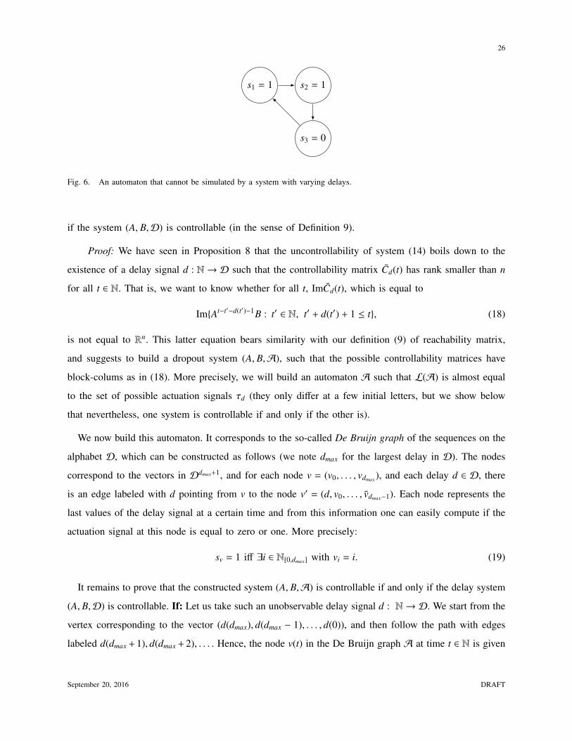
Example 4: Consider the automaton described by M =

0 1 0

0 0 1

1 0 0

and s =

1

1

0

, which is depicted in Fig-

ure 6. Clearly, L(A) = {(0, 1, 1, 0, 1, 1, 0, 1, 1, . . .), (1, 1, 0, 1, 1, 0, 1, 1, 0, 1, 1, . . .), (1, 0, 1, 1, 0, 1, 1, 0, 1, 1, . . .)}.

We claim that there is no system with varying delays that generates a language of actuation signals equal

to L(A). To see this, observe that if the delay signal is constant (i.e., the delay does not change with

time), the actuation signal is asymptotically equal to (1, 1, 1, . . . ), which is obviously not in L(A). Due

to this structure this automaton cannot be captured as a varying delay system.

Theorem 5: Let (A, B,D) represent a system as in Definition 10. One can construct an automaton A

with the following property: the system (A, B,A) is controllable (in the sense of Definition 4) if and only


26

s3 = 0

s1 = 1 s2 = 1

Fig. 6. An automaton that cannot be simulated by a system with varying delays.

if the system (A, B,D) is controllable (in the sense of Definition 9).

Proof: We have seen in Proposition 8 that the uncontrollability of system (14) boils down to the

existence of a delay signal d : N→ D such that the controllability matrix Cd(t) has rank smaller than n

for all t ∈ N. That is, we want to know whether for all t, ImCd(t), which is equal to

Im{At−t′−d(t′)−1B : t′ ∈ N, t′ + d(t′) + 1 ≤ t}, (18)

is not equal to Rn. This latter equation bears similarity with our definition (9) of reachability matrix,

and suggests to build a dropout system (A, B,A), such that the possible controllability matrices have

block-colums as in (18). More precisely, we will build an automaton A such that L(A) is almost equal

to the set of possible actuation signals τd (they only differ at a few initial letters, but we show below

that nevertheless, one system is controllable if and only if the other is).

We now build this automaton. It corresponds to the so-called De Bruijn graph of the sequences on the

alphabet D, which can be constructed as follows (we note dmax for the largest delay in D). The nodes

correspond to the vectors in Ddmax+1, and for each node v = (v0, . . . , vdmax), and each delay d ∈ D, there

is an edge labeled with d pointing from v to the node v′ = (d, v0, . . . , vdmax−1). Each node represents the

last values of the delay signal at a certain time and from this information one can easily compute if the

actuation signal at this node is equal to zero or one. More precisely:

sv = 1 iff ∃i ∈ N[0,dmax] with vi = i. (19)

It remains to prove that the constructed system (A, B,A) is controllable if and only if the delay system

(A, B,D) is controllable. If: Let us take such an unobservable delay signal d : N→ D. We start from the

vertex corresponding to the vector (d(dmax), d(dmax − 1), . . . , d(0)), and then follow the path with edges

labeled d(dmax + 1), d(dmax + 2), . . . . Hence, the node v(t) in the De Bruijn graph A at time t ∈ N is given


27

by v(t) = (d(t + dmax), d(t + dmax − 1), . . . , d(t)), and for any t ≥ 0, the corresponding packet loss signal is

given by σ(t) = τd(t + dmax) with τd the actuation signal corresponding to d (see (16)). Thus (see (19)),

σ(t) = 1⇔ ∃s ∈ N[t,dmax+t] : d(s) = t + dmax − s,

and from (9), the image of the reachability matrix Cσ(t) at an arbitrary time t ∈ N is included in

Im{At−t′−d(t′)−1+dmax B : t ≤ t′ ≤ t + dmax}. (20)

This set is exactly AdmaxIm(Cd(t)) with Cd(t) is the controllability matrix determining the controllability

of our system with varying delays (see (18)), which is never of rank n by hypothesis. Hence, we have

found a packet loss signal σ : N → {0, 1} in L(A) such that the reachability matrix has never full rank

and thus the system is not controllable.

Only if: Conversely, if there is a data loss signal σ ∈ L(A) such that the corresponding reachability

matrix Cσ(t) is never of rank n, the corresponding delay signal d obtained by the successive labels

di1 , . . . , dit on the edges of σ leads to a controllability matrix (see (18) again) with

ImCd(t) = Im{At−t′−d(t′)−1B : t′ ≥ 0, t − t′ − d(t′) − 1 ≥ 0}.

All these colums in this expression are colums of the reachability matrix (9) corresponding to the path

σ (see our definition of the labeling of the nodes of the automaton as in (19)), and so the matrix cannot

be of rank n.

We conclude this subsection by noting that this result gives an algorithm for deciding controllability of

systems with varying delays: Simply construct the automaton A described in the above proof, and decide

controllability of the system (A, B,A) with the techniques presented in this paper. We note, however,

that the alternative technique presented in [16] seems more advantageous, since: 1. It does not require to

build an auxiliary automaton, whose size can be exponential in the size of the initial problem and 2. in

[16], the total computational time of the algorithm is bounded w.r.t. the size of the initial problem, as a

function that does not depend on the numerical values of the entries of A. Thus, the algorithm developed

here might not be competitive in terms of computational time with the one previously introduced.

C. The particular case of maximal consecutive dropouts

As we have just seen in the previous subsection, the framework of this paper (where nonidealities are

represented by an automaton) is more general than systems with switching delays as in (14). However,


28

in this subsection we study the particular case where the automaton represents the constraint that the

actuation signal cannot contain more than N consecutive dropouts (like in Example 1). We show that in

this particular case, the controllability problem can be restated as a controllability problem with switching

delays. That is, the switching delays model encapsulates the constraint of maximal consecutive dropouts.

As a consequence, controllability with a maximum number of dropouts in a row can be solved with the

methodology developed there, for which a better bound on the running time of the algorithm is available.

However, we attract the attention of the reader on the fact that the techniques developed in [15] can

only be applied for the very particular case where the automaton is of the form in Fig. 3 (i.e., when

the constraint on the data loss signal is a bound on the number of consecutive losses). The case with an

arbitrary automaton is much more general and powerful (in terms of modeling of a data losses signal).

Theorem 6: Let us consider a system (A, B,A) with at most N consecutive dropouts (like defined in

Example 1) for some N ∈ N. The system (A, b,A) is controllable if and only if the delay system (A, B,D)

with D = {0, 1, . . . ,N}, is controllable.

Proof: First, observe that in both Definitions 6 and 10, the columns appearing in the controllability

matrix are uniquely defined by the packet loss signal σ (respectively the actuation signal τd), which

characterizes the set of times where B enters the controllability matrix.

Hence, if we can show that the language of actuation signals σ in the max-N-consecutive-dropouts

case, and the language of actuation signals τd induced by delay signals d : N→ D in the varying delay

case with D = {0, 1, . . . ,N} are the same, we have established the proof of the theorem. Indeed, there

would then exist an actuation signal σ which is uncontrollable in the max-N-consecutive-dropouts case

if and only if there exists an uncontrollable delay signal d : N→ D in the switching delays case.

To show that the languages are indeed equal, first take any signal σ : N → {0, 1} satisfying the

max-N-consecutive-dropouts constraint, that is

∀t ∈ N,∃t′ ∈ N[t,t+N] such that σ(t′) = 1. (21)

The signal σ is the same as τd corresponding to the delay signal d : N→ N given for t ∈ N by

d(t) = mint′≥t,σ(t′)=1

(t′ − t).

By (21), the above defined signal d(·) is admissible in the sense that d : N → D with D = {0, 1, . . . ,N},

as the right-hand side in the equation above is always smaller or equal to N.


29

Second, take a signal d : N→ {0, 1, . . . ,N}. It obviously incurs an actuation signal τd with at most N

zeros in a row, which is clearly contained in the set of admissible signals σ for the max-N-consecutive-

dropout case.

VII. Numerical example

Consider a discrete-time linear system subject to data losses (1) with

A =

−2 −13 9

−5 −10 9

−10 −11 12

and C =

(1 2 3

).

The observability matrix in the standard sense (with σ(t) = 1 for all t ∈ N) of the discrete-time linear

system is

O(A,C) =

C

CA

CA2

=

1 2 3

−42 −66 63

−216 513 −216

,the rank of which is 3. Consequently, the pair (A,C) is observable in the standard sense.

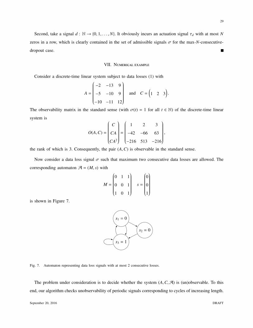
Now consider a data loss signal σ such that maximum two consecutive data losses are allowed. The

corresponding automaton A = (M, s) with

M =

0 1 1

0 0 1

1 0 1

s =

0

0

1

is shown in Figure 7.

s1 = 0

s2 = 0

s3 = 1

Fig. 7. Automaton representing data loss signals with at most 2 consecutive losses.

The problem under consideration is to decide whether the system (A,C,A) is (un)observable. To this

end, our algorithm checks unobservability of periodic signals corresponding to cycles of increasing length.


30

It is easy to verify (once the signal has been found) that the system (A,C,A) is unobservable under the

periodic data loss signal σ = (1, 0, 0, 1, 0, 0, 1, 0, 0, 1, . . .).

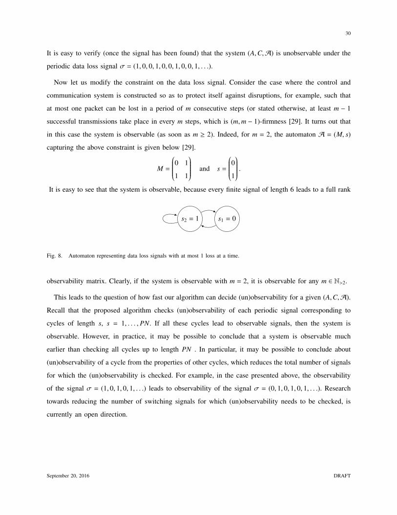
Now let us modify the constraint on the data loss signal. Consider the case where the control and

communication system is constructed so as to protect itself against disruptions, for example, such that

at most one packet can be lost in a period of m consecutive steps (or stated otherwise, at least m − 1

successful transmissions take place in every m steps, which is (m,m − 1)-firmness [29]. It turns out that

in this case the system is observable (as soon as m ≥ 2). Indeed, for m = 2, the automaton A = (M, s)

capturing the above constraint is given below [29].

M =

0 1

1 1

and s =

01 .

It is easy to see that the system is observable, because every finite signal of length 6 leads to a full rank

s1 = 0s2 = 1

Fig. 8. Automaton representing data loss signals with at most 1 loss at a time.

observability matrix. Clearly, if the system is observable with m = 2, it is observable for any m ∈ N>2.

This leads to the question of how fast our algorithm can decide (un)observability for a given (A,C,A).

Recall that the proposed algorithm checks (un)observability of each periodic signal corresponding to

cycles of length s, s = 1, . . . , PN. If all these cycles lead to observable signals, then the system is

observable. However, in practice, it may be possible to conclude that a system is observable much

earlier than checking all cycles up to length PN . In particular, it may be possible to conclude about

(un)observability of a cycle from the properties of other cycles, which reduces the total number of signals

for which the (un)observability is checked. For example, in the case presented above, the observability

of the signal σ = (1, 0, 1, 0, 1, . . .) leads to observability of the signal σ = (0, 1, 0, 1, 0, 1, . . .). Research

towards reducing the number of switching signals for which (un)observability needs to be checked, is

currently an open direction.


31

VIII. Conclusion

In this paper, our goal was to provide a theoretical analysis of how classical control-theoretic notions

are modified by typical non-idealities that are more and more present in modern control, as for instance in

wireless control networks. From a formal point of view, the problems we are trying to solve are extremely

hard, and even undecidable for arbitrary switched systems. However, our systems, while formally falling

in the class of switched systems, are not arbitrary, and their algebraic structure actually allows to retrieve

(part of) the powerful properties that are so useful for classical LTI systems. We have shown that packet

dropouts (under constraints represented by an automaton), while formally transforming the systems into

switched systems, keep enough algebraic structure so that fundamental questions like controllability or

observability can still be answered. As we have seen, the non-idealities under study in this paper are

quite general, and they even encapsulate previously studied models, like switching delays.

In further work, we plan to study models where observability and controllability interact in the same

feedback loop. Also, concerning the controllability problem, our work leaves natural open questions; for

instance, how to choose the control signal in real time? Indeed, remark that, in cases where our algorithm

returns a positive answer, we know that there exists a control signal that allows to stabilize the plant,

but nothing is said about how to chose the optimal signal. It is clear from our results how to chose this

signal a posteriori, i.e., once we know the dropout signal that effectively happened. However, in several

practical situations, it does not make sense to assume that the disruptions in the feedback loop are known

beforehand, and thus the controller has to ‘guess’ the optimal control value independently of the dropout

signal. From this point of view, our results can be viewed as necessary conditions for controllability (or

stabilizability, or...), which are not sufficient in the case of real-time control (note that the observability

problem does not suffer this limitation, since the essence of observability is that one recovers the state a

posteriori).

References

[1] M. Babaali and M. Egerstedt, Non-pathological sampling of switched system, IEEE Transactions on Automatic Control,

50 (2005), pp. 2102–2105.

[2] A. Bemporad, G. Ferrari-Trecate, andM. Morari, Observability and controllability of piecewise affine and hybrid systems,

IEEE Transactions on Automatic Control, 45 (2000), pp. 1864–1876.

[3] A. Bemporad, M. Heemels, and M. Johansson, eds., Networked control systems, vol. 406 of Lecture Notes in Control and

Information Sciences, Springer-Verlag, Berlin, 2010.

[4] V. D. Blondel and J. N. Tsitsiklis, Complexity of stability and controllability of elementary hybrid systems, Automatica,

35 (1999), pp. 479–489.


32

[5] M. K. Camlibel, Popov-Belevitch-Hautus type controllability tests for linear complementarity systems, Systems & Control

Letters, 56 (2007), pp. 381–387.

[6] M. K. Camlibel, W. P. M. H. Heemels, and J. M. Schumacher, Algebraic necessary and sufficient conditions for the

controllability of conewise linear systems, IEEE Transactions on Automatic Control, 53 (2008), pp. 762–774.

[7] X. Dai, A Gel’fand-type spectral radius formula and stability of linear constrained switching systems, Linear Algebra and

its Applications, 436 (2012), pp. 1099–1113.

[8] A. D’Innocenzo, M. D. Benedetto, and E. Serra, Fault tolerant control of multi-hop control networks, IEEE Transactions

on Automatic Control, 58 (2013), pp. 1377–1389.

[9] F. Felicioni, N. Jia, Y.-Q. Song, and F. Simonot-Lion, Impact of a (m,k)-firm data dropouts policy on the quality of control,

in IEEE International Workshop on Factory Communication Systems, 2006, pp. 353–359.

[10] T. Gommans, W. Heemels, N. Bauer, and N. van deWouw, Compensation-based control for lossy communication networks,

International Journal of Control, 86 (2013), pp. 1880–1897.

[11] N. Jia, Y.-Q. Song, and R.-Z. Lin, Analysis of networked control system with packet drops governed by (m, k)-firm constraint,

in International conference on fieldbus systems and their applications, 2005.

[12] R. Jungers andW. Heemels, Controllability of linear systems subject to packet losses, in Analysis and Design of Hybrid

Systems, 2015.

[13] R. Jungers, A. Kundu, andW. Heemels, On observability of networked control systems subject to packet losses, in Allerton

Conference on Communication, Control and Computing, 2015.

[14] R. M. Jungers, A. D’Innocenzo, andM. D. Di Benedetto, Feedback stabilization of dynamical systems with switched delays,

in IEEE Conference on Decision and Control, 2012.

[15] R. M. Jungers, A. D’Innocenzo, andM. D. Di Benedetto, Further results on controllability of linear systems with switching

delays, in IFAC World Congress, 2014.

[16] R. M. Jungers, A. D’Innocenzo, and M. D. Di Benedetto, Controllability of linear systems with switching delays, IEEE

Transactions on Automatic Control, 61 (2016), pp. 1117–1122.

[17] M. D. Kaba andM. K. Camlibel, Spectral conditions for the reachability of discrte-time conewise linear systems, in IEEE

Conference on Decision and Control, 2014.

[18] V. Kozyakin, The Berger–Wang formula for the markovian joint spectral radius, Linear Algebra and its Applications, 448

(2014), pp. 315–328.

[19] C. Lech, A note on recurring series, Arkiv for Matematik, 2 (1953), pp. 417–421.

[20] M. Pajic, S. Sundaram, G. J. Pappas, and R. Mangharam, The wireless control network: A new approach for control over

networks, IEEE Transactions on Automatic Control, 56 (2011), pp. 2305–2318.

[21] M. Philippe, R. Essick, G. Dullerud, and R. M. Jungers, Stability of discrete-time switching systems with constrained

switching sequences, Automatica, 72 (2015), pp. 242–250.

[22] L. Schenato, M. Franceschetti, K. Poolla, and S. S. Sastry, Foundations of control and estimation over lossy networks,

Proceedings of the IEEE, 95 (2007), pp. 163–187.

[23] B. Sinopoli, L. Schenato, M. Franceschetti, K. Poolla, M. Jordan, and S. Sastry, Kalman filtering with intermittent

observations, IEEE Transactions on Automatic Control, 49 (2004), pp. 1377–1389.

[24] T. Skolem, Ein verfahren zur behandlung gewisser exponentialer gleichungen und diophantischer gleichungen, Mathematica

Scandinavica, (1934), pp. 163–188.


33

[25] S. C. Smith and P. Seiler, Estimation with lossy measurement: jump estimators for jump systems, IEEE Transactions on

Automatic Control, 48 (2003), pp. 2163–2171.

[26] E. D. Sontag, Mathematical control theory, vol. 6 of Texts in Applied Mathematics, Springer-Verlag, New York, second ed.,

1998.

[27] Z. Sun, S. S. Ge, and T. H. Lee, Controllability and reachability criteria for switched linear systems, Automatica, 38 (2002),

pp. 775–786.

[28] M. Tabbara, D. Nesic, and A. R. Teel, Stability of wireless and wireline networked control systems, IEEE Transactions on

Automatic Control, 52 (2007), pp. 1615–1630.

[29] E. P. van Horssen, A. R. B. Behrouzin, D. Goswami, D. Antunes, T. Basten, andW. P. M. H. Heemels, Performance analysis

and controller improvement for linear systems with (m,k)-firm data losses, in European Control Conference, 2016.

[30] Y. Wang, N. Roohi, G. E. Dullerud, andM. Viswanathan, Stability of linear autonomous systems under regular switching

sequences, in IEEE Conference on Decision and Control, 2014.

[31] G. Xie and L. Wang, Controllability and stabilizability of switched linear-systems, Systems & Control Letters, 48 (2003),

pp. 135–155.


Documents

1 Observability and controllability analysis of linear systems … · · 2016-09-201 Observability and controllability analysis of linear systems subject to data losses Raphael