Observability and controllability of piecewise affine …moishi/eece571m/articles/BemporadMorari...1864 IEEE TRANSACTIONS ON AUTOMATIC CONTROL, VOL. 45, NO. 10, OCTOBER 2000 Observability

1864 IEEE TRANSACTIONS ON AUTOMATIC CONTROL, VOL. 45, NO. 10, OCTOBER 2000

Observability and Controllability of Piecewise Affineand Hybrid Systems

Alberto Bemporad, Giancarlo Ferrari-Trecate, and Manfred Morari

Abstract—In this paper, we prove, in a constructive way, theequivalence between piecewise affine systems and a broad classof hybrid systems described by interacting linear dynamics,automata, and propositional logic. By focusing our investigationon the former class, we show through counterexamples thatobservability and controllability properties cannot be easilydeduced from those of the component linear subsystems. Instead,we propose practical numerical tests based on mixed-integerlinear programming.

Index Terms—Controllability, hybrid systems, mixed-integerlinear programming, observability, piecewise affine systems,piecewise linear systems.

I. INTRODUCTION

I N recent years, both control and computer science have beenattracted byhybrid systems[1], [2], [23], [25], [26] because

they provide a unified framework for describing processesevolving according to continuous dynamics, discrete dynamics,and logic rules. The interest is mainly motivated by the largevariety of practical situations, for instance, real-time systems,where physical processes interact with digital controllers.

Several modeling formalisms have been developed to de-scribe hybrid systems, as reviewed in [24]. It is apparent thatthe tools for the analysis of hybrid systems strongly dependon the adopted mathematical description. Computer scientistshave extended automata theory totimed automata, where thecontinuous-time flow is modeled as , and further tolinearhybrid automata[1], where the dynamic is specified by thedifferential inclusion . On the other side, the controlcommunity started studying the so-calledhybrid dynamicalsystems[11] or hybrid automata[26] where the switchingbetween different dynamics is governed by a finite automaton.A special case where dynamic equations and switching rulesare linear functions of the state are the so-called piecewiseaffine (PWA) systems [33].

Recently, Bemporad and Morari [4] introduced a new classof hybrid systems called mixed logical dynamical (MLD) sys-tems. The justification for the MLD form is that it is capableof modeling a broad class of systems arising in many applica-tions: linear hybrid dynamical systems, hybrid automata, non-linear dynamic systems where the nonlinearity can be approx-

Manuscript received June 1, 1999; revised December 3, 1999. Recommendedby Associate Editor, S. Weiland. This work was supported by the Swiss NationalScience Foundation.

The authors are with the Institut für Automatik, ETH—Swiss Federal Insti-tute of Technology, CH 8092 Zürich, Switzerland (e-mail: bemporad, ferrari,[email protected]).

Publisher Item Identifier S 0018-9286(00)09445-9.

imated by a piecewise linear function, some classes of discreteevent systems, linear systems with constraints, etc. Examples ofreal-world applications that can be naturally modeled within theMLD framework are reported in [3]–[5].

MLD systems are formulated in discrete time. Although theeffects of sampling can be neglected in most applications, subtlephenomena such as Zeno behaviors cannot be captured in dis-crete time. On the other hand, although reformulating MLD sys-tems in continuous time would be quite easy from a theoreticalpoint of view, a discrete-time formulation allows developing nu-merically tractable schemes for solving complex problems, suchas control [4], state estimation and fault detection [3], [15], andformal verification of hybrid systems [5], [6]. For this reason,the analysis presented in this paper will be limited to discretetime.

The first result is to prove, in a constructive way, that MLDsystems are formally equivalent to PWA systems. This result al-lows extending all of the techniques developed for PWA modelsto the general MLD description of hybrid systems, thereforerendering the PWA framework a useful companion for investi-gating properties and designing algorithms. Although based ondifferent arguments, this importance has also been pointed outby Sontag [33], who highlights the equivalence between piece-wise linear (PWL) systems and interconnections of linear sys-tems and finite automata.

Piecewise affine systems are described by the state-spaceequations

for

(1)

where is a partition of the state+input set and, aresuitable constant vectors. Each subsystem defined by the 5-tuple

, is termed acomponentofthe PWA system (1). If and are null, system (1) is referredto as piecewise linear. From a complexity point of view, PWLand PWA systems are equivalent (, can be thought of asgenerated by integrators with no input).

PWA systems are sufficiently expressive to model a largenumber of physical processes, such as systems with static non-linearities (for instance, actuator saturation), and they can ap-proximate nonlinear dynamics with arbitrary accuracy via mul-tiple linearizations at different operating points.

Despite the fact that PWA models are just a composition oflinear time-invariant dynamic systems, their structural proper-ties such as observability, controllability, and stability are com-plex and articulated, as is typical of nonlinear systems.

0018–9286/00$10.00 © 2000 IEEE

BEMPORADet al.: OBSERVABILITY AND CONTROLLABILITY OF PIECEWISE SYSTEMS 1865

Consider, for instance, stability properties. Besides simple,but very conservative results such as finding one commonquadratic Lyapunov function for all of the components, re-searchers have started developing analysis and synthesis toolsfor PWA systems only very recently. By adopting piecewisequadratic Lyapunov functions, a computational approach basedon linear matrix inequalities has been proposed in [19] and [21]for stability analysis and control synthesis. Construction ofLyapunov functions for switched systems has also been tackledin [37]. For the general class of switched systems of the form

, , an extension of the Lyapunov criterionbased on multiple Lyapunov functions was introduced in [9]and [10]. Blondel and Tsitsiklis [8] showed that the stabilityof autonomous PWL systems is hard to verify (i.e., ingeneral, the stability of a PWL system cannot be assessedby a polynomial-time algorithm, unless ), even inthe simple case of two component subsystems. Several globalproperties (such as global convergence and asymptotic stability)of PWA systems have been recently shown undecidable in [7].

The research into stability criteria for PWL systems has beenmotivated by the fact that the stability of each component sub-system is not enough to guarantee stability of a PWL system(and vice versa). Branicky [10] gives an example where stablesubsystems are suitably combined to generate an unstable PWLsystem. Stable systems constructed from unstable ones havebeen reported in [36]. These examples point out that restrictionson the switching have to be imposed in order to prove that aPWL composition of stable components remains stable.

Very little research focused on the observability and control-lability properties of hybrid systems, apart from contributionslimited to the field of timed automata [1], [20], [23] and the pio-neering work of Sontag [30] for PWL systems. Needless to say,these concepts are fundamental for understandingif and howwell a state observer and a controller for a hybrid system canbe designed. For instance, observability properties were directlyexploited for designing convergent state estimation schemes forhybrid systems in [15].

Controllability and observability properties have been inves-tigated in [14] and [18] for linear time-varying systems, and inparticular for the so-called class of piecewise constant systems(where the matrices in the state-space representation are piece-wise constant functions of time). Although in principle appli-cable, these results do not allow one to catch the peculiarities ofPWA systems.

General questions of the hardness of the controllabilityof nonlinear systems were addressed by Sontag [32]. Followinghis earlier results [30], [31], Sontag [33] analyzes the com-putational complexity of the observability and controllabilityof PWA systems through arguments based on the languageof piecewise linear algebra. The author proves that observ-ability/controllability is complete over finite time, and isundecidable over infinite time (i.e., in general, cannot be solvedin finite time by means of any algorithm). Using a differentrationale, the same result was derived in [8].

In this paper, we provide two main contributions to the anal-ysis of the controllability and observability of hybrid and PWAsystems: 1) we show the reader that observability and control-

lability properties can be very complex; we present a numberof counterexamples that rule out obvious conjectures about in-heriting observability/controllability properties from the com-posing linear subsystems1; and 2) we provide observability andcontrollability tests based onlinear and mixed-integer linearprograms(MILP).

II. M IXED LOGICAL DYNAMICAL (MLD) SYSTEMS

The mixed logical dynamical (MLD) form was introducedin [4], based on the idea of transforming logic relations intomixed-integer linear inequalities [28], [35]. It is a modelingframework that allows the description of various classes of sys-tems, like systems with mixed discrete/continuous inputs andstates, automata driven by events on continuous dynamics, sys-tems with qualitative outputs, and PWA systems. The ability toinclude constraints, constraint prioritization, and heuristics aug-ments the expressiveness and generality of the MLD framework.The general MLD form is

(2a)

(2b)

(2c)

where are the continuous and binary states,are the inputs, are the

outputs, and , represent auxiliary binaryand continuous variables, respectively. All constraints on state,input, , and variables are summarized in the inequality (2c).Although the description (2) seems to be linear, nonlinearityis concentrated and hidden in the integrality constraints overbinary variables.

We assume that system (2) iscompletely well posed[4],which in words means that, for all within a bounded set,the variables are uniquely determined, i.e., there existfunctions , such that, at each time, ,

.2 This allows assuming thatand are uniquely defined once , are given, andtherefore that and trajectories exist and are uniquelydetermined by the initial state and input trajectory .

The auxiliary variables are introduced when transformingpropositional logic into linear inequalities. We briefly reviewhere these translation techniques, and refer the reader to [4] fora detailed exposition.

By following standard notation [12], [35], [38], [39], weadopt capital letters to represent statements, e.g., “ ”or “temperature is hot.” is commonly referred to as aliteral, and has atruth value of either “T” (true) or “F”(false). Boolean algebra enables statements to be combinedin compound statements by means ofconnectives:“ ” (and),“ ” (or), “ ” (not), “ ” (implies), “ ” (if and only if), “ ”(exclusive or). Connectives satisfy several properties (see, e.g.,[13]), which can be used to transform compound statements

1We thank one of the anonymous reviewers for pointing out that similar coun-terexamples were orally presented by Leonid Gurvits.

2A more general definition of well posedness, where only the components of� andz entering (2a)–(2b) are required to be unique, is given in [4].


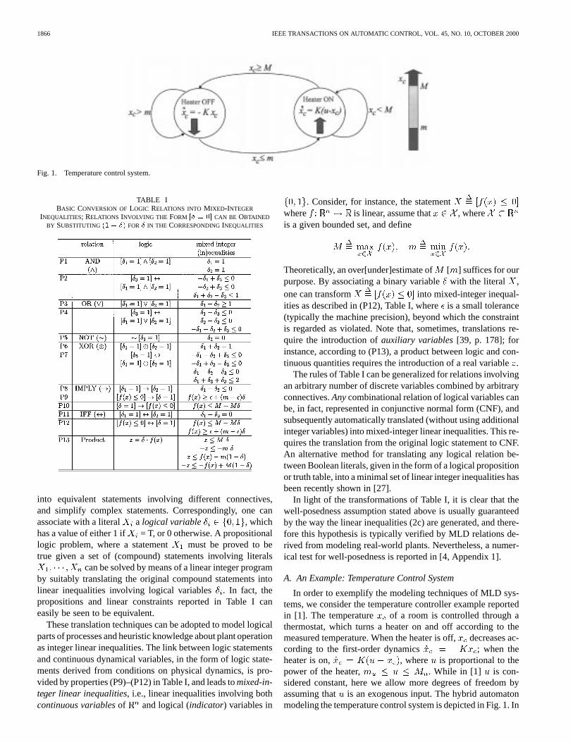
Fig. 1. Temperature control system.

TABLE IBASIC CONVERSION OFLOGIC RELATIONS INTO MIXED-INTEGER

INEQUALITIES; RELATIONS INVOLVING THE FORM [� = 0] CAN BE OBTAINED

BY SUBSTITUTING (1� �) FOR� IN THE CORRESPONDINGINEQUALITIES

into equivalent statements involving different connectives,and simplify complex statements. Correspondingly, one canassociate with a literal a logical variable , whichhas a value of either 1 if = T, or 0 otherwise. A propositionallogic problem, where a statement must be proved to betrue given a set of (compound) statements involving literals

can be solved by means of a linear integer programby suitably translating the original compound statements intolinear inequalities involving logical variables. In fact, thepropositions and linear constraints reported in Table I caneasily be seen to be equivalent.

These translation techniques can be adopted to model logicalparts of processes and heuristic knowledge about plant operationas integer linear inequalities. The link between logic statementsand continuous dynamical variables, in the form of logic state-ments derived from conditions on physical dynamics, is pro-vided by properties (P9)–(P12) in Table I, and leads tomixed-in-teger linear inequalities, i.e., linear inequalities involving bothcontinuous variablesof and logical (indicator) variables in

. Consider, for instance, the statementwhere is linear, assume that , whereis a given bounded set, and define

Theoretically, an over[under]estimate of [ ] suffices for ourpurpose. By associating a binary variablewith the literal ,one can transform into mixed-integer inequal-ities as described in (P12), Table I, whereis a small tolerance(typically the machine precision), beyond which the constraintis regarded as violated. Note that, sometimes, translations re-quire the introduction ofauxiliary variables[39, p. 178]; forinstance, according to (P13), a product between logic and con-tinuous quantities requires the introduction of a real variable.

The rules of Table I can be generalized for relations involvingan arbitrary number of discrete variables combined by arbitraryconnectives.Anycombinational relation of logical variables canbe, in fact, represented in conjunctive normal form (CNF), andsubsequently automatically translated (without using additionalinteger variables) into mixed-integer linear inequalities. This re-quires the translation from the original logic statement to CNF.An alternative method for translating any logical relation be-tween Boolean literals, given in the form of a logical propositionor truth table, into a minimal set of linear integer inequalities hasbeen recently shown in [27].

In light of the transformations of Table I, it is clear that thewell-posedness assumption stated above is usually guaranteedby the way the linear inequalities (2c) are generated, and there-fore this hypothesis is typically verified by MLD relations de-rived from modeling real-world plants. Nevertheless, a numer-ical test for well-posedness is reported in [4, Appendix 1].

A. An Example: Temperature Control System

In order to exemplify the modeling techniques of MLD sys-tems, we consider the temperature controller example reportedin [1]. The temperature of a room is controlled through athermostat, which turns a heater on and off according to themeasured temperature. When the heater is off,decreases ac-cording to the first-order dynamics ; when theheater is on, , where is proportional to thepower of the heater, . While in [1] is con-sidered constant, here we allow more degrees of freedom byassuming that is an exogenous input. The hybrid automatonmodeling the temperature control system is depicted in Fig. 1. In


order to translate the automaton into the MLD form (2), we dis-cretize the continuous dynamics with sampling time, namely,

if heater OFF

if heater ON(3)

where . Then, we introduce the auxiliary binary vari-ables

(4a)

(4b)

which take into account the crossing of the guard lines (obvi-ously, ). Equations (4a)–(4b) can be transformed intomixed-integer linear inequalities by using (P12) in Table I (weassume that a lower bound and an upper bound overare known).

A logic state is needed to store the status of the heater,and evolves according to the equation

(5)

where

(6a)

(6b)

(6c)

and

(7)

(although is redundant here, the reason for introducing it willbe clear in Section III).

As and cannot be 1 at the same time, we include theconstraint

(8)

Equations (6a) and (6b) are translated into inequalities ac-cording to (P8). Equation (6c) is equivalent to

(9)

Although (9) can be immediately verified by inspection, it hasbeen obtained by applying the technique described in [27] totransform general propositional logic statements into mixed-in-teger linear inequalities through polyhedral computation.

The dynamics (3) can be equivalently rewritten as

(10)

Because of the product involving and , we introducethe auxiliary continuous variable ,which can be transformed into mixed-integer linear inequalities,according to (P13) in Table I.

The transformations above can be summarized in the fol-lowing MLD representation of the temperature control system:

(11a)

(11b)

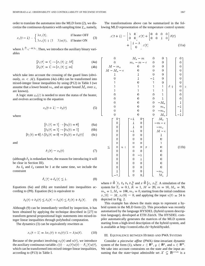
where and . A simulation of thesystem for , , , , ,

, , , starting from the initial condition, , and applying the input is

depicted in Fig. 2.This example has shown the main steps to represent a hy-

brid system in the MLD form (2). This procedure was recentlyautomatized by the language HYSDEL (hybrid system descrip-tion language), developed at ETH Zürich. The HYSDEL com-piler automatically generates the matrices of the MLD systemstarting from a high-level description of the hybrid system, andis available at http://control.ethz.ch/~hybrid/hysdel.

III. EQUIVALENCE BETWEENHYBRID AND PWA SYSTEMS

Consider apiecewise affine(PWA) time-invariant dynamicsystem of the form (1), where , , and .We take into account constraints on the state and the input as-suming that the state+input admissible set is a


Fig. 2. Simulation of the temperature control system. The different regions where PWA component subsystems are active are depicted with different textures.

TABLE IIVALID COMBINATIONS [� � � � ] AND RESPECTIVEFUNCTIONS

z = G(x; u)

convex and bounded polyhedron. Moreover, we suppose that,forms a polyhedral partition3 of .

A frequent representation of (1) arises in gain scheduling,where the linear model (and, consequently, the controller) isswitched among a finite set of models, according to changes ofthe operating conditions.

PWA systems can be represented in the MLD form (2).The translation consists of defining logical variables

and imposing the exclusive-orcondition .Fordetails, the reader is referred to [4].

Conversely, we will show in Proposition 1 that every MLDmodel (2) is equivalent to a PWA system.

Before stating this general conversion result, we consideragain the temperature control system of Section II-A. It is easyto check from (6a)–(9) that only the combinationsreported in Table II are allowed. The corresponding relationsbetween and , are also reported in Table II.

3Each setX is a (not necessarily closed) convex polyhedron s.t.X X =;, 8 i 6= j, X = X .

As the switching is governed by changes of vector , it isintuitive that the number of regions in which the state spaceis partitioned coincides with the number of validcombinations(i.e., six). To see this, consider, for example, . Thisgives , and, by substituting in (11b), the correspondingregion is defined by the inequalities

(12)

where redundant constraints have been eliminated by using stan-dard procedures based on linear programming. Moreover, from(11a) and , it follows that, in the region defined by (12),the state-update equations are

(13)

In Fig. 2, the different regions where PWA component subsys-tems are active are depicted by different textures.

Proposition 1: Consider generic trajectories , ,of an MLD system (2). Then there exist a polyhedral partition

of the state input set

s.t. (2c) holds for some


and 5-tuples , , , , , , such that ,, satisfy (1).Proof: In order to simplify the proof, without loss of gen-

erality, we assume that the logical componentsof are alsoauxiliary variables, i.e., such that .This is not a restrictive assumption, as typically the state tran-sition of logical states derives from a logic predicate involvingliterals associated with components of and , and thelatter can be expressed again as additional auxiliary variables bysimply adding the constraints ,in (2c).

By the well posedness of system (2), given , , thevector is uniquely defined, namely, .Moreover, it only takes a value within a set of (at most)values (corresponding to all possible 0–1 combinations). Letbe the number of valid combinations, i.e., the number of all dif-ferent vectors satisfying constraints (2c) for some

, , . The idea is to partition the state+input spaceby grouping in regions all corresponding to the samebinary vector . Let us fix . The in-equalities (2c) define a polyhedronin . By the wellposedness of , given a pair , , there exists only onevalue satisfying (2c), namely, .As all of the inequalities (2c) are linear, is an affine function,namely,

(14)

and is a polyhedral set of dimension less than orequal to (for instance, if , , , wouldbe a segment in ). By substituting (14) in (2a) and (2b), weobtain

which, by suitable choice of , , , , , ,corresponds to (1) for

Remark 1: We stress the fact that the proof is based on aconstructive argument. In fact, as was done in the temperaturecontrol system example, information on the description of thesystem can be used to derive (14), either from direct insight orautomatically from the inequalities (2c).

Remark 2: From a computational point of view, bothforms (1) and (2) have advantages. As in the case of lineartime-varying systems, the former allows expressing the evolu-tion of the system in a very compact way, for instance, whendealing with reach-set computation [6] (i.e., the computation ofthe set of states which are reachable from a given set of initialconditions). On the other hand, the latter allows inference,

e.g., in a switching detection problem, namely, the problem ofdetermining all possible new regions’s entered by a set ofstate vectors at the next time step. While the PWA form wouldbe required for enumerating and checking for the nonemptinessof the intersections of the updated set with all of the regions

, , the MLD form instead can be convenientlyexploited to solve the problem through mixed-integer linearoptimization involving , as free variables [6]. This in-directly moves the inference problem to the branch-and-boundstrategy of the MILP solver.

IV. OBSERVABILITY

In this section, we consider observability of MLD systems (2)or, equivalently, PWA systems in view of Proposition 1.

Denote by the output evolution at time startingfrom the initial condition and driven by the input ,

. We extend the definition of observability given in[22] and [29] to nonautonomous hybrid systems of the form (2).

Definition 1: Let be a set of initialstates, and let be a set of inputs. TheMLD system (2) isincrementally observable in steps onuniformly with respect to or simplyincrementally observableif there exist two norms (on ) and (on )and a positive scalar such that and inputsequences :

(15)

Remark 3: When including the input in the definition ofobservability of nonlinear systems, some authors prefer askingthat “ ” (an input sequence such that ) in-stead of “ .” As typically an observer is used together witha controller, we have opted for the latter. In fact, in this situ-ation, the output of the controller is not a sequence which isknowna priori, and therefore observability should be requiredwith respect toall possible input commands generated by thecontroller. Moreover, the class of such commands is usuallyspecified by the control system design, for instance, directly bylimits on actuators.

Remark 4: The parameters and appearing in Definition1 admit a practical interpretation. The scalarcan be viewedas an observability measure4 for an incrementally observablesystem. For fixed initial states and , the larger , the moredifferent the trajectories , [from now on,we will write in short , ]. Hence, in practice, onewould fix a minimum observability level and require that

. If this condition is not fulfilled, we classify thesystem aspractically unobservable. Practical unobservabilityalso arises if Definition 1 is satisfied only for large. There-fore, it is sensible to fix an upper bound on , and definean MLD system as practically observable when it satisfies Def-inition 1 with .

Condition (15) is simply anincremental distinguishabilitycondition, i.e., it states that different initial states always give

4More precisely, one should use~w = supfw > 0 s.t. (15) holdsg as theobservability measure.


different outputs, independently of the applied input. However,although , in principle, there might be a compo-nent of which is not observable. But this cannot be true. In fact,in this case, one could take two initial states such that the ob-servable component is the same, which implies ,

, thus violating Definition 1. In conclusion, the notionsof incremental distinguishability and incremental observabilitycoincide.

For bounded sets , it is easy to verify that the termin Definition 1 could be substituted by a

more general function (see [22] for thedefinition of the class) such that is lower and upperLipschitz, i.e., there exist positive constants, such that

. Therefore, we can conclude thatDefinition 1 is not much more restrictive than thepropertygiven in [22].

A. Observability Counterexamples for PWA Systems

Definition 1 was formulated for the general class of hybridsystems described by the MLD form (2) or, equivalently, thePWA form (1). One might expect to exploit the structure of PWAsystems to derive results about observability similar to thoseholding for linear systems. Below we show some counterexam-ples which undermine these hopes, even in the simpler case ofautonomous PWL systems.

We first show that, in general, for PWL systems, the timeof observability has no relation to the order of each sub-system, and therefore, if a PWL system is incrementally observ-able, nothing can be said, in general, about the minimumsuchthat Definition 1 holds.

Then, we show examples where the observability propertiesof a PWL system cannot be directly inferred from the observ-ability properties of its linear subsystems. In fact, we will showthat unobservable subsystems can be composed to build an ob-servable PWL system, and vice versa, that the composition ofobservable subsystems can become unobservable.

1) A PWL System Incrementally Observable withArbi-trarily Large: Consider the following system:

if

otherwise

(16)

where is fixed, and set

(17)

Then , where

and denotes the least upper integer. Moreover,, and therefore two initial states

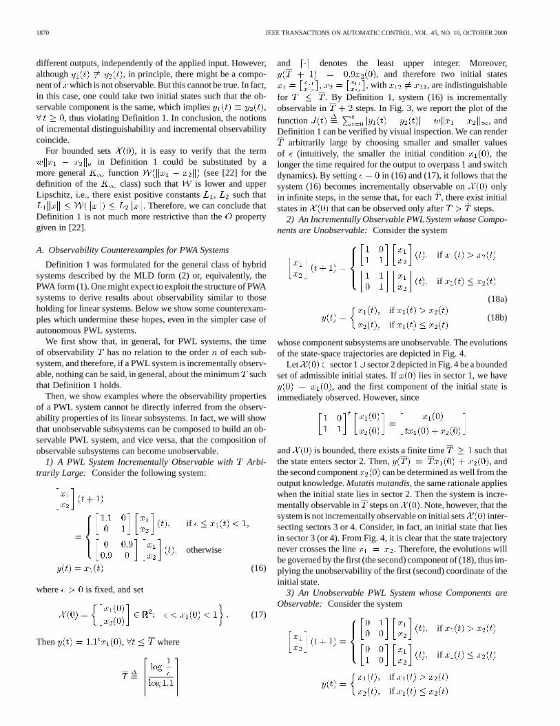
, , with , are indistinguishablefor . By Definition 1, system (16) is incrementallyobservable in steps. In Fig. 3, we report the plot of thefunction , andDefinition 1 can be verified by visual inspection. We can render

arbitrarily large by choosing smaller and smaller valuesof (intuitively, the smaller the initial condition , thelonger the time required for the output to overpass 1 and switchdynamics). By setting in (16) and (17), it follows that thesystem (16) becomes incrementally observable on onlyin infinite steps, in the sense that, for each, there exist initialstates in that can be observed only after steps.

2) An Incrementally Observable PWL System whose Compo-nents are Unobservable:Consider the system

if

if

(18a)if

if(18b)

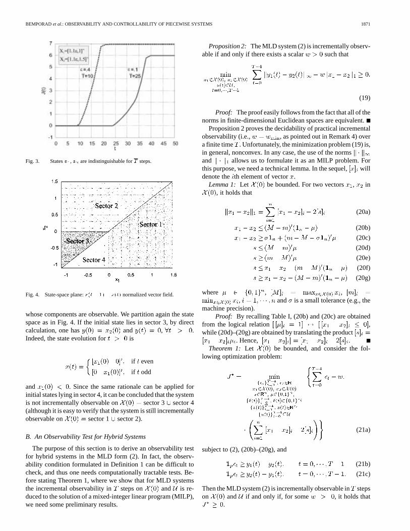
whose component subsystems are unobservable. The evolutionsof the state-space trajectories are depicted in Fig. 4.

Let sector 1 sector 2 depicted in Fig. 4 be a boundedset of admissible initial states. If lies in sector 1, we have

, and the first component of the initial state isimmediately observed. However, since

and is bounded, there exists a finite time such thatthe state enters sector 2. Then, , andthe second component can be determined as well from theoutput knowledge.Mutatis mutandis, the same rationale applieswhen the initial state lies in sector 2. Then the system is incre-mentally observable in steps on . Note, however, that thesystem is not incrementally observable on initial sets inter-secting sectors 3 or 4. Consider, in fact, an initial state that liesin sector 3 (or 4). From Fig. 4, it is clear that the state trajectorynever crosses the line . Therefore, the evolutions willbe governed by the first (the second) component of (18), thus im-plying the unobservability of the first (second) coordinate of theinitial state.

3) An Unobservable PWL System whose Components areObservable: Consider the system

if

if

if

if


Fig. 3. Statesx , x are indistinguishable forT steps.

Fig. 4. State-space plane:x(t+ 1)� x(t) normalized vector field.

whose components are observable. We partition again the statespace as in Fig. 4. If the initial state lies in sector 3, by directcalculation, one has and , .Indeed, the state evolution for is

if even

if odd

and . Since the same rationale can be applied forinitial states lying in sector 4, it can be concluded that the systemis not incrementally observable on sector 3 sector 4(although it is easy to verify that the system is still incrementallyobservable on sector 1 sector 2).

B. An Observability Test for Hybrid Systems

The purpose of this section is to derive an observability testfor hybrid systems in the MLD form (2). In fact, the observ-ability condition formulated in Definition 1 can be difficult tocheck, and thus one needs computationally tractable tests. Be-fore stating Theorem 1, where we show that for MLD systemsthe incremental observability in steps on and is re-duced to the solution of a mixed-integer linear program (MILP),we need some preliminary results.

Proposition 2: The MLD system (2) is incrementally observ-able if and only if there exists a scalar such that

(19)

Proof: The proof easily follows from the fact that all of thenorms in finite-dimensional Euclidean spaces are equivalent.

Proposition 2 proves the decidability of practical incrementalobservability (i.e., , as pointed out in Remark 4) overa finite time . Unfortunately, the minimization problem (19) is,in general, nonconvex. In any case, the use of the normsand allows us to formulate it as an MILP problem. Forthis purpose, we need a technical lemma. In the sequel,willdenote theth element of vector .

Lemma 1: Let be bounded. For two vectors , in, it holds that

(20a)

(20b)

(20c)

(20d)

(20e)

(20f)

(20g)

where , ,, and is a small tolerance (e.g., the

machine precision).Proof: By recalling Table I, (20b) and (20c) are obtained

from the logical relation ,while (20d)–(20g) are obtained by translating the product

. Hence, .Theorem 1: Let be bounded, and consider the fol-

lowing optimization problem:

(21a)

subject to (2), (20b)–(20g), and

(21b)

(21c)

Then the MLD system (2) is incrementally observable instepson and if and only if, for some , it holds that

.


Proof: We start by proving necessity. Inequalities (21b)and (21c) imply that

(22)

By Lemma 1,

(23)

Then, combining (22) and (23),

(24)

In view of Proposition 2, the condition follows from theincremental observability of system (2).

To show sufficiency, assume and consider

(25)

subject to constraints (2), and let, denote the initial statesthat minimize (25). The variables , , and defined as

if

if

are feasible for problem (21a). Thus, by optimality,, which proves incremental observability.Theorem 1 is also helpful for designing an algorithm that

checks the practical observability of an MLD system (see Re-mark 4. The procedure is summarized in the following steps.

Algorithm 1:1) Choose and (see Remark 4).2) Set and .3) Solve the MILP (21a).4) If , stop: the system is

(practically) observable.5) If , increase .6) If , stop: the system is

practically unobservable.7) Go to step 3).

Remark 5: When the sets , are polytopes, the opti-mization problem (21) becomes an MILP incontinuous variables and integer variables. Itis well known that, with the exception of particular structures,MILP’s involving 0–1 variables are complete, which meansthat, in the worst case, the solution time grows exponentially

with the number of integer variables [28]. Despite this combi-natorial nature, several algorithmic approaches have been pro-posed and applied successfully to medium- and large-size ap-plication problems [17], andbranch-and-boundmethods wereshown to be extremely successful.

In case the observability horizon becomes large, solvingsuch an optimization can become computationally intractable.As noted in the Introduction, this has to be expected because ofthe -complete nature of the observability problem itself overa finite horizon [33]. Consider, for instance, the autonomous case(no input). By looking more closely at the MILP (21a), the mainreason for the complexity is the presence of integer variables

. Indeed, determining the optimal sequencecorresponds to finding the sequence of the switching of lineardynamics, which leads to the worst case for observability.

Nevertheless, we now propose an algorithm which, althoughstill exponential in the worst case, is very efficient on average.In fact, the difficulty caused by the (possibly huge) number ofcombinations of binary variables ( , as pointed outin Remark 5) will be avoided in general by exploiting the equiv-alent PWA structure of hybrid systems.

C. An Efficient Observability Test for Hybrid Systems

We describe here a procedure to check the observability ofPWA systems that reduces the computational complexity of Al-gorithm 1. We adopt tools developed forformal verificationof hybrid systems [5], [6] where, basically, a set-reachabilityproblem is solved through the exploration of all possible evolu-tions of the hybrid system from the set of initial states .

The main advantage of adopting verification schemes is thatthey can exploit the PWA dynamics (1) when exploring thetemporal evolution from the initial set . More specifically,in the MILP problem (21a), the task of deciding in whichorder to explore the possible combinations of integer vectors

is assigned to the numerical solver. Clearly,most of the combinations will not be compatible with theconstraints (2c). Next Algorithm 2 avoids considering theseinadmissible combinations.

Let be a list of subsets , i.e., ,and let # denote its length (by convention, # iff). When a new set is added or removed to the list, we write,

respectively, or . Finally, denote thestate trajectory generated from the initial condition . Forthe sake of simplicity, we consider a formulation for autonomousPWA systems, although the presence of inputs can be taken intoaccount by adapting the verification algorithm proposed in [6].

Algorithm 2:1) Set and .2) For : if ,

then .3) While :

3.1) for , : solve


3.2) for : if ,, then

3.3) if , STOP: the PWL system ispractically incrementallyobservable in steps

3.4) set3.5) for

3.5.1) let be the index such that

3.5.2) for : if,

3.6) increase3.7) if , STOP: the system is

practically unobservable3.8) .

Algorithm 2 computes the evolution from the initial setin order to explore all possible state trajectories . In anycase, since after steps there may exist some subsets ofwhose elements can be observed (i.e., distinguished from theother states in in steps), the algorithm avoids furtherpropagating such states. More precisely, at step 3.1, the set

collects the evolution of all of the initial states that arenot observable in steps. Then, the algorithm checks if all ofthe initial states such that are distinguish-able from the initial states satisfying .This is done in step 3.1 by computing because, analogouslyto (19), the distinguishability condition corresponds to .In particular, if , , the subset of initialstates evolving in is observable (in steps). Then, there isno need to further consider the evolution of the set, and itis removed from the list (step 3.2). It is also apparent that thepractical incremental observability of the PWA system coincideswith the condition (step 3.3).

The one-step evolution of the sets is performed in step 3.4.Note that, from steps 2 and 3.5.2, it follows that each setbelongs at most to a single region of the state space. Thisensures that the index(step 3.5.1) is always well defined and,in step 3.5.2, every set evolves according the state equationof the region which it belongs to. Moreover, if the set

intersects regions, it is split into new sets (each onebelonging only to a single region ) that are then added to theupdated list .

Algorithm 2 is more suitable for implementation when theinitial set is a bounded polyhedron. In this case, by meansof the update step 3.5.2, every set is a polytope as well.Moreover, the minimization in step 3.1 becomes a mixed-integerlinear program. Actually, following the rationale of Theorem 1,it is easy to prove that

(26)

subject to (1), (20b)–(20g), (21b), and (21c). Note that eachMILP problem (26) involves only integer variables versus the

required for problem (21a). This smaller number ofinteger variables is the main reason for the computational effec-tiveness of Algorithm 2.

Remark 6: In view of Proposition 1, it is apparent that theproperty of incremental observability does not change whenswitching between PWA and MLD representations. Therefore,Algorthm 2 is also suitable for checking the (practical) incre-mental observability of an autonomous MLD system.

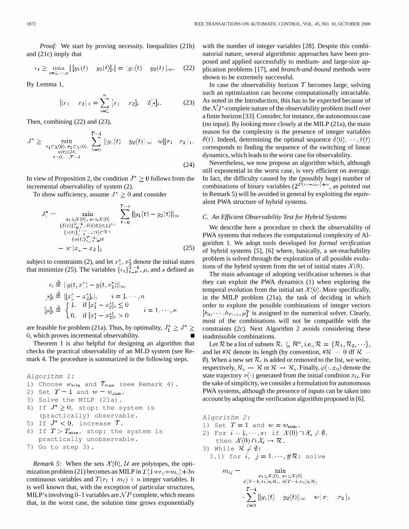
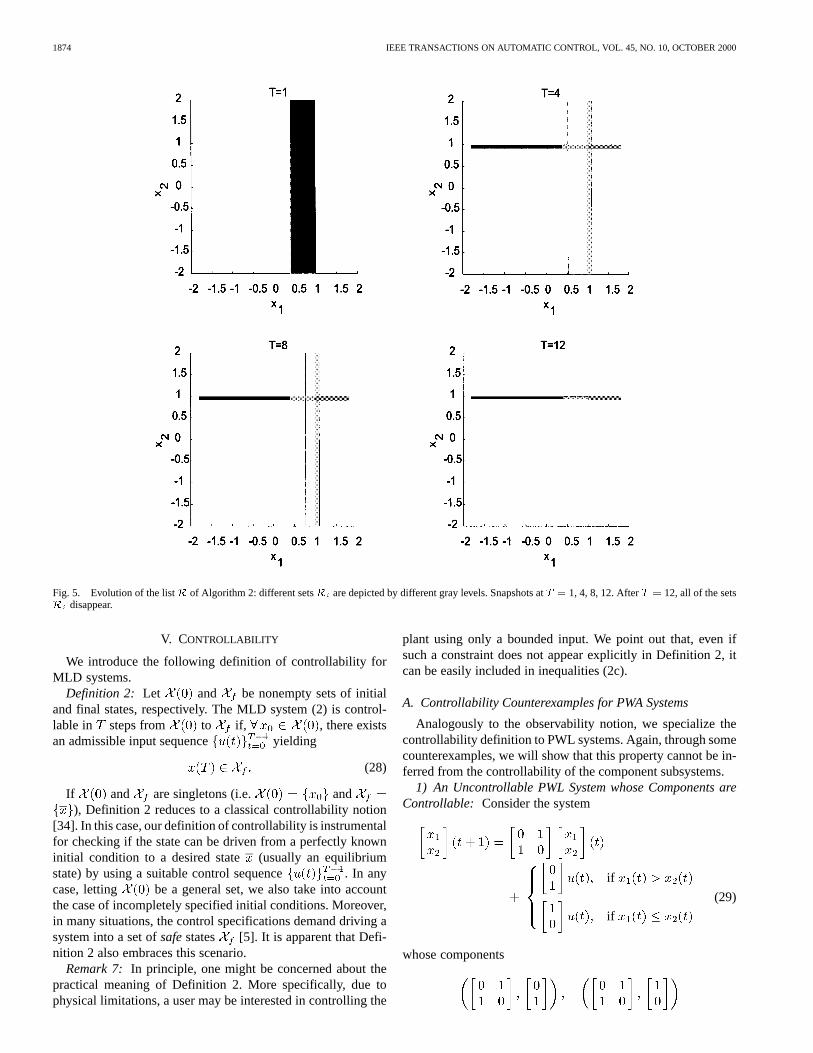
As an illustrative example, we apply Algorthm 2 to system(16) with and . The observ-ability parameters are chosen as and .In Fig. 5, the sets in the list are plotted in different gray levelsat times 1, 4, 8, 12. Note that, due to the evolution of thesystem and the fathoming criterion, the vertical set in the region

progressively shrinks and, for , it disap-pears. Algorthm 2 terminates by finding practical incrementalobservability in 12 steps, in accordance with the analytic resultsof Section IV-A-1 (CPU time: 22.8 s on a Pentium II 300 run-ning Matlab 5.3).

D. A Deadbeat Observer for Hybrid Systems

Proposition 3 provides a deadbeat observer for hybrid sys-tems (2). In a certain sense, it is a counterpart of [30, Theorem2.10].

Proposition 3: Let be the minimizingsequence of the following least squares problem:

subject to

(27)

where , , are the collection ofpast inputs and outputs, and is any time horizon such thatDefinition 1 is satisfied. Then is an estimate of the stateand , , where is the minimumtime horizon for observability.

Proof: After input/output pairs have been collected, theminimum in problem (27) is 0, and the minimizer is

because, otherwise, there would exist astate which is indistinguishable from the true state

based on the observed output sequence.Note that the optimization problem (27) is a mixed-integer

quadratic program, for which efficient solvers exist [16]. AnMILP formulation can be obtained by using 1- or-norms, asin Theorem 1, instead of the squared 2-norm.

As observed in Remark 5, the optimization problem (27) iscomplete, and therefore computationally expensive for

large . Again, the complexity arises from the need for deter-mining the sequence of switches of the linear dynamics whichhas occurred between time and time . Nevertheless,the completeness of the problem of solving (27) does notimply that simpler observers do not exist for hybrid systems.


Fig. 5. Evolution of the listR of Algorithm 2: different setsR are depicted by different gray levels. Snapshots atT = 1, 4, 8, 12. AfterT = 12, all of the setsR disappear.

V. CONTROLLABILITY

We introduce the following definition of controllability forMLD systems.

Definition 2: Let and be nonempty sets of initialand final states, respectively. The MLD system (2) is control-lable in steps from to if, , there existsan admissible input sequence yielding

(28)

If and are singletons (i.e. and), Definition 2 reduces to a classical controllability notion

[34]. In this case, our definition of controllability is instrumentalfor checking if the state can be driven from a perfectly knowninitial condition to a desired state (usually an equilibriumstate) by using a suitable control sequence . In anycase, letting be a general set, we also take into accountthe case of incompletely specified initial conditions. Moreover,in many situations, the control specifications demand driving asystem into a set ofsafestates [5]. It is apparent that Defi-nition 2 also embraces this scenario.

Remark 7: In principle, one might be concerned about thepractical meaning of Definition 2. More specifically, due tophysical limitations, a user may be interested in controlling the

plant using only a bounded input. We point out that, even ifsuch a constraint does not appear explicitly in Definition 2, itcan be easily included in inequalities (2c).

A. Controllability Counterexamples for PWA Systems

Analogously to the observability notion, we specialize thecontrollability definition to PWL systems. Again, through somecounterexamples, we will show that this property cannot be in-ferred from the controllability of the component subsystems.

1) An Uncontrollable PWL System whose Components areControllable: Consider the system

if

if

(29)

whose components


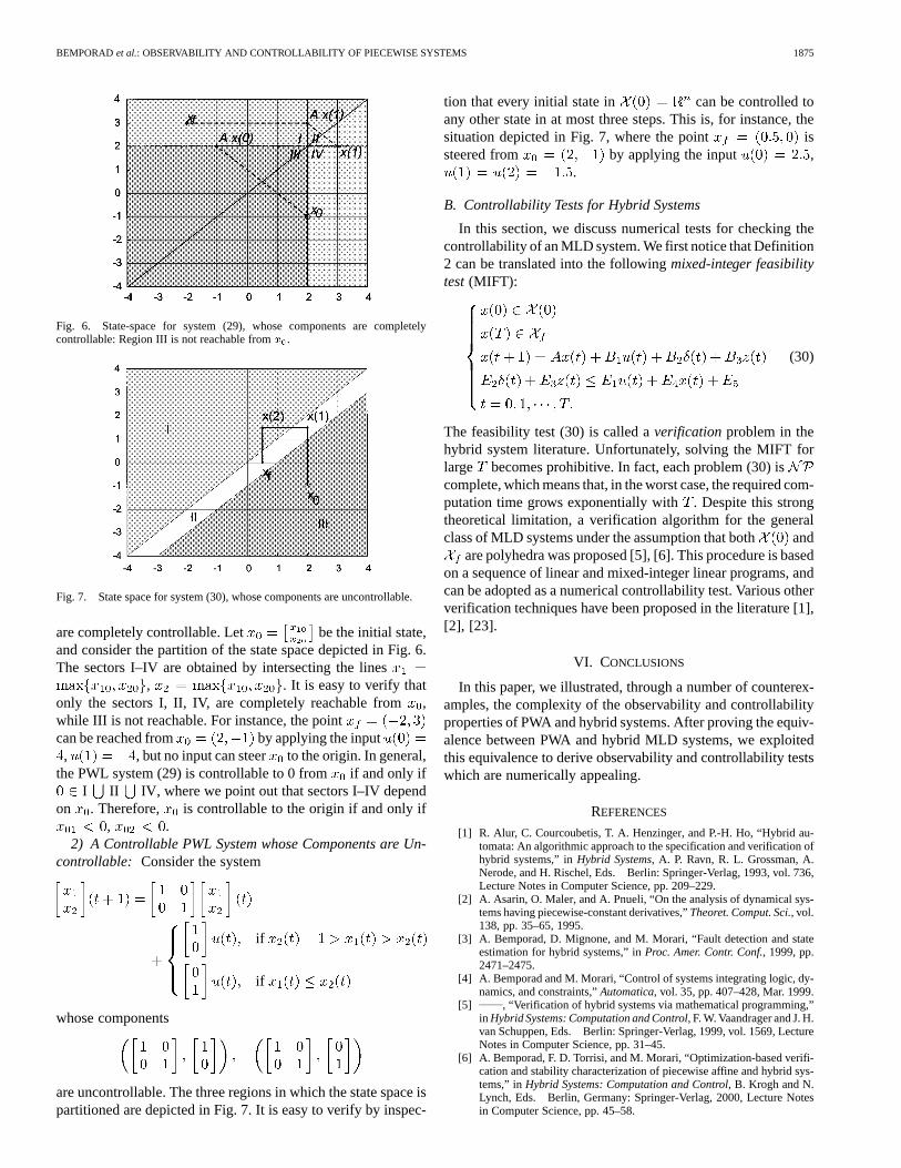
Fig. 6. State-space for system (29), whose components are completelycontrollable: Region III is not reachable fromx .

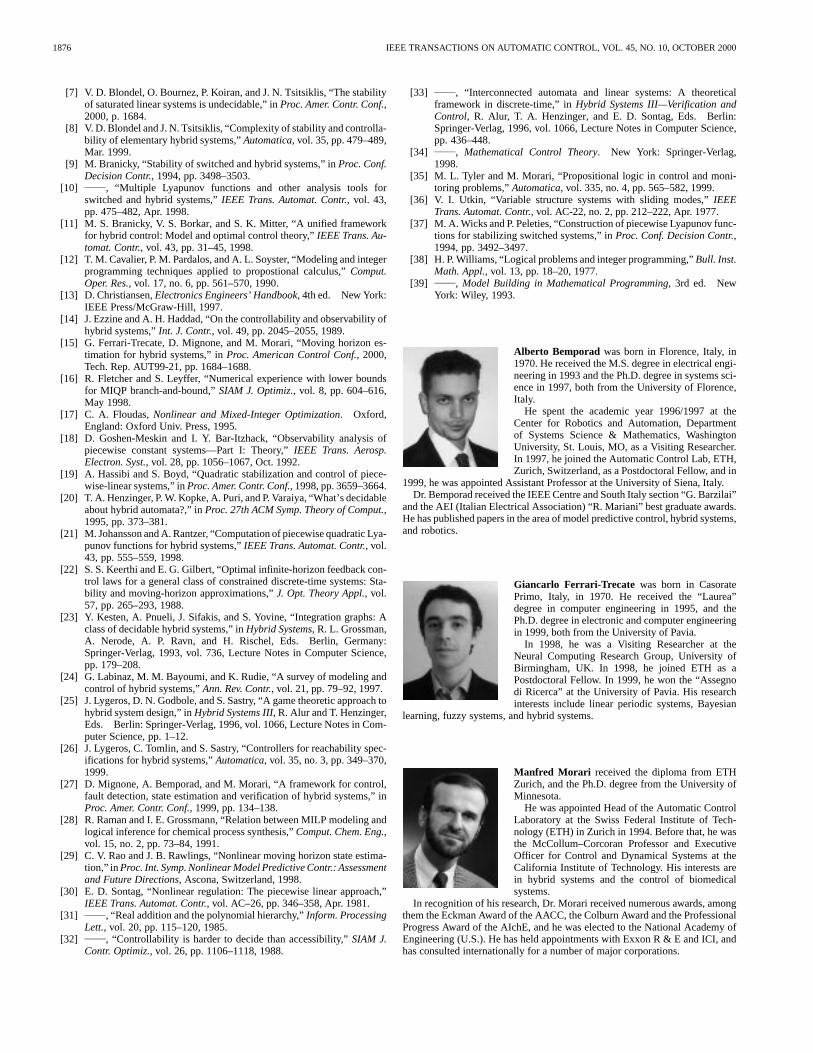
Fig. 7. State space for system (30), whose components are uncontrollable.

are completely controllable. Let be the initial state,and consider the partition of the state space depicted in Fig. 6.The sectors I–IV are obtained by intersecting the lines

, . It is easy to verify thatonly the sectors I, II, IV, are completely reachable from,while III is not reachable. For instance, the pointcan be reached from by applying the input, , but no input can steer to the origin. In general,

the PWL system (29) is controllable to 0 from if and only ifI II IV, where we point out that sectors I–IV depend

on . Therefore, is controllable to the origin if and only if, .

2) A Controllable PWL System whose Components are Un-controllable: Consider the system

if

if

whose components

are uncontrollable. The three regions in which the state space ispartitioned are depicted in Fig. 7. It is easy to verify by inspec-

tion that every initial state in can be controlled toany other state in at most three steps. This is, for instance, thesituation depicted in Fig. 7, where the point issteered from by applying the input ,

.

B. Controllability Tests for Hybrid Systems

In this section, we discuss numerical tests for checking thecontrollability of an MLD system. We first notice that Definition2 can be translated into the followingmixed-integer feasibilitytest(MIFT):

(30)

The feasibility test (30) is called averification problem in thehybrid system literature. Unfortunately, solving the MIFT forlarge becomes prohibitive. In fact, each problem (30) iscomplete, which means that, in the worst case, the required com-putation time grows exponentially with. Despite this strongtheoretical limitation, a verification algorithm for the generalclass of MLD systems under the assumption that both and

are polyhedra was proposed [5], [6]. This procedure is basedon a sequence of linear and mixed-integer linear programs, andcan be adopted as a numerical controllability test. Various otherverification techniques have been proposed in the literature [1],[2], [23].

VI. CONCLUSIONS

In this paper, we illustrated, through a number of counterex-amples, the complexity of the observability and controllabilityproperties of PWA and hybrid systems. After proving the equiv-alence between PWA and hybrid MLD systems, we exploitedthis equivalence to derive observability and controllability testswhich are numerically appealing.

REFERENCES

[1] R. Alur, C. Courcoubetis, T. A. Henzinger, and P.-H. Ho, “Hybrid au-tomata: An algorithmic approach to the specification and verification ofhybrid systems,” inHybrid Systems, A. P. Ravn, R. L. Grossman, A.Nerode, and H. Rischel, Eds. Berlin: Springer-Verlag, 1993, vol. 736,Lecture Notes in Computer Science, pp. 209–229.

[2] A. Asarin, O. Maler, and A. Pnueli, “On the analysis of dynamical sys-tems having piecewise-constant derivatives,”Theoret. Comput. Sci., vol.138, pp. 35–65, 1995.

[3] A. Bemporad, D. Mignone, and M. Morari, “Fault detection and stateestimation for hybrid systems,” inProc. Amer. Contr. Conf., 1999, pp.2471–2475.

[4] A. Bemporad and M. Morari, “Control of systems integrating logic, dy-namics, and constraints,”Automatica, vol. 35, pp. 407–428, Mar. 1999.

[5] , “Verification of hybrid systems via mathematical programming,”in Hybrid Systems: Computation and Control, F. W. Vaandrager and J. H.van Schuppen, Eds. Berlin: Springer-Verlag, 1999, vol. 1569, LectureNotes in Computer Science, pp. 31–45.

[6] A. Bemporad, F. D. Torrisi, and M. Morari, “Optimization-based verifi-cation and stability characterization of piecewise affine and hybrid sys-tems,” inHybrid Systems: Computation and Control, B. Krogh and N.Lynch, Eds. Berlin, Germany: Springer-Verlag, 2000, Lecture Notesin Computer Science, pp. 45–58.


[7] V. D. Blondel, O. Bournez, P. Koiran, and J. N. Tsitsiklis, “The stabilityof saturated linear systems is undecidable,” inProc. Amer. Contr. Conf.,2000, p. 1684.

[8] V. D. Blondel and J. N. Tsitsiklis, “Complexity of stability and controlla-bility of elementary hybrid systems,”Automatica, vol. 35, pp. 479–489,Mar. 1999.

[9] M. Branicky, “Stability of switched and hybrid systems,” inProc. Conf.Decision Contr., 1994, pp. 3498–3503.

[10] , “Multiple Lyapunov functions and other analysis tools forswitched and hybrid systems,”IEEE Trans. Automat. Contr., vol. 43,pp. 475–482, Apr. 1998.

[11] M. S. Branicky, V. S. Borkar, and S. K. Mitter, “A unified frameworkfor hybrid control: Model and optimal control theory,”IEEE Trans. Au-tomat. Contr., vol. 43, pp. 31–45, 1998.

[12] T. M. Cavalier, P. M. Pardalos, and A. L. Soyster, “Modeling and integerprogramming techniques applied to propostional calculus,”Comput.Oper. Res., vol. 17, no. 6, pp. 561–570, 1990.

[13] D. Christiansen,Electronics Engineers’ Handbook, 4th ed. New York:IEEE Press/McGraw-Hill, 1997.

[14] J. Ezzine and A. H. Haddad, “On the controllability and observability ofhybrid systems,”Int. J. Contr., vol. 49, pp. 2045–2055, 1989.

[15] G. Ferrari-Trecate, D. Mignone, and M. Morari, “Moving horizon es-timation for hybrid systems,” inProc. American Control Conf., 2000,Tech. Rep. AUT99-21, pp. 1684–1688.

[16] R. Fletcher and S. Leyffer, “Numerical experience with lower boundsfor MIQP branch-and-bound,”SIAM J. Optimiz., vol. 8, pp. 604–616,May 1998.

[17] C. A. Floudas,Nonlinear and Mixed-Integer Optimization. Oxford,England: Oxford Univ. Press, 1995.

[18] D. Goshen-Meskin and I. Y. Bar-Itzhack, “Observability analysis ofpiecewise constant systems—Part I: Theory,”IEEE Trans. Aerosp.Electron. Syst., vol. 28, pp. 1056–1067, Oct. 1992.

[19] A. Hassibi and S. Boyd, “Quadratic stabilization and control of piece-wise-linear systems,” inProc. Amer. Contr. Conf., 1998, pp. 3659–3664.

[20] T. A. Henzinger, P. W. Kopke, A. Puri, and P. Varaiya, “What’s decidableabout hybrid automata?,” inProc. 27th ACM Symp. Theory of Comput.,1995, pp. 373–381.

[21] M. Johansson and A. Rantzer, “Computation of piecewise quadratic Lya-punov functions for hybrid systems,”IEEE Trans. Automat. Contr., vol.43, pp. 555–559, 1998.

[22] S. S. Keerthi and E. G. Gilbert, “Optimal infinite-horizon feedback con-trol laws for a general class of constrained discrete-time systems: Sta-bility and moving-horizon approximations,”J. Opt. Theory Appl., vol.57, pp. 265–293, 1988.

[23] Y. Kesten, A. Pnueli, J. Sifakis, and S. Yovine, “Integration graphs: Aclass of decidable hybrid systems,” inHybrid Systems, R. L. Grossman,A. Nerode, A. P. Ravn, and H. Rischel, Eds. Berlin, Germany:Springer-Verlag, 1993, vol. 736, Lecture Notes in Computer Science,pp. 179–208.

[24] G. Labinaz, M. M. Bayoumi, and K. Rudie, “A survey of modeling andcontrol of hybrid systems,”Ann. Rev. Contr., vol. 21, pp. 79–92, 1997.

[25] J. Lygeros, D. N. Godbole, and S. Sastry, “A game theoretic approach tohybrid system design,” inHybrid Systems III, R. Alur and T. Henzinger,Eds. Berlin: Springer-Verlag, 1996, vol. 1066, Lecture Notes in Com-puter Science, pp. 1–12.

[26] J. Lygeros, C. Tomlin, and S. Sastry, “Controllers for reachability spec-ifications for hybrid systems,”Automatica, vol. 35, no. 3, pp. 349–370,1999.

[27] D. Mignone, A. Bemporad, and M. Morari, “A framework for control,fault detection, state estimation and verification of hybrid systems,” inProc. Amer. Contr. Conf., 1999, pp. 134–138.

[28] R. Raman and I. E. Grossmann, “Relation between MILP modeling andlogical inference for chemical process synthesis,”Comput. Chem. Eng.,vol. 15, no. 2, pp. 73–84, 1991.

[29] C. V. Rao and J. B. Rawlings, “Nonlinear moving horizon state estima-tion,” in Proc. Int. Symp. Nonlinear Model Predictive Contr.: Assessmentand Future Directions, Ascona, Switzerland, 1998.

[30] E. D. Sontag, “Nonlinear regulation: The piecewise linear approach,”IEEE Trans. Automat. Contr., vol. AC–26, pp. 346–358, Apr. 1981.

[31] , “Real addition and the polynomial hierarchy,”Inform. ProcessingLett., vol. 20, pp. 115–120, 1985.

[32] , “Controllability is harder to decide than accessibility,”SIAM J.Contr. Optimiz., vol. 26, pp. 1106–1118, 1988.

[33] , “Interconnected automata and linear systems: A theoreticalframework in discrete-time,” inHybrid Systems III—Verification andControl, R. Alur, T. A. Henzinger, and E. D. Sontag, Eds. Berlin:Springer-Verlag, 1996, vol. 1066, Lecture Notes in Computer Science,pp. 436–448.

[34] , Mathematical Control Theory. New York: Springer-Verlag,1998.

[35] M. L. Tyler and M. Morari, “Propositional logic in control and moni-toring problems,”Automatica, vol. 335, no. 4, pp. 565–582, 1999.

[36] V. I. Utkin, “Variable structure systems with sliding modes,”IEEETrans. Automat. Contr., vol. AC-22, no. 2, pp. 212–222, Apr. 1977.

[37] M. A. Wicks and P. Peleties, “Construction of piecewise Lyapunov func-tions for stabilizing switched systems,” inProc. Conf. Decision Contr.,1994, pp. 3492–3497.

[38] H. P. Williams, “Logical problems and integer programming,”Bull. Inst.Math. Appl., vol. 13, pp. 18–20, 1977.

[39] , Model Building in Mathematical Programming, 3rd ed. NewYork: Wiley, 1993.

Alberto Bemporad was born in Florence, Italy, in1970. He received the M.S. degree in electrical engi-neering in 1993 and the Ph.D. degree in systems sci-ence in 1997, both from the University of Florence,Italy.

He spent the academic year 1996/1997 at theCenter for Robotics and Automation, Departmentof Systems Science & Mathematics, WashingtonUniversity, St. Louis, MO, as a Visiting Researcher.In 1997, he joined the Automatic Control Lab, ETH,Zurich, Switzerland, as a Postdoctoral Fellow, and in

1999, he was appointed Assistant Professor at the University of Siena, Italy.Dr. Bemporad received the IEEE Centre and South Italy section “G. Barzilai”

and the AEI (Italian Electrical Association) “R. Mariani” best graduate awards.He has published papers in the area of model predictive control, hybrid systems,and robotics.

Giancarlo Ferrari-Trecate was born in CasoratePrimo, Italy, in 1970. He received the “Laurea”degree in computer engineering in 1995, and thePh.D. degree in electronic and computer engineeringin 1999, both from the University of Pavia.

In 1998, he was a Visiting Researcher at theNeural Computing Research Group, University ofBirmingham, UK. In 1998, he joined ETH as aPostdoctoral Fellow. In 1999, he won the “Assegnodi Ricerca” at the University of Pavia. His researchinterests include linear periodic systems, Bayesian

learning, fuzzy systems, and hybrid systems.

Manfred Morari received the diploma from ETHZurich, and the Ph.D. degree from the University ofMinnesota.

He was appointed Head of the Automatic ControlLaboratory at the Swiss Federal Institute of Tech-nology (ETH) in Zurich in 1994. Before that, he wasthe McCollum–Corcoran Professor and ExecutiveOfficer for Control and Dynamical Systems at theCalifornia Institute of Technology. His interests arein hybrid systems and the control of biomedicalsystems.

In recognition of his research, Dr. Morari received numerous awards, amongthem the Eckman Award of the AACC, the Colburn Award and the ProfessionalProgress Award of the AIchE, and he was elected to the National Academy ofEngineering (U.S.). He has held appointments with Exxon R & E and ICI, andhas consulted internationally for a number of major corporations.

Documents

Observability and controllability of piecewise affine …moishi/eece571m/articles/BemporadMorari...1864 IEEE TRANSACTIONS ON AUTOMATIC CONTROL, VOL. 45, NO. 10, OCTOBER 2000 Observability