Observability and Controllability of Nonlinear Networks: The Role of Symmetry

Andrew J. Whalen* and Sean N. Brennan†

Department of Mechanical and Nuclear Engineering, and Center for Neural Engineering,The Pennsylvania State University, University Park, Pennsylvania 16802, USA

Timothy D. Sauer‡

Department of Mathematical Sciences, George Mason University, Fairfax, Virginia 22030, USA

Steven J. Schiff§

Departments of Engineering Science and Mechanics, Neurosurgery and Physics, Center for NeuralEngineering, The Pennsylvania State University, University Park, Pennsylvania 16802, USA

(Received 2 October 2014; published 23 January 2015)

Observability and controllability are essential concepts to the design of predictive observer models andfeedback controllers of networked systems. For example, noncontrollable mathematical models of realsystems have subspaces that influence model behavior, but cannot be controlled by an input. Suchsubspaces can be difficult to determine in complex nonlinear networks. Since almost all of the presenttheory was developed for linear networks without symmetries, here we present a numerical and grouprepresentational framework, to quantify the observability and controllability of nonlinear networks withexplicit symmetries that shows the connection between symmetries and nonlinear measures of observ-ability and controllability. We numerically observe and theoretically predict that not all symmetries havethe same effect on network observation and control. Our analysis shows that the presence of symmetry in anetwork may decrease observability and controllability, although networks containing only rotationalsymmetries remain controllable and observable. These results alter our view of the nature of observabilityand controllability in complex networks, change our understanding of structural controllability, and affectthe design of mathematical models to observe and control such networks.

DOI: 10.1103/PhysRevX.5.011005 Subject Areas: Biological Physics, Complex Systems,Nonlinear Dynamics

I. INTRODUCTION

An observer model of a natural system has many usefulapplications in science and engineering, including under-standing and predicting weather or controlling dynamicsfrom robotics to neuronal systems [1]. A fundamentalquestion that arises when utilizing filters to estimate thefuture states of a system is how to choose a model andmeasurement function that faithfully captures the systemdynamics and can predict future states [2,3]. An observer isa model of a system or process that assimilates data fromthe natural system being modeled [4] and reconstructsunmeasured or inaccessible variables. In linear systems, thekey concept to employ a well-designed observer is

observability, which quantifies whether there is sufficientinformation contained in the measurement to adequatelyreconstruct the full system dynamics [5,6].An important problem when studying networks is how

best to observe and control the entire network when onlylimited observation and control input nodes are available.In classic work, Lin [7] described the topologies of graph-directed linear networks that were structurally controllable.Incorporating Lin’s framework, Liu et al. [8] described anefficient strategy to count the number of control pointsrequired for a complex network, which have an interestingdependence on time constant [9]. Structural observabilityis dual to structural controllability [10]. In Ref. [11], therequirements of structural observability incorporated explicituse of transitive components of directed graphs—fullyconnected subgraphs where paths lead from any node toany other node—to identify the minimal number of sitesrequired to observe from a network.All of these prior works depend critically on the

dynamics being linear and generic, in the sense thatnetwork connections are essentially random. Joly [12]showed that transitive generic networks with nonlinearnodal dynamics are observable from any node.

*awhalen@psu.edu†sbrennan@psu.edu‡tsauer@gmu.edu§sschiff@psu.edu

Published by the American Physical Society under the terms ofthe Creative Commons Attribution 3.0 License. Further distri-bution of this work must maintain attribution to the author(s) andthe published article’s title, journal citation, and DOI.

PHYSICAL REVIEW X 5, 011005 (2015)

2160-3308=15=5(1)=011005(18) 011005-1 Published by the American Physical Society

Nevertheless, symmetries are present in natural networks,as evident from their known structures [13] as well as thepresence of synchrony. Recently, Golubitsky et al. [14]proved the rigid phase conjecture—that the presence ofsynchrony in networks implies the presence of symmetriesand vice versa. In particular, synchrony is an intrinsiccomponent of brain dynamics in normal and pathologicalbrain dynamics [15].Our present work is motivated by the following question:

What role do the symmetries and network couplingstrengths play when reconstructing or controlling networkdynamics? The intuition here is straightforward: considerthree linear systems with identical dynamics [diagonalterms of the system matrix A in _xðtÞ ¼ AxðtÞ]. If thecoupling terms are identical (off-diagonal terms of A), it iseasy to show that the resulting observability of individualstates becomes degenerate as the rows and columns of thesystemmatrix become linearly dependent under elementarymatrix operations. For example, consider the trivial case ofa 3 × 3 system matrix of ones:

_x ¼ Ax ¼

264 1 1 1

1 1 1

1 1 1

375264 x1x2x3

375: ð1Þ

The system is degenerate in the sense that there is only onedynamic, as the rows and columns of A are not indepen-dent. This lack of independent rows and columns of thesystem matrix has direct implications for the controllabilityand observability of the system. For example, in this trivialsystem, the difference between any two of the states isconstrained to a constant x1 − x2 ¼ c; thus, there is noinput coupled to the third state x3 that could control both x1and x2 independently from each other. Taking a singlemeasurement in Eq. (1), y ¼ ½1; 0; 0�x, the system is notobservable; however, taking an additional measurement,

y ¼�1; 0; 00; 1; 0

�x;

the system is fully observable. The details of this compu-tation will be explained in detail in the following section.In fact, for the more general case of linear time-varying

networks, group representation theory [16] has beenutilized to show that linear time-varying networks can benoncontrollable or nonobservable due to the presence ofsymmetry in the network [17]. Brought into context, innetworks with symmetry, Rubin and Meadows [17] defineda coordinate transform that decomposes the network intodecoupled observable (controllable) and unobservable(uncontrollable) subspaces, which can then be determinedby inspection like our previous trivial example. Recently,Pecora et al. [18] utilized this same method to showhow separate subsets of complex networks couldsynchronize and desynchronize according to these same

symmetry-defined subspaces. Interestingly, while Ref. [17]has been a rather obscure work, it is based on Wigner’swork in the 1930s applying group representation theory tothe mechanics of atomic spectra [19]. Thus, just as thestructural symmetry of the Hamiltonian can be used tosimplify the solution to the Schrödinger equation [20], thetopology of the coupling in a network can have a profoundimpact on its observation and control.In this article, we extend the exploration of observability

and controllability to network motifs with explicit non-linearities and symmetries. We further explore the effect ofcoupling strength within such networks, as well as spatialand temporal effects on observability and controllability.Lastly, we demonstrate the utility of the linear analysis ofgroup representation theory as a tool with which to gaininsights into the effects of symmetry in nonlinear networks.Our findings apply to any complex network, includingpower grids, the internet, genomic and metabolic networks,food webs, electronic circuits, social organization, andbrains [8,11,18,21].

II. BACKGROUND

From the theories of differential embeddings [22] andnonlinear reconstruction [23,24] we can create a nonlinearmeasure of observability composed of a measurementfunction and its higher Lie derivatives employing thedifferential embedding map [25]. The differential embed-ding map of an observer provides the information containedin a given measurement function and model, which can bequantified by an index [26–28]. Computed from theJacobian of the differential embedding map, the observ-ability index is a matrix condition number that quantifiesthe perturbation sensitivity (closeness to singularity) of themapping created by the measurement function used toobserve the system. There is a dual theory for control-lability, where the differential embedding map is con-structed from the control input function and its higherLie brackets with respect to the nonlinear model function[29,30]. Singularities in the map cause information aboutthe system to be lost and observability to decrease.Additionally, the presence of symmetries in the system’sdifferential equations makes observation difficult fromvariables around which the invariance of the symmetryis manifested [31,32]. We extend this analysis to networksof ordinary differential equations and investigate the effectsof symmetries on observability and controllability of suchnetworks as a function of connection topology, measure-ment function, and connection strength.

A. Linear observability and controllability

In the early 1960s, Kalman introduced the notions ofstate space decomposition, controllability, and observabil-ity into the theory of linear systems [5]. From this workcomes the classic concept of observability for a linear

WHALEN et al. PHYS. REV. X 5, 011005 (2015)

011005-2

time-invariant dynamic system, which defines a “yes” or“no” answer to the question of whether a state can bereconstructed from a measurement using a rank condi-tion check.A dynamic model for a linear (time-invariant) system can

be represented by

_xðtÞ ¼ AxðtÞ þ BuðtÞ;yðtÞ ¼ CxðtÞ; ð2Þ

where x ∈ Rn represents the state variable, u ∈ Rm is theexternal input to the system, and y ∈ Rp is the output(measurement) function of the state variable. Typically,there are less measurements than states, so p < n. Theintuition for observability comes from asking whether aninitial condition can be determined from a finite period ofmeasuring the system dynamics from one or more sensors.That is, given the system in Eq. (2), with xðtÞ ¼ eAtx0 andBu ¼ 0, determine the initial condition x0 from measure-ment yðtÞ; 0 ≤ t ≤ T. To evaluate this locally, we take thehigher derivatives of yðtÞ:

yðtÞ ¼ CxðtÞ_y ¼ C _xðtÞ ¼ CAxðtÞy ¼ CA _xðtÞ ¼ CA2xðtÞ...

yðn−1Þ ¼ CAn−1xðtÞ: ð3Þ

Factoring the x terms and putting y and its higherderivatives in matrix form, we have a mapping from outputsto states 2

666666664

y

_y

y

..

.

yðn−1Þ

3777777775¼

2666666664

C

CA

CA2

..

.

CAn−1

3777777775x; ð4Þ

where the linear observability matrix [33] is defined as

O≡

266666664

C

CA

CA2

..

.

CAn−1

377777775: ð5Þ

The finite limit of taking derivatives in Eq. (3) comes from theCayley-Hamilton theorem, which specifies that any squarematrixA satisfies its own characteristic equation, which is the

polynomial pðλÞ ¼ 0, where pðλÞ ¼ detðλIn − AÞ. In otherwords, An is spanned by the lower powers of A, from A0 toAn−1,

yðtÞ ¼ CeAtx0; with eAt ≡Xn−1k¼0

αkðtÞAk;

yðtÞ ¼ ½α0ðtÞCþ α1ðtÞCAþ α2ðtÞCA2

þ � � � þ αn−1ðtÞCAn−1�x0: ð6Þ

Thus, if the observability matrix spans n space[rankðOÞ ¼ n], the initial condition x0 can be determined,as the mapping x0 ¼ ðOTOÞ−1OTyðtÞ from output to statesexists and is unique. More formally, the system Eq. (2)is locally observable (distinguishable at a point x0) ifthere exists a neighborhood of x0 such that x0 ≠ x1 ⇒yðx0Þ ≠ yðx1Þ.In a similar fashion, the linear controllability matrix is

derived from asking whether an input uðtÞ can be found totake any initial condition xð0Þ ¼ x0 to arbitrary positionxðTÞ ¼ xf in a finite period of time T. For the sake ofsimplicity, we assume a single input uðtÞ and take thehigher derivatives of _xðtÞ ¼ AxðtÞ þ BuðtÞ up to theðn − 1Þth derivative of uðtÞ (again using the Cayley-Hamilton theorem):

_xðtÞ ¼ AxðtÞ þ BuðtÞxðtÞ ¼ A2xðtÞ þ ABuðtÞ þ B _uðtÞxðtÞ ¼ A3xðtÞ þ A2BuðtÞ þ AB _uðtÞ þ BuðtÞ...

xðnÞðtÞ ¼ AnxðtÞ þ An−1BuðtÞ þ An−2B _uðtÞ þ � � �þ Buðn−1ÞðtÞ; ð7Þ

which gives us a mapping from input to states2666666664

_xðtÞxðtÞ...

xðn−1ÞðtÞxðnÞðtÞ

3777777775−

2666666664

A

A2

..

.

Aðn−1Þ

AðnÞ

3777777775xðtÞ ¼ Q

2666666664

uðtÞ_uðtÞ...

uðn−2ÞðtÞuðn−1ÞðtÞ

3777777775; ð8Þ

where the linear controllability matrix is defined [33] as

Q≡ ½B;AB; A2B � � � ; An−1B �: ð9Þ

B. Differential embeddings and nonlinear observability

From early work on the nonlinear extensions of observ-ability in the 1970s [29,30], it was shown that theobservability matrix for nonlinear systems could beexpressed using the measurement function and its

OBSERVABILITY AND CONTROLLABILITY OF … PHYS. REV. X 5, 011005 (2015)

011005-3

higher-order Lie derivatives with respect to the nonlinearsystem equations. The core idea is to evaluate a mapping ϕfrom the measurements to the states ϕ: Rp → Rn. Inparticular, Hermann and Krener [30] showed that the spaceof the measurement function is embedded in Rn when themapping from measurement to states is everywhere differ-entiable and injective by the Whitney embedding theorem[22,23]. An embedding is a map involving differentialstructure that does not collapse points or tangent directions[24]; thus, a map ϕ is an embedding when the determinantof the map Jacobian detð∂ϕ=∂xj∀x∈RnÞ is nonvanishing andone to one (injective). In a recent series of papers[25,28,31], Letellier et al. computed the nonlinear observ-ability matrices for the well-known Lorenz and Rösslersystems [34,35] and demonstrated that the order of thesingularities present in the observability matrix (and thusthe amount of intersection between the singularities and thephase space trajectories) was related to the decrease inobservability. It is worth noting that the calculation of theobservability matrix and locally evaluating the conditioningof the matrix over a state trajectory is a straightforwardprocess and much more tractable than analytically deter-mining the singularities (and thus their order) of theobservability matrix of a system of arbitrary order. Theformer is limited only by computational capacity and thedifferentiability of the system equations to order n − 1,where n is the order of the system.For a nonlinear system, we replace AxðtÞ in Eq. (2) by a

nonlinear vector field ANLðxðtÞÞ and assume that the smoothscalar measurement function is taken as yðtÞ ¼ CxðtÞ andthe system equations comprise the nonlinear vector fieldfðxðtÞÞ ¼ ANLðxðtÞÞ (note that if there is no external input,then BuðtÞ ¼ 0, which we assume here to simplify thedisplay of equations). (If Bu ≠ 0, then as long as the input isknown the mapping from output to states can be solved, andthe determination of observability still relies on the con-ditioning of the matrixO.) As in the linear case, we evaluatelocally by taking the higher Lie derivatives of yðtÞ, and forcompactness of notation, dependence on t is implied:

L0fðyðxÞÞ ¼ yðxÞ

L1fðyðxÞÞ ¼ ∇yðxÞ · fðxÞ ¼ ∂yðxÞ

∂x · fðxÞ

L2fðyðxÞÞ ¼

∂∂x ½L

1fðyðxÞÞ� · fðxÞ

..

.

LkfðyðxÞÞ ¼

∂∂x ½L

k−1f ðyðxÞÞ� · fðxÞ; ð10Þ

where LfðyðxÞÞ is the Lie derivative of yðxÞ along the vectorfield fðxÞ. More explicitly, we have x ∈ Rn, so as a vectorexample, the first Lie derivative will take the form

L1fðyðxÞÞ ¼

h ∂yðxÞ∂x1 � � � ∂yðxÞ∂xn

i·

26664f1ðxÞ

..

.

fnðxÞ

37775: ð11Þ

With formal definitions of the measurement (output) func-tion Eq. (2) and its higher Lie derivatives Eq. (10), thedifferential embedding map ϕ is defined as the Lie deriv-atives L0

fðyðxÞÞ…Ln−1f ðyðxÞÞ, where the superscripts re-

present the order of the Lie derivative from 0 to n − 1, wheren is the order of the system ANLðxÞ:

ϕ ¼

26666664

L0fðyðxÞÞ

L1fðyðxÞÞ

..

.

Ln−1f ðyðxÞÞ

37777775: ð12Þ

Taking the Jacobian of the map ϕ, we arrive at theobservability matrix

O≡ ∂ϕ∂x ¼

266664

∂L0fðyðxÞÞ∂x1 � � � ∂L0

fðyðxÞÞ∂xn

..

. . .. ..

.

∂Ln−1f ðyðxÞÞ∂x1 � � � ∂Ln−1

f ðyðxÞÞ∂xn

377775; ð13Þ

which reduces to Eq. (5) for linear system representations.The key intuition here is that in the nonlinear case theobservability matrix becomes a function of the states, wherea linear system is always a constant matrix of parameters.

C. Lie brackets and Nonlinear controllability

The nonlinear controllability matrix is developed inRef. [29] from intuitive control problem examples andgiven rigorous treatment in Ref. [30]; in a dual fashion toobservability, the controllability matrix is a mappingconstructed from the input function and its higher-orderLie brackets. The Lie bracket is an algebraic operation ontwo vector fields fðxÞ;gðxÞ ∈ Rn that creates a third vectorfield FðxÞ, which when taken with g as the input controlvector u ∈ Rm defines an embedding in Rn that maps theinput to states [30].For a nonlinear system, we replace AxðtÞ in Eq. (2) by a

nonlinear vector field ANLðxðtÞÞ, take the input function asg ¼ BuðtÞ in system Eq. (2), and create Lie brackets withrespect to the nonlinear vector field fðxðtÞÞ ¼ ANLðxðtÞÞ.The Lie bracket is defined as

WHALEN et al. PHYS. REV. X 5, 011005 (2015)

011005-4

ðad1f ; gÞ ¼ ½f;g� ¼ ∂g∂x f −

∂f∂xg

ðad2f ; gÞ ¼ ½f; ½f;g�� ¼ ∂ðad1f ; gÞ∂x f −

∂f∂x ðad

1f ; gÞ

..

.

ðadkf ; gÞ ¼ ½f; ðadk−1f ;gÞ�; ð14Þ

where ðadkf ; gÞ is the adjoint operator and the superscriptsrepresent the order of the Lie bracket. With formaldefinitions of the input function Eq. (2) and its higherLie brackets Eq. (14) from 1 to n, where n is the order of thesystem matrix ANLðxðtÞÞ, the nonlinear controllabilitymatrix is defined as

Q≡ �g; ðad1f ; gÞ;…; ðadnf ; gÞ

�¼ �

g; ½f;g�; ½f½f;g��;…; ½f; ðadn−1f ;gÞ� �: ð15Þ

D. Observability and controllability indices

In systems with real numbers, calculation of the Kalmanrank condition may not yield an accurate measure of therelative closeness to singularity (conditioning) of theobservability matrix. It was demonstrated in Ref. [26] thatthe calculation of a matrix condition number [36] wouldprovide a more robust determination of the ill conditioninginherent in a given observability matrix, since conditionnumber is independent of scaling and is a continuousfunction of system parameters (and states in the genericnonlinear case). We use the inverted form of the observ-ability index δðxÞ given in Ref. [26] so that 0 ≤ δðxÞ ≤ 1,

δðxÞ ¼ jσmin½OTO�jjσmax½OTO�j ; ð16Þ

where σmin and σmax are the minimum and maximumsingular values of OTO, respectively, and δðxÞ ¼ 1 indi-cates full observability while δðxÞ ¼ 0 indicates no observ-ability [37]. Similarly, the controllability index is justEq. (16) with the substitution of Q for O.

III. OBSERVABILITY AND CONTROLLABILTYOF 3-NODE FITZHUGH-NAGUMO NETWORK

MOTIFS

A. Fitzhugh-Nagumo system dynamics

The Fitzhugh-Nagumo (FN) equations [38,39] comprisea general representation of excitable neuronal membrane.The model is a two-dimensional analog of the well-knownHodgkin-Huxley model [40] of an axonal excitable mem-brane. The nonlinear FN model can exhibit a variety ofdynamical modes, which include active transients, limitcycles, relaxation oscillations with multiple time scales,

and chaos [38,41]. A nonlinear connection function will beused to emulate properties of neuronal synapses.The system dynamics at a node are given by the (local

second-order) state space

_vi ¼ c�vi −

v3i3− wi þ

XfNLðvj; dijÞ þ I

�;

_wi ¼ vi − bwi þ a; ð17Þ

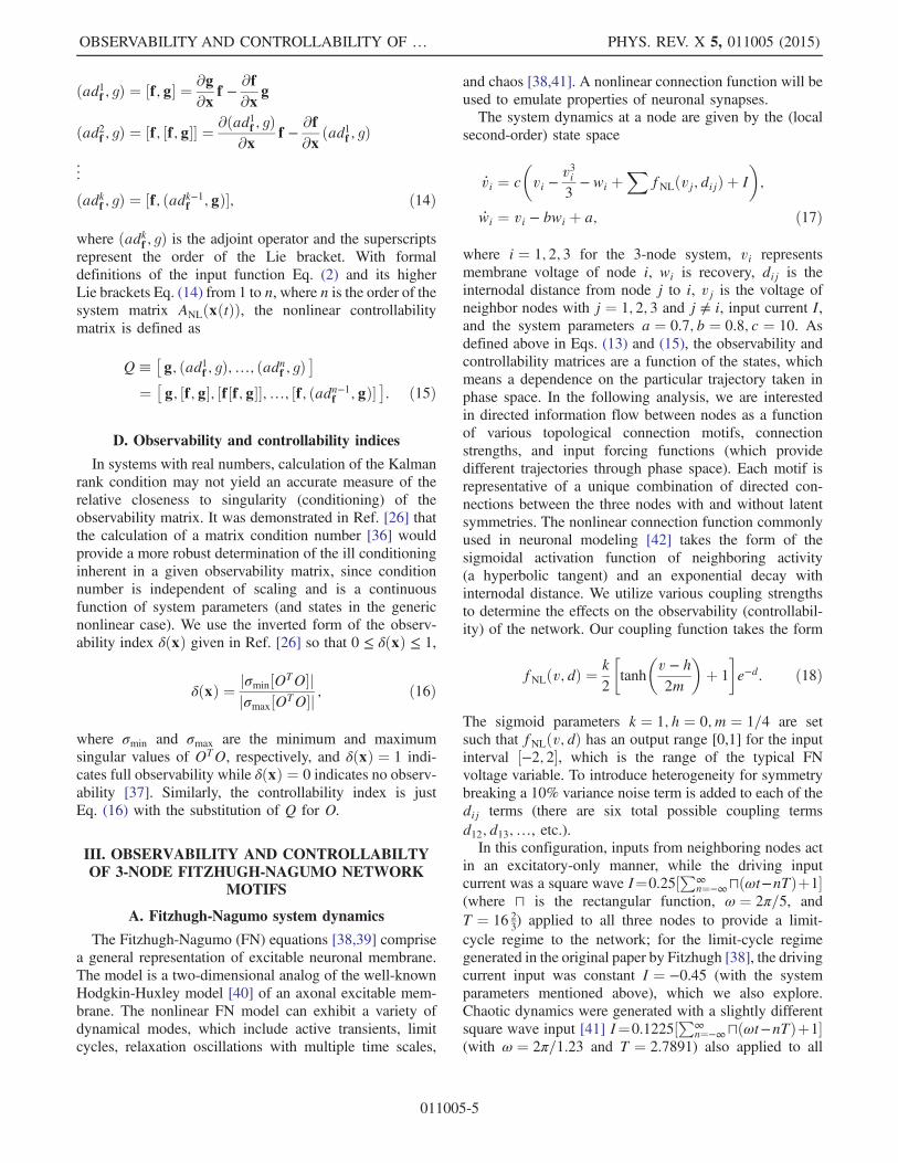
where i ¼ 1; 2; 3 for the 3-node system, vi representsmembrane voltage of node i, wi is recovery, dij is theinternodal distance from node j to i, vj is the voltage ofneighbor nodes with j ¼ 1; 2; 3 and j ≠ i, input current I,and the system parameters a ¼ 0.7; b ¼ 0.8; c ¼ 10. Asdefined above in Eqs. (13) and (15), the observability andcontrollability matrices are a function of the states, whichmeans a dependence on the particular trajectory taken inphase space. In the following analysis, we are interestedin directed information flow between nodes as a functionof various topological connection motifs, connectionstrengths, and input forcing functions (which providedifferent trajectories through phase space). Each motif isrepresentative of a unique combination of directed con-nections between the three nodes with and without latentsymmetries. The nonlinear connection function commonlyused in neuronal modeling [42] takes the form of thesigmoidal activation function of neighboring activity(a hyperbolic tangent) and an exponential decay withinternodal distance. We utilize various coupling strengthsto determine the effects on the observability (controllabil-ity) of the network. Our coupling function takes the form

fNLðv; dÞ ¼k2

�tanh

�v − h2m

�þ 1

�e−d: ð18Þ

The sigmoid parameters k ¼ 1; h ¼ 0; m ¼ 1=4 are setsuch that fNLðv; dÞ has an output range [0,1] for the inputinterval ½−2; 2�, which is the range of the typical FNvoltage variable. To introduce heterogeneity for symmetrybreaking a 10% variance noise term is added to each of thedij terms (there are six total possible coupling termsd12; d13;…, etc.).In this configuration, inputs from neighboring nodes act

in an excitatory-only manner, while the driving inputcurrent was a square wave I¼0.25½P∞

n¼−∞⊓ðωt−nTÞþ1�(where ⊓ is the rectangular function, ω ¼ 2π=5, andT ¼ 16 2

3) applied to all three nodes to provide a limit-

cycle regime to the network; for the limit-cycle regimegenerated in the original paper by Fitzhugh [38], the drivingcurrent input was constant I ¼ −0.45 (with the systemparameters mentioned above), which we also explore.Chaotic dynamics were generated with a slightly differentsquare wave input [41] I¼0.1225½P∞

n¼−∞⊓ðωt−nTÞþ1�(with ω ¼ 2π=1.23 and T ¼ 2.7891) also applied to all

OBSERVABILITY AND CONTROLLABILITY OF … PHYS. REV. X 5, 011005 (2015)

011005-5

three nodes. These various driving input regimes allow awider exploration of the phase space of the system aseach driving input commands a different trajectory, whichwill in turn influence the observability and controllabilitymatrices.

B. Network motifs and simulated data

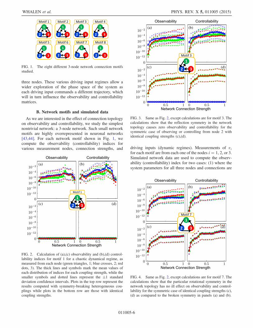
As we are interested in the effect of connection topologyon observability and controllability, we study the simplestnontrivial network: a 3-node network. Such small networkmotifs are highly overrepresented in neuronal networks[43,44]. For each network motif shown in Fig. 1, wecompute the observability (controllability) indices forvarious measurement nodes, connection strengths, and driving inputs (dynamic regimes). Measurements of vi

for each motif are from each one of the nodes i ¼ 1, 2, or 3.Simulated network data are used to compute the observ-ability (controllability) index for two cases: (1) where thesystem parameters for all three nodes and connections are

FIG. 1. The eight different 3-node network connection motifsstudied.

(a) (b)

(c) (d)

FIG. 2. Calculation of (a),(c) observability and (b),(d) control-lability indices for motif 1 for a chaotic dynamical regime, asmeasured from each node (green triangles, 1; blue crosses, 2; reddots, 3). The thick lines and symbols mark the mean values ofeach distribution of indices for each coupling strength, while thesmaller symbols and dotted lines represent the �1 standarddeviation confidence intervals. Plots in the top row represent theresults computed with symmetry-breaking heterogeneous cou-plings while plots in the bottom row are those with identicalcoupling strengths.

(a) (b)

(d)(c)

FIG. 3. Same as Fig. 2, except calculations are for motif 3. Thecalculations show that the reflection symmetry in the networktopology causes zero observability and controllability for thesymmetric case of observing or controlling from node 2 withidentical coupling strengths (c),(d).

(a) (b)

(c) (d)

FIG. 4. Same as Fig. 2, except calculations are for motif 7. Thecalculations show that the particular rotational symmetry in thenetwork topology has no ill effect on observability and control-lability for the symmetric case of identical coupling strengths (c),(d) as compared to the broken symmetry in panels (a) and (b).

WHALEN et al. PHYS. REV. X 5, 011005 (2015)

011005-6

identical, and (2) where the nodes have a heterogeneous(10% variance) symmetry-breaking set of coupling param-eters. To create simulated data, the full six-dimensional FNnetwork equations are integrated from the same initialconditions with the same driving inputs for each node via aRunge-Kutta fourth-order method with time stepΔt ¼ 0.04for 12 000 time steps (with the initial transient discarded) inMATLAB for each test case: (1) limit-cycle and (2) chaoticdynamical regimes, with (a) identical and (b) heterogeneouscoupling (the nodal parameters remain identical through-out). Convergence of solutions is achieved when Δt isdecreased to 0.04. Data are then imported intoMathematica and inserted into symbolic observabilityand controllability matrices (computed for each node),which are then numerically computed to obtain the observ-ability (controllability) indices for each coupling strength.The indices are then averaged over the integration pathsstarting from random initial conditions. These calculationsare summarized in Figs. 2–6 for observability and control-lability, in the chaotic, pulsed limit-cycle, and constantinput limit-cycle dynamical regimes. To facilitate othersreplicating our work, we have archived extensive codein MATLAB and Mathematica in the SupplementalMaterial [45].

IV. RESULTS

A. Motifs with symmetry

For motif 1, the data show that a system with full S3symmetry (due to the connection topology and identicalnodal and coupling parameters) generates zero observabil-ity (controllability) over the entire range of couplingstrengths [Figs. 2(c) and 2(d)]. Similarly, no observability(controllability) is seen from node 2 in motif 3, which has areflection S2 symmetry across the plane through node 2[Figs. 3(c) and 3(d)]. Interestingly, the cyclic symmetry ofmotif 7 does not cause loss of observability (controllability)as shown in Fig. 4; motif 7 has rotational C3 symmetry andvalance 1 connectivity (1 input, 1 output). In motifs 1 and 3the effect of the symmetry is partially broken by introduc-ing a variation in the coupling terms, and the results shownonzero observability (controllability) indices in the plotsfor such heterogeneous coupling [plots (a) and (b) in Figs. 2and 3] with a dependence on the coupling strength.Of particular interest is the substantial loss of observ-

ability (controllability) as the coupling strengths increase tocritical levels for systems containing latent structuralsymmetries in the presence of heterogeneity [motifs 1and 3, plots (a) and (b) in Figs. 2 and 3]. That is, increasingthe coupling strengths when recording (stimulating) from

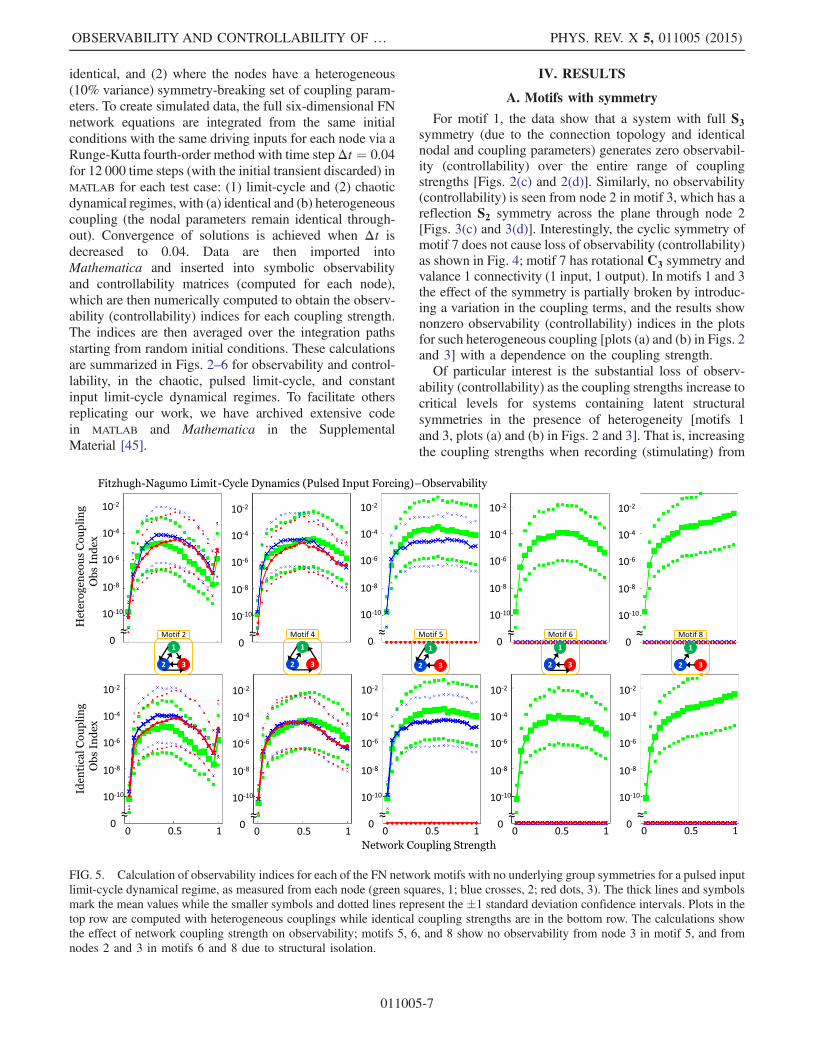
FIG. 5. Calculation of observability indices for each of the FN network motifs with no underlying group symmetries for a pulsed inputlimit-cycle dynamical regime, as measured from each node (green squares, 1; blue crosses, 2; red dots, 3). The thick lines and symbolsmark the mean values while the smaller symbols and dotted lines represent the �1 standard deviation confidence intervals. Plots in thetop row are computed with heterogeneous couplings while identical coupling strengths are in the bottom row. The calculations showthe effect of network coupling strength on observability; motifs 5, 6, and 8 show no observability from node 3 in motif 5, and fromnodes 2 and 3 in motifs 6 and 8 due to structural isolation.

OBSERVABILITY AND CONTROLLABILITY OF … PHYS. REV. X 5, 011005 (2015)

011005-7

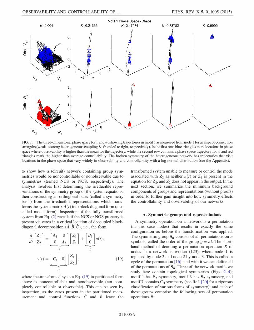
any node in motif 1 or node 2 in motif 3 degradesobservability (controllability) as coupling strengthincreases. A study of the 3D phase plots of the FN voltagevariable in motif 1 (as a function of coupling strength forchaotic dynamics) reveals a blowout bifurcation [46] atlower values of coupling strengths (Fig. 7), and at higherlevels, generalized synchrony [47] and increased observ-ability (controllability), and finally the subsequent decreasein observability (controllability) at the highest levels ofcoupling strength [motif 1 as observed (controlled) fromany node in Fig. 2]. This is demonstrated in motif 1 (Fig. 7),where a bifurcation in the dynamics causes the wanderingtrajectories at weak coupling strengths to collapse onto thelimit-cycle attractor at stronger coupling strengths, and atthe strongest coupling the dynamics reveal a reverse Hopfbifurcation from the limit cycle back into a stableequilibrium.Although motif 7 contains symmetry, the observability

and controllability measures appear unaffected by thepresence of this symmetry; further insight into why thishappens in such networks requires group representationtheory and is presented in Sec. V.

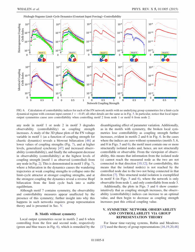
B. Motifs without symmetry

Local output symmetries occur in motifs 2 and 6 whencontrolling from the first and second node, respectively(green and blue traces in Fig. 6), which is remedied by the

disambiguating effect of parameter variation. Additionally,as in the motifs with symmetry, the broken local sym-metries lose controllability as coupling strength furtherincreases, evident in motifs 2 and 6 in Fig. 6. In the caseswhere the indices are zero without symmetries (motifs 5, 6,and 8 in Figs. 5 and 6), the motif must contain one or morestructurally isolated nodes and, hence, are not structurallycontrollable or observable. From the viewpoint of observ-ability, this means that information from the isolated node(s) cannot reach the measured node as the two are notconnected in that direction [10,12]; for controllability, thismeans that the isolated node(s) is not reached by thecontrolled node due to the two not being connected in thatdirection [7]. This structural nodal isolation is exemplifiedin motif 8 (in Figs. 5 and 6), where the network is onlyobservable from node 1, and only controllable from node 3.Additionally, the plots in Figs. 5 and 6 show counter-

intuitively that as coupling strength increases, the observ-ability (controllability) indices can increase to an optimalvalue, and then begin to decrease as coupling strengthincreases past this critical coupling value.

V. SYMMETRIC NETWORK OBSERVABILITYAND CONTROLLABILITY VIA GROUP

REPRESENTATION THEORY

For linear time-varying systems, Rubin and Meadows[17] used the theory of group representations [16,19,20,48]

FIG. 6. Calculation of controllability indices for each of the FN network motifs with no underlying group symmetries for a limit-cycledynamical regime with constant input current I ¼ −0.45; all other details are the same as in Fig. 5. In particular, notice that local input-output symmetries cause zero controllability when controlling motif 2 from node 1 or motif 6 from node 2.

WHALEN et al. PHYS. REV. X 5, 011005 (2015)

011005-8

to show how a (circuit) network containing group sym-metries would be noncontrollable or nonobservable due tosymmetries (termed NCS or NOS, respectively). Theanalysis involves first determining the irreducible repre-sentations of the symmetry group of the system equations,then constructing an orthogonal basis (called a symmetrybasis) from the irreducible representations which trans-forms the systemmatrix AðtÞ into block diagonal form (alsocalled modal form). Inspection of the fully transformedsystem from Eq. (2) reveals if the NCS or NOS property ispresent via zeros in a critical location of decoupled block-diagonal decomposition ðA; B; CÞ, i.e., the form

ddt

�Z1

Z2

�¼

�A1 0

0 A2

�|fflfflfflfflfflfflffl{zfflfflfflfflfflfflffl}

A

�Z1

Z2

�þ�B1

0

�|fflffl{zfflffl}

B

uðtÞ;

yðtÞ ¼�C1 0

�|fflfflfflfflfflffl{zfflfflfflfflfflffl}

C

�Z1

Z2

�; ð19Þ

where the transformed system Eq. (19) in partitioned formabove is noncontrollable and nonobservable (not com-pletely controllable or observable). This can be seen byinspection, as the zeros present in the partitioned meas-urement and control functions C and B leave the

transformed system unable to measure or control the modeassociated with Z2 as neither uðtÞ or Z1 is present in theequation for Z2, and Z2 does not appear in the output. In thenext section, we summarize the minimum backgroundcomponents of groups and representations (without proofs)in order to further gain insight into how symmetry effectsthe controllability and observability of our networks.

A. Symmetric groups and representations

A symmetry operation on a network is a permutation(in this case nodes) that results in exactly the sameconfiguration as before the transformation was applied.The symmetric group Sn consists of all permutations on nsymbols, called the order of the group g ¼ n!. The short-hand method of denoting a permutation operation R ofnodes in a network is written (123), where node 1 isreplaced by node 2 and node 2 by node 3. This is called acycle of the permutation [16], and with it we can define allof the permutations of Sn. Three of the network motifs westudy here contain topological symmetries (Figs. 2–4);motif 1 has S3 symmetry, motif 3 has S2 symmetry, andmotif 7 contains C3 symmetry (see Ref. [20] for a rigorousclassification of various forms of symmetry), and each ofthese groups comprise the following sets of permutationoperations R:

FIG. 7. The three-dimensional phase space for v andw, showing trajectories inmotif 1 asmeasured fromnode 1 for a range of connectionstrengths (weak to strong heterogeneous couplingK, from left to right, respectively). In the first row, blue triangles mark locations in phasespace where observability is higher than the mean for the trajectory, while the second row contains a phase space trajectory for w and redtriangles mark the higher than average controllability. The broken symmetry of the heterogeneous network has trajectories that visitlocations in the phase space that vary widely in observability and controllability with a log-normal distribution (see the Appendix).

OBSERVABILITY AND CONTROLLABILITY OF … PHYS. REV. X 5, 011005 (2015)

011005-9

R∶ S3 ¼ fE; σ1; σ2; σ3; C3; C23g

¼ fE ¼ ð1Þð2Þð3Þσ1 ¼ ð23Þ; σ2 ¼ ð13Þ; σ3 ¼ ð12ÞC3 ¼ ð132Þ; C2

3 ¼ ð123Þg; ð20Þ

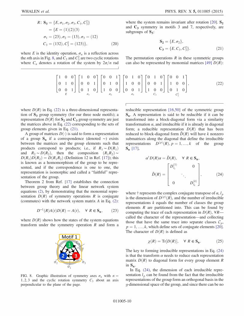
where E is the identity operation, σn is a reflection acrossthe nth axis in Fig. 8, andC3 andC2

3 are two cyclic rotationswhere Cn denotes a rotation of the system by 2π=n rad

where the system remains invariant after rotation [20]. S2and C3 symmetry in motifs 3 and 7, respectively, aresubgroups of S3:

S2 ¼ fE; σ2g;C3 ¼ fE;C3; C2

3g: ð21Þ

The permutation operations R in these symmetric groupscan also be represented by monomial matrices [49] DðRÞ:

264 1 0 0

0 1 0

0 0 1

375

E

264 1 0 0

0 0 1

0 1 0

375

σ1

264 0 0 1

0 1 0

1 0 0

375

σ2

264 0 1 0

1 0 0

0 0 1

375

σ3

264 0 1 0

0 0 1

1 0 0

375

C3

264 0 0 1

1 0 0

0 1 0

375

C23

; ð22Þ

where DðRÞ in Eq. (22) is a three-dimensional representa-tion of S3 group symmetry (for our three node motifs); arepresentationDðRÞ for S2 andC3 group symmetry are justthe matrices above in Eq. (22) corresponding to the sets ofgroup elements given in Eq. (21).A group of matrices Dð·Þ is said to form a representation

of a group Sn if a correspondence (denoted ∼) existsbetween the matrices and the group elements such thatproducts correspond to products; i.e., if R1 ∼DðR1Þand R2 ∼DðR2Þ, then the composition ðR1R2Þ ∼DðR1ÞDðR2Þ ¼ DðR1R2Þ (Definition 12 in Ref. [17]); thisis known as a homomorphism of the group to be repre-sented, and if the correspondence is one to one, therepresentation is isomorphic and called a “faithful” repre-sentation of the group.Theorem 2 from Ref. [17] establishes the connection

between group theory and the linear network systemequations (2), by demonstrating that the monomial repre-sentation DðRÞ of symmetry operations R is conjugate(commutes) with the network system matrix A in Eq. (2):

D−1ðRÞAðtÞDðRÞ ¼ AðtÞ; ∀ R ∈ Sn; ð23Þ

where DðRÞ shows how the states of the system equationstransform under the symmetry operation R and form a

reducible representation [16,50] of the symmetric groupSn. A representation is said to be reducible if it can betransformed into a block-diagonal form via a similaritytransformation α, and irreducible if it is already in diagonalform; a reducible representation DðRÞ that has beenreduced to block-diagonal form DðRÞ will have k nonzerosubmatrices along the diagonal that define the irreduciblerepresentations DðpÞðRÞ; p ¼ 1;…; k of the groupSn [17],

α†DðRÞα ¼ DðRÞ; ∀ R ∈ Sn;

DðRÞ ¼

26664Dð1Þ

l10

. ..

0 DðkÞlk

37775; ð24Þ

where † represents the complex conjugate transpose of α, lpis the dimension of DðpÞðRÞ, and the number of irreduciblerepresentations k equals the number of classes the groupelements R are partitioned into. This can be found bycomputing the trace of each representation in DðRÞ, ∀R—called the character of the representation—and collectingthose that have the same trace into separate classes Cp,p ¼ 1;… ; k, which define sets of conjugate elements [20].The character of DðRÞ is defined as

χðRÞ ¼ Tr½DðRÞ�; ∀ R ∈ Sn: ð25Þ

The key to forming irreducible representations in Eq. (24)is that the transform α needs to reduce each representationmatrix DðRÞ to diagonal form for every group element Rin Sn.In Eq. (24), the dimension of each irreducible repre-

sentation lp can be found from the fact that the irreduciblerepresentations of the group form an orthogonal basis in theg-dimensional space of the group, and since there can be no

FIG. 8. Graphic illustration of symmetry axes σn with n ¼1; 2; 3 and the cyclic rotation symmetry C3 about an axisperpendicular to the plane of the page.

WHALEN et al. PHYS. REV. X 5, 011005 (2015)

011005-10

more than g independent vectors in the orthogonal basis, itcan be shown [48] that

Xkp¼1

l2p ¼ g; ð26Þ

where the sum is over the number of irreducible repre-sentations (or classes of conjugate group elements) k. Someof the irreducible representations DðpÞðRÞ will appear inDðRÞ more than once while others may not appear at all;the character of the representation completely determinesthis, and the number of times ap that DðpÞðRÞ appears inDðRÞ is defined in Ref. [20] as

ap ¼ 1

g

XR

χðpÞðRÞ�χðRÞ; ð27Þ

where χðpÞðRÞ is the trace of DðpÞðRÞ, the asterisk denotescomplex conjugate, and χðRÞ is the trace of DðRÞ.

B. Construction of the similarity transform α

We examine motif 3 in Fig. 3, which has S2 symmetry[51]. Determined from Eq. (25), there are two classes ofgroup elements C1 ¼ fEg and C2 ¼ fσ2g, and reduction ofDðRÞ yields the two, one-dimensional [l1 ¼ l2 ¼ 1 com-puted from Eq. (26)] irreducible representations Dð1ÞðRÞand Dð2ÞðRÞ of S2:

R E σ2

Dð1ÞðRÞ 1 1

Dð2ÞðRÞ 1 −1; ð28Þ

where each entry in DðpÞ corresponds to the elements ofDðRÞ above in Eq. (22), where R ¼ fE; σ2g as in Eq. (21),and from Eq. (27), Dð1ÞðRÞ appears two times whileDð2ÞðRÞ appears once in DðRÞ.A procedure for transforming the reducible representa-

tion DðRÞ of a symmetry group Sn to block-diagonal formis presented in Refs. [17,50]. A unitary transformation α isconstructed from the normalized linearly independent

columns of the n × n generating matrix GðpÞi ,

GðpÞi ¼

XR

DðpÞðRÞ�iiDðRÞ; ð29Þ

where DðpÞðRÞii is the ði; iÞth diagonal entry of an lp-dimensional irreducible representation p (hence,i ¼ 1;…; lp) of the symmetry group Sn and the asterisk

denotes complex conjugate. Each matrix GðpÞi will con-

tribute ap linearly independent columns from Eq. (27) toform the coordinate transformation matrix α. UsingEqs. (28) and (29) and iterating through all lp rows ofeach of the k irreducible representations in Eq. (24), weconstruct α for motif 3:

Gð1Þ1 ¼

XR∈S2

Dð1ÞðRÞ�11DðRÞ

¼ 1

264 1 0 0

0 1 0

0 0 1

375þ 1

264 0 0 1

0 1 0

1 0 0

375 ¼

264 1 0 1

0 2 0

1 0 1

375;ð30Þ

where each linearly independent column of G is a columnof α. After normalizing, we have

264 1

0

1

375;

264 0

2

0

375!

normalize

2664

1ffiffi2

p

0

1ffiffi2

p

3775;

264 0

1

0

375 ¼

264 α11 α21

α12 α22

α13 α23

375;

ð31Þ

which defines the first and second columns of α.Continuing, we have

Gð2Þ1 ¼

XR∈S2

Dð2ÞðRÞ�11DðRÞ

¼ 1

264 1 0 0

0 1 0

0 0 1

375 − 1

264 0 0 1

0 1 0

1 0 0

375 ¼

264 1 0 −1

0 0 0

−1 0 1

375;

ð32Þ

which yields the final column of α (after normalization):

264 1

0

−1

375!

normalize

264

1ffiffi2

p

0

− 1ffiffi2

p

375 ¼

264 α31

α32

α33

375: ð33Þ

Now, the coordinate transformation matrix α is

α ¼

2664

1ffiffi2

p 0 1ffiffi2

p

0 1 0

1ffiffi2

p 0 − 1ffiffi2

p

3775: ð34Þ

Motif 3 in Fig. 3 has connection matrix A3:

A3 ¼

264 0 1 0

1 0 1

0 1 0

375: ð35Þ

To control from nodes 1, 2, and 3, respectively, the Bmatrixtakes the form

OBSERVABILITY AND CONTROLLABILITY OF … PHYS. REV. X 5, 011005 (2015)

011005-11

B1;2;3 ¼

264 1

0

0

375;

264 0

1

0

375;

264 0

0

1

375; ð36Þ

and to observe from nodes 1, 2, and 3, respectively, theC matrix takes the form

C1;2;3 ¼ ½ 1 0 0 �; ½ 0 1 0 �; ½ 0 0 1 �: ð37Þ

The block-diagonalized system ðA3; B; CÞ is formed withthe substitution Z ¼ α†x, and (A3; B; C) in Eqs. (35)–(37)becomes

A3∶ α†A3α ¼

264 0

ffiffiffi2

p0ffiffiffi

2p

0 0

0 0 0

375;

B∶ α†B1;2;3 ¼

2664

1ffiffi2

p

01ffiffi2

p

3775;

264 0

1

0

375;

2664

1ffiffi2

p

0−1ffiffi2

p

3775;

C∶ C1;2;3α ¼h

1ffiffi2

p 0 1ffiffi2

pi; ½ 0 1 0 �;

h1ffiffi2

p 0 −1ffiffi2

pi.

ð38Þ

By inspection of the transformed system Eq. (38), itbecomes clear that motif 3 is noncontrollable and non-observable from node 2 due to symmetry alone (NCS andNOS); i.e. the transformed system in modal coordinates,

ddt

264Z1

Z2

Z3

375 ¼

264 0

ffiffiffi2

p0ffiffiffi

2p

0 0

0 0 0

375264Z1

Z2

Z3

375þ

264 0

1

0

375uðtÞ;

yðtÞ ¼ ½ 0 1 0 �

264Z1

Z2

Z3

375; ð39Þ

is NCS and NOS as the mode associated with Z3 cannot bereached by the input B2 nor can its measurement be inferredfrom the output C2 as in Eq. (19).The procedure to reduce motif 1 is accomplished in a

similar fashion (full computation of α is detailed in theAppendix) and the connection matrix A1 and its reducedform A1 is

A1 ¼

264 0 1 1

1 0 1

1 1 0

375; A1 ¼

264 2 0 0

0 −1 0

0 0 −1

375; ð40Þ

while the transformed B and C matrices in Eqs. (36) and(37) are

B1;2;3 ¼

2664

1ffiffi3

p ffiffi23

q0

3775;

2664

1ffiffi3

p

−1ffiffi6

p

1ffiffi2

p

3775;

2664

1ffiffi3

p

−1ffiffi6

p

−1ffiffi2

p

3775; C123 ¼ BT

1;2;3: ð41Þ

At first glance, it appears that motif 1 is NCS and NOS formeasurement and control from node 1 only, and fullycontrollable and observable from node 2 and 3; however,there is a subtle nuance to the controllability and observ-ability of the diagonal form used in Ref. [17] andconsolidated in Eq. (19) to show noncontrollability andnonobservability by inspection.It is well known that every nonsingular n × n matrix has

n eigenvalues λn, and that a matrix with repeated eigen-values of algebraic multiplicity mi will have a degeneracy1 ≤ qi ≤ mi associated with the number of linearly inde-pendent eigenvectors for repeated eigenvalue λi. Thisdegeneracy qi is also called the geometric multiplicity ofλi, and is equal to the dimension of the null space of A − Iλi[52]. When utilizing similarity transforms to reduce amatrix to diagonal (modal) form, this degeneracy in theeigenvectors (brought about by repeated eigenvalues)results in a transformed matrix that is almost diagonal,called the Jordan form matrix. The Jordan form is com-posed of submatrices of dimension mi—called Jordanblocks—that have ones on the superdiagonal of eachJordan block Ji associated with the generalized eigenvec-tors of a repeated eigenvalue λi. The diagonal form inEq. (19) is a special case of a Jordan form where thematrices on the diagonal are Jordan blocks of dimensionone. This is known as the fully degenerate case withqi ¼ mi, and the Jordan form will have mi separate 1×1Jordan blocks associated with each eigenvalue λi.The observability and controllability of systems in

Jordan form hinges on where the zeros appear in thepartitioned Ci and Bi matrices, where subscript i indicates apartition associated with a particular Jordan block Ji. Givenin Refs. [52,53], the conditions for controllability andobservability of a system in Jordan form are: 1. The firstcolumns of Ci or the last rows of Bi must form a linearlyindependent set of vectors fc11…c1qig or fb1e…bqieg(subscript e indicates the last row) corresponding to theqi Jordan blocks Jλi1 � � � Jλiqi for repeated eigenvalue λi.2. c1p ≠ 0 or bpe ≠ 0 when there is only one Jordan block

Jλip associated with eigenvalue λi. 3. For single output andsingle input systems, the partitions of Ci and Bi arescalars—which are never linearly independent—thus, eachrepeated eigenvalue must have only one Jordan block Jλiiassociated with it for observability or controllability,respectively. From these criteria, we can now see thatthe transformed system for motif 1 in Eq. (40) containsthree 1 × 1 Jordan blocks, two of which are associated withthe repeated eigenvalue λ2 ¼ −1, which violates condition(3); thus, we conclude it is NCS and NOS.

WHALEN et al. PHYS. REV. X 5, 011005 (2015)

011005-12

C. Motif 7 and networks containingonly rotation groups

In Ref. [17], it was shown how the rth component of αvanishes according to the matrices DðpÞðRr

rÞ, where Rrr

represents a subgroup of the group operations (R) thattransform the rth state variable into itself. Subsequently,two theorems were proven that make use of this fact tosimplify the analysis of networks that have a single input oroutput coupled only to the rth state variable, which isprecisely parallel to our analysis in Sec. IV. A paraphrasingof Theorems 6 and 12 from Ref. [17] for controllability andobservability states that such a single input or outputnetwork is NCS or NOS if and only if there is an irreduciblerepresentation DðpÞðRÞ that appears in DðRÞ andX

Rrr

srrDðpÞðRrrÞ�ii ¼ 0 ð42Þ

for some value of i, where srr is þ1 or −1 as Rrr transforms

state variable xr into itself with a plus or minus sign [in ourmotifs, DðRÞ is a permutation representation; thus,srr ¼ þ1]. For this theorem to hold, the equality inEq. (42) must be checked for all possible p for DðpÞðRÞthat appear in DðRÞ via Eq. (27).Applying Eq. (42) to motif 7, the irreducible represen-

tations for C3 symmetry are

R E C3 C23

Dð1ÞðRÞ 1 1 1

Dð2ÞðRÞ 1 ω ω2

Dð3ÞðRÞ 1 ω2 ω

; ð43Þ

where ω ¼ e2πi=3. From the subset Eq. (21) of Eq. (22), wefind that the only operation Rr

r that leaves either node 1, 2,or 3 (state variables x1, x2, or x3) invariant is just theidentity operation E, and it is straightforward to see thatEq. (42) is not equal to 0 for all choices of p, i, and r sincethere is only one group operation that leaves the rth statevariable invariant, Rr

r ¼ E, for r ¼ 1; 2; 3. Thus, motif 7cannot be NCS or NOS and must be controllable andobservable from any node. Corollary 1 to Theorem 6 fromRef. [17] contains and expands this result directly to anynetwork with only rotational symmetry (i.e., Cn groups),with the caveat that a network with a state variable that isinvariant under all the group operations (motif 7 does nothave such a state variable) will be NCS and NOS if theinput and output are coupled to that variable.These representation group theoretic results explain our

nonlinear results in Sec. IV, and clearly demonstrate thatdifferent types of symmetry have different effects on thecontrollability and observability of the networks containingthem. While we explicitly assume system matrices withzeros on the diagonal (for simplicity of the calculations),these results hold with generic entries on the diagonal as

long as those entries are chosen to preserve the symmetry(e.g., the system matrix A for motif 1 and 7 has a11 ¼a22 ¼ a33 and motif 3 has a11 ¼ a33, not shown).Linearization of the system equations in Eq. (17) wouldresult in a system matrix A with a nonzero diagonal [9], andis typically done in the analysis of nonlinear networks [18]when utilizing such linear analysis techniques. Our com-putational results demonstrate the utility of this approach inproviding insight into the controllability and observabilityof complex nonlinear networks that have not beenlinearized.

D. Application to structural controllabilityand observability

It is interesting to note that the demonstration of ourresults above and those in Ref. [17] complement andexpand Lin’s seminal theorems on structural controllability[7]. Essentially, a network with system matrix A and inputfunction B [the pair ðA; BÞ] are assumed to have two typesof entries, nonzero generic entries and fixed entries whichare zero. The position of the zero entries leads to the notionof the structure of the system, where different systems withzeros in the same locations are considered structurallyequivalent. With this definition of structure, we arrive at thedefinition for structural controllability, which states that apair ðA0; B0Þ is structurally controllable if and only if thereexists a controllable pair ðA00; B00Þwith the same structure asðA0; B0Þ. The major assumption of this work is that a systemdeemed to be structurally controllable could indeed beuncontrollable due to the specific entries in A and B, whichfor a practical application are assumed to be uncertainestimates of the system parameters and thus subject tomodification. While Lin’s theorems did not explicitly coversymmetry, any network pair ðA;BÞ containing symmetry

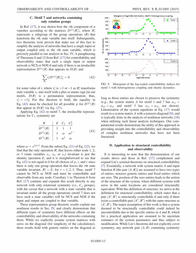
FIG. 9. Histogram of the log-scaled controllability indices formotif 1 with heterogeneous coupling and chaotic dynamics.

OBSERVABILITY AND CONTROLLABILITY OF … PHYS. REV. X 5, 011005 (2015)

011005-13

implies constraints on the nonzero entries in ðA; BÞ, whichis necessary to guarantee that symmetry is present. Thus,considering only Ref. [7], a network with symmetry couldbe structurally controllable (observable [10]) as long asthe graph of the system contains no dilations (defined in theAppendix) or isolated nodes, but NCS (NOS) due to thesymmetry. These two theorems together paint a morecomplete picture of controllability (observability) thaneither alone, as shown in Secs. IV and V, where both areused in concert to explain and understand why certainnetwork motifs are not controllable or observable fromparticular nodes. Structural controllability (observability) isa more general result, as it does not depend on the explicitnonzero entries of the system pair ðA; BÞ (necessary, but notsufficient), while a network that has the NCS (NOS)property is due to specific sets of the nonzero entries inðA;BÞ that define the symmetry contained by the system.Additionally, Ref. [7] defined two structures called a

“stem” (our motif 8 controlled from node 3) and a “bud”(our motif 7 controlled from any node), which are alwaysstructurally controllable. While both are easily shown to bestructurally controllable [7], including Theorem 6 and itsCorollary 1 from Ref. [17], we can take this a step furtherand declare that any “bud” network (of arbitrary size)containing only rotations is not only structurally control-lable, but also fully controllable (or never NCS). The dualof these structures for observability is also definedin Ref. [10], and Theorem 12 and its Corollary 1 fromRef. [17] completes the statement in a similar fashion forobservability. Since networks containing only rotationgroups or “buds” in Lin’s terminology are always control-lable, we see that in some cases symmetries alone will notdestroy the controllability of structurally controllablenetworks.

VI. DISCUSSION

Despite the growing importance of exploring observ-ability and controllability in complex graph-directed net-works, there has been little exploration of nonlinearnetworks with explicit symmetries. We here report, toour knowledge, the first exploration of symmetries innonlinear networks, and show that observability andcontrollability are a function of the specific type ofsymmetry, the spatial location of nodes sampled or con-trolled, the strength of the coupling, and the time evolutionof the system.In networks with structural symmetries, group represen-

tation theory provides deep insights into how the specificset of symmetry operations possessed by a network willinfluence its observability and controllability and can aid incontroller or observer design by obtaining a modal decom-position of the network equations into decoupled control-lable and uncontrollable (observable and unobservable)subspaces. This knowledge will permit the intelligentplacement of the minimum number of sensors and actuators

that render a system containing symmetry fully controllableand observable. Additionally, breaking symmetry throughrandomly altering the coupling strengths establishes sub-stantial observability or controllability that was absent inthe fully symmetric case. In cases where increasing theoverall level of coupling strength decreases the observ-ability (controllability), such strong coupling eventuallypushes the system towards or through a reverse Hopfbifurcation from limit cycle to a stable equilibrium point,where the lack of dynamic movement of the system thenseverely decreases the observability (controllability).Intuitively, this results from the Lie derivatives (brackets)becoming small as the rate of change of the systemtrajectories goes to zero. The sensitivity of observabilityand controllability to the trajectories taken through phasespace implies that the choice of control input to a systemhas to be selected carefully, as a poor choice could drive thesystem into a region that has little to no controllability orobservability, thereby thwarting further control effort and/or causing observation of the full system to be lost orlimited. Furthermore, when using an observer model forobservation or control, the regions of local high observ-ability could be utilized to optimize the coupling of themodel to a real system by only estimating the full systemstate when the system transverses observable regions ofphase space.Observation (control) in motifs 2, 3, 4, 5, and 6 suggests

a relationship between the degree of connections into andout of a node and its effective observability (controllabil-ity). In general, the more direct connections into anobserved node, the higher the observability from that node,and the duality suggests that the more direct number ofoutgoing connections from a controlled node leads tohigher controllability than from other less connected nodes.The high degree “hub” nodes were not the most effectivedriver nodes in complex networks using linear theory [8],and extending nonlinear results to more complex networkswith symmetries is a challenge for future work, which maybenefit from linear analysis of the connection topologyutilizing group representation theory.When observing kinematics and dynamics of rigid body

mechanics obeying Newton’s laws with SEð3Þ groupsymmetry, such symmetries must be preserved in con-structing an observer (controller) [54]. In the observation ofgraph-directed networks containing transitive networks,one can observe from any point equivalently within suchtransitive components [11]. In the control of graph-directednetworks, the minimum number of control points is relatedto the maximal matching nodes [8]. In Ref. [55], contrac-tion theory was used to determine symmetric synchronoussubspaces—these spaces actually correspond to our regionswithout observability or controllability. In fact, the proof ofobservability is that initial conditions and trajectories donot contract [12]. Furthermore, it is clear that the groupoidinput equivalence classes (such as our motifs 6 and 7, see

WHALEN et al. PHYS. REV. X 5, 011005 (2015)

011005-14

Fig. 21 in Ref. [56]) are not equivalently observable orcontrollable—note that only one node can serve as anobserver node in motif 6 regardless of coupling strength(see Fig. 5). Indeed, whether virtual networks [55] withparticular groupoid equivalent symmetries serve as detec-tors of observability and controllability remains unresolvedat this time.Our deep knowledge of symmetries and observers in

classical mechanics [54] does not readily translate tograph-directed networks. No real-world network has exactsymmetries. Our topologically symmetric systems withidentical components are extreme cases, yet their studyreveals important differences in which types of sym-metries are or are not observable and controllable.Furthermore, in nonlinear systems, the quality of themappings from system to observer is the key to estimatingthe degree of observability or controllability, and ourmethods can give us insight for any network. Furtherdevelopment of a theory of observability and control-lability for nonlinear networks with symmetries is a vitalopen problem for future work.

ACKNOWLEDGMENTS

The authors thank Louis Pecora and Adilson Motterfor their helpful insights and discussions regarding thismanuscript. This work was supported by grants from theNational Academies—Keck Futures Initiative, NSF GrantNo. DMS 1216568, and Collaborative Research in Com-putational Neuroscience NIH Grant No. 1R01EB014641.

APPENDIX

1. Construction of differential embedding mapand Lie brackets

As an example case, we begin constructing the observ-ability matrix for motif 1 (shown in Fig. 2), where theFitzhugh-Nagmuo (FN) network equations form the non-linear vector field f:

f

8>>>>>>>>>>>>>>>><>>>>>>>>>>>>>>>>:

f1 ¼ c

�v1 −

v31

3− w1 þ

Pj¼2;3

fNLðvj; d1jÞ�

f2 ¼ v1 − bw1 þ a

f3 ¼ c

�v2 −

v32

3− w2 þ

Pj¼1;3

fNLðvj; d2jÞ�

f4 ¼ v2 − bw2 þ a

f5 ¼ c

�v3 −

v33

3− w3 þ

Pj¼1;2

fNLðvj; d3jÞ�

f6 ¼ v3 − bw3 þ a;

ðA1Þ

and the measurement function for node 1 in motif 1 isy ¼ CxðtÞ ¼ ½1; 0; 0; 0; 0; 0�xðtÞ ¼ v1. We construct the

differential embedding map by taking the Lie derivativesEq. (10) from L0

fðyÞ to L5fðyÞ as

ϕ

8>>>>>>>>>>>><>>>>>>>>>>>>:

ϕ1 ¼ y ¼ v1

ϕ2 ¼ ∂y∂v1 · f1 ¼ f1

ϕ3 ¼ ∂ϕ2∂v1 f1 þ∂ϕ2∂w1

f2 þ ∂ϕ2∂v2 f3 þ � � � þ ∂ϕ2∂w3f6

ϕ4 ¼ ∂ϕ3∂v1 f1 þ∂ϕ3∂w1

f2 þ ∂ϕ3∂v2 f3 þ � � � þ ∂ϕ3∂w3f6

ϕ5 ¼ ∂ϕ4∂v1 f1 þ∂ϕ4∂w1

f2 þ ∂ϕ4∂v2 f3 þ � � � þ ∂ϕ4∂w3f6

ϕ6 ¼ ∂ϕ5∂v1 f1 þ∂ϕ5∂w1

f2 þ ∂ϕ5∂v2 f3 þ � � � þ ∂ϕ5∂w3f6;

ðA2Þ

where ∂ϕi=∂xj is the partial derivative of the ith row of theembedding map ϕ, with respect to the jth state variable.We obtain the observability matrix by taking the Jacobianof Eq. (A2). In this FN network, the observability matrixis dependent on the state variables and is thus a function ofthe location in phase space as the system evolves in time.Letellier et al. [28] used averages of the observabilityindex over the state trajectories in phase space as aqualitative measure of observability. We adopt this con-vention when computing observability of various networkmotifs. The indices are computed for each time point inthe trajectory, and then the average is taken over all of thetrajectories.Constructing the nonlinear controllability matrix for

motif 1 from node 1 begins with the control input functiong ¼ BuðtÞ ¼ ½1; 0; 0; 0; 0; 0�T and its Lie bracket withrespect to the nonlinear vector field f in Eq. (A1). Weexclude the internal driving square wave function heresince it is connected to all three nodes, would provide nocontribution in the Lie bracket mapping, and we areinterested in the mapping from the control input g tothe states in order to determine if the system can becontrolled:

½f;g� ¼ ∂g∂x f|{z}

0

−∂f∂xg ¼

8>>>>>>>>>>>><>>>>>>>>>>>>:

− ∂f1∂v1 g1 − � � � − ∂f1∂w3g6

− ∂f2∂v1 g1 − � � � − ∂f2∂w3g6

− ∂f3∂v1 g1 − � � � − ∂f3∂w3g6

− ∂f4∂v1 g1 − � � � − ∂f4∂w3g6

− ∂f5∂v1 g1 − � � � − ∂f5∂w3g6

− ∂f6∂v1 g1 − � � � − ∂f6∂w3g6;

ðA3Þ

where ∂g=∂x ¼ 0 since g is the same at each node,∂fi=∂xj is the partial derivative of the ith row of thenonlinear vector field fðxÞ with respect to the jth statevariable, and gi is the ith component of the input vector g.We construct the controllability matrix from the defini-tions in Eqs. (14) and (15), as the control input function g

OBSERVABILITY AND CONTROLLABILITY OF … PHYS. REV. X 5, 011005 (2015)

011005-15

and its higher Lie brackets from ðad1f ;gÞ to ðad5f ;gÞ withrespect to the nonlinear vector field system equations:

Q ¼ ½g; ½f;g�; ½f; ½f;g��; ðad3f ;gÞ; ðad4f ;gÞ; ðad5f ;gÞ �:ðA4Þ

2. Observability and controllability index distribution

Log-scaled histograms (Fig. 9) of the index distribu-tions reveal that the local observability (controllability)along the trajectories in phase space are close to a log-normal distribution. After removing zeros from the data,these log-normal distribution fits are computed andverified with the χ2 test metric for all of the observabilityand controllability computation cases that contain anadequate number of data points to accurately computethe fit (over 90% of the data). The χ2 test for goodness offit confirms that the data come from a log-normaldistribution with 95% confidence level. This type ofzeros-censored log-normal distribution is known as adelta distribution [57], and the estimated mean κ andvariance ρ2 are adjusted to account for the proportion ofdata points that are zero, δ, as follows:

δ ¼ #fi∶xi ¼ 0gn

;

κ ¼ ð1 − δÞeμþ0.5σ2 ;

ρ2 ¼ ð1 − δÞe2μþσ2 ½eσ2 − ð1 − δÞ�; ðA5Þwhere μ and σ are the mean and variance associated withthe log-normal distribution computed from the nonzerodata. We use these equations to compute the statistics inthe plots in Sec. IV (Figs. 2–7).

3. Group representation analysis of symmetriesin motif 1

We examine motif 1 in Fig. 8, which has S3 symmetry.Determined from Eq. (25), there are three classes of groupelements C1 ¼ fEg, C2 ¼ fσ1; σ2; σ3g, and C3 ¼ fC3; C2

3g.Reduction of DðRÞ yields the two, one-dimensional andone two-dimensional (l1 ¼ l2 ¼ 1; l3 ¼ 2) irreducible rep-resentations [computed from Eq. (26)] Dð1ÞðRÞ, Dð2ÞðRÞ,and Dð3ÞðRÞ of S3, which are found in Table I and fromEq. (27) appear 1, 0, and 2 times in DðRÞ, respectively.Forming the generating matrix in Eq. (29), we construct αfor motif 1 as follows:

Gð1Þ1 ¼

XR∈S3

Dð1ÞðRÞ�11DðRÞI

¼ 1

2641 0 0

0 1 0

0 0 1

375þ 1

2641 0 0

0 0 1

0 1 0

375þ 1

2640 0 1

0 1 0

1 0 0

375þ � � �

1

2640 1 0

1 0 0

0 0 1

375þ 1

2640 1 0

0 0 1

1 0 0

375þ 1

2640 0 1

1 0 0

0 1 0

375

¼

2642 2 2

2 2 2

2 2 2

375; ðA6Þ

where each linearly independent row of G is a column of α,and thus,

264 2

2

2

375!

normalize

2664

1ffiffi3

p

1ffiffi3

p

1ffiffi3

p

3775 ¼

264 α11

α12

α13

375 ðA7Þ

defines the first column of α. We know from Eq. (27) thatDð2ÞðRÞ appears zero times in DðRÞ and thus yields nocontribution to α. Continuing, we have the last twocomputations from the two-dimensional irreducible repre-sentation Dð3Þ (one for each row),

Gð3Þ1 ¼

XR∈S3

Dð3ÞðRÞ�11DðRÞI

¼ 1

2641 0 0

0 1 0

0 0 1

375− 1

2641 0 0

0 0 1

0 1 0

375þ 1

2

2640 0 1

0 1 0

1 0 0

375þ � � �

¼

2640 0 0

0 32

− 32

0 − 32

32

375; ðA8Þ

which after normalization yields

TABLE I. Irreducible representations for S3 symmetry.

R E σ1 σ2 σ3 C3 C23

Dð1ÞðRÞ 1 1 1 1 1 1Dð2ÞðRÞ 1 −1 −1 −1 1 1

Dð3ÞðRÞh1 0

0 1

i h−1 0

0 1

i "12

−ffiffi3

p2

−ffiffi3

p2

− 12

# "12

ffiffi3

p2ffiffi

3p2

− 12

# "− 1

2−

ffiffi3

p2ffiffi

3p2

− 12

# "− 1

2

ffiffi3

p2

−ffiffi3

p2

− 12

#

WHALEN et al. PHYS. REV. X 5, 011005 (2015)

011005-16

2664

0

32

− 32

3775!normalize

2664

0

1ffiffi2

p

− 1ffiffi2

p

3775 ¼

264 α21

α22

α23

375; ðA9Þ

and

Gð3Þ2 ¼

XR∈S3

Dð3ÞðRÞ�22DðRÞI

¼ 1

2641 0 0

0 1 0

0 0 1

375þ 1

2641 0 0

0 0 1

0 1 0

375−

1

2

2640 0 1

0 1 0

1 0 0

375þ � � �

¼

264

2 −1 −1−1 1

212

−1 12

12

375 ðA10Þ

yields the last column of α (after normalization),

264 2

−1−1

375!

normalize

2664

2

− 1ffiffi6

p

− 1ffiffi6

p

3775 ¼

264 α31

α32

α33

375: ðA11Þ

Finally, the coordinate transformation matrix α is

α ¼

26664

1ffiffi3

p 2ffiffi6

p 0

1ffiffi3

p − 1ffiffi6

p 1ffiffi2

p

1ffiffi3

p − 1ffiffi6

p − 1ffiffi2

p

37775; ðA12Þ

and the computation is concluded in Sec. V B.

4. Dilations of the graph of ðA;BÞIn Ref. [7], the graph G of the pair ðA;BÞ is defined as a

graph of nþ 1 nodes e1; e2;… ; enþ1, where n is thedimension of A and enþ1 is called the “origin” (the input).The vertex set S ¼ fe1; e2;… ; eng is defined as the set ofall nodes in G excluding the origin (enþ1). A dilation ispresent in G if and only if jTðSÞj < jSj, where TðSÞ isdefined as the set of all nodes that have a directed edgepointing to a node in the set S.

[1] S. J. Schiff, Neural Control Engineering (MIT Press,Cambridge, MA, 2012).

[2] H. U. Voss, J. Timmer, and J. Kurths, Nonlinear DynamicalSystem Identification from Uncertain and Indirect Mea-surements, Int. J. Bifurcation Chaos Appl. Sci. Eng. 14,1905 (2004).

[3] T. D. Sauer and S. J. Schiff, Data Assimilation for Hetero-geneous Networks: The Consensus Set, Phys. Rev. E 79,051909 (2009).

[4] E. Kalnay, Atmospheric Modeling, Data Assimilation andPredictability (Cambridge University Press, Cambridge,England, 2003).

[5] R. E. Kalman,Mathematical Description of Linear Dynami-cal Systems, SIAM J. Control 1, 152 (1963).

[6] D. G. Luenberger, An Introduction to Observers, IEEETrans. Autom. Control 16, 596 (1971).

[7] C.-T. Lin, Structural Controllability, IEEE Trans. Autom.Control 19, 201 (1974).

[8] Y. Y. Liu, J. J. Slotine, and A. L. Barabási, Controllabilityof Complex Networks, Nature (London) 473, 167 (2011).

[9] N. J. Cowan, E. J. Chastain, D. A. Vilhena, J. S. Freudenberg,and C. T. Bergstrom, Nodal Dynamics, Not Degree Distri-butions, Determine the Structural Controllability of ComplexNetworks, PLoS One 7, e38398 (2012).

[10] C. Rech and R. Perret, Structural Observability of Inter-connected Systems, Int. J. Syst. Sci. 21, 1881 (1990).

[11] Y. Y. Liu, J. J. Slotine, and A. L. Barabási, Observability ofComplex Systems, Proc. Natl. Acad. Sci. U.S.A. 110, 2460(2013).

[12] R. Joly, Observation and Inverse Problems in Coupled CellNetworks, Nonlinearity 25, 657 (2012).

[13] H. Weyl, Symmetry (Princeton University Press, Princeton,NJ, 1952).

[14] M. Golubitsky, D. Romano, and Y. Wang, Network PeriodicSolutions: Patterns of Phase-Shift Synchrony, Nonlinearity25, 1045 (2012).

[15] P. J. Uhlhaas and W. Singer, Neural Synchrony in BrainDisorders: Relevance for Cognitive Dysfunctions andPathophysiology, Neuron 52, 155 (2006).

[16] W. Burnside, Theory of Groups of Finite Order (Dover,New York, 1955).

[17] H. Rubin and H. E. Meadows, Controllability and Observ-ability in Linear Time-Variable Networks With ArbitrarySymmetry Groups, Bell Syst. Tech. J. 51, 507 (1972).

[18] L. M. Pecora, F. Sorrentino, A. M. Hagerstrom, T. E.Murphy, and R. Roy, Cluster Synchronization and IsolatedDesynchronization in Complex Networks with SymmetriesNat. Commun. 5, 4079 (2014).

[19] E. P. Wigner, Group Theory and its Application to theQuantum Mechanics of Atomic Spectra (Academic,New York, 1959), pp. 58–124.

[20] M. Tinkham, Group Theory and Quantum Mechanics(McGraw-Hill, San Francisco, 1964), pp. 50–61.

[21] S. P. Cornelius, W. L. Kath, and A. E. Motter, Realistic Con-trol of Network Dynamics, Nat. Commun., 4, 1942 (2013).

[22] H. Whitney, Differentiable Manifolds, Ann. Math. 37, 645(1936).

[23] F. Takens,Detecting Strange Attractors in Turbulence, Lect.Notes Math. 898, 366 (1981).

[24] T. Sauer, J. A. Yorke, and M. Casdagli, Embedology, J. Stat.Phys. 65, 579 (1991).

[25] C. Letellier, L. Aguirre, and J. Maquet, Relation betweenObservability and Differential Embeddings for NonlinearDynamics, Phys. Rev. E 71, 066213 (2005).

[26] B. Friedland, Controllability Index Based on ConditioningIssue, J. Dyn. Syst., Meas., Control 97, 444 (1975).

[27] J. F. Gibson, J. D. Farmer, M. Casdagli, and S. Eubank, AnAnalytic Approach to Practical State Space Reconstruction,Physica (Amsterdam) 57D, 1 (1992).

OBSERVABILITY AND CONTROLLABILITY OF … PHYS. REV. X 5, 011005 (2015)

011005-17

[28] C. Letellier, J. Maquet, L. L. Sceller, G. Gouesbet, and L. A.Aguirre, On the Non-Equivalence of Observables in Phase-Space Reconstructions from Recorded Time Series, J. Phys.A 31, 7913 (1998).

[29] G.W. Haynes and H. Hermes, Nonlinear Controllability viaLie Theory, SIAM J. Control 8, 450 (1970).

[30] R. Hermann and A. Krener, Nonlinear Controllability andObservability, IEEE Trans. Autom. Control 22, 728 (1977).

[31] C. Letellier and L. A. Aguirre, Investigating NonlinearDynamics from Time Series: The Influence of Symmetriesand the Choice of Observables, Chaos 12, 549 (2002).

[32] L. M. Pecora and T. L. Carroll, Synchronization in ChaoticSystems, Phys. Rev. Lett. 64, 821 (1990).

[33] T. Kailath, Linear Systems (Prentice-Hall, Upper SaddleRiver, NJ, 1980).

[34] E. N. Lorenz, Deterministic Nonperiodic Flow, J. Atmos.Sci. 20, 130 (1963).

[35] O. E. Rössler, An Equation for Continuous Chaos, Phys.Lett. A 57, 397 (1976).

[36] G. Strang, Linear Algebra and Its Applications, 4th ed.(Brooks-Cole, St. Paul, MN, 2005).

[37] L. A. Aguirre, Controllability and Observability of LinearSystems: Some Noninvariant Aspects, IEEE Trans. Ed. 38,33 (1995).

[38] R Fitzhugh, Impulses and Physiological States in Theoreti-cal Models of Nerve Membrane, Biophys. J. 1, 445 (1961).

[39] J. Nagumo, S. Arimoto, and S. Yoshizawa, An Active PulseTransmission Line Simulating Nerve Axon, Proc. IRE 50,2061 (1962).

[40] A. L. Hodgkin and A. F. Huxley, A Quantitative Descriptionof Membrane Current and Its Application to Conductionand Excitation in Nerve, J. Physiol. 117, 500 (1952).

[41] S. Doi and S. Sato, The Global Bifurcation Structure of theBVP Neuronal Model Driven by Periodic Pulse Trains,Math. Biosci. 125, 229 (1995).

[42] C. Koch and I. Segev, Methods in Neuronal Modeling: FromIons to Networks, 2nd ed. (MIT Press, Cambridge, MA, 2003).

[43] R. Milo, S. Shen-Orr, S. Itzkovitz, N. Kashtan, D.Chklovskii, and U. Alon, Network Motifs: Simple BuildingBlocks of Complex Networks, Science 298, 824 (2002).

[44] S. Song, P. J. Sjöström, M. Reigl, S. Nelson, and D. B.Chklovskii, Highly Nonrandom Features of Synaptic

Connectivity in Local Cortical Circuits, PLoS Biol. 3,0507 (2005).

[45] See Supplemental Material at http://link.aps.org/supplemental/10.1103/PhysRevX.5.011005 for codearchive to facilitate replication of our results.

[46] E. Ott and J. C. Sommerer, Blowout Bifurcations: TheOccurrence of Riddled Basins and On-Off Intermittency,Phys. Lett. A 188, 39 (1994).

[47] S. J. Schiff, P. So, T. Chang, R. E. Burke, and T Sauer,Detecting Dynamical Interdependence and Generalized Syn-chrony through Mutual Prediction in a Neural Ensemble,Phys. Rev. E 54, 6708 (1996).

[48] M. Hamermesh, Group Theory (Addison-Wesley, Reading,MA, 1962), pp. 1–127.

[49] A monomial matrix has only one nonzero entry per row andcolumn. In this case, permutation operations limit thosevalues to either þ1 or −1.

[50] D. M. Kerns, Analysis of Symmetrical Waveguide Junctions,J. Res. Natl. Bur. Stand. 46, 267 (1951).

[51] For purposes of clarity, we simplify the presentation of thecomputation of α for our motifs where there is only one setof network nodes that can be permuted among themselves.For the more general case where the group operations R areseparated into subgroups corresponding to different sets ofpermutable network nodes (e.g., RLC networks or differentneuron types), see Ref. [17].

[52] W. L. Brogan, Modern Control Theory (Prentice-Hall,Englewood Cliffs, NJ, 1974), pp. 321–326.

[53] J. S. Bay, Fundamentals of Linear State Space Systems(McGraw-Hill, San Francisco, 1999), pp. 321–326.

[54] S. Bonnabel, P. Martin, and P. Rouchon, Symmetry-Preserving Observers, IEEE Trans. Autom. Control 53,2514 (2008).

[55] G. Russo and J.-J. E. Slotine, Symmetries, Stability, andControl in Nonlinear Systems and Networks, Phys. Rev. E84, 041929 (2011).

[56] M. Golubitsky and I. Stewart, Nonlinear Dynamics ofNetworks: The Groupoid Formalism, Bull. Am. Math.Soc. 43, 305 (2006).

[57] J. Aitchison and J. A. C. Brown, The Lognormal Distribu-tion (Cambridge University Press, Cambridge, England,1957), pp. 94–97.

WHALEN et al. PHYS. REV. X 5, 011005 (2015)

011005-18