Embed Size (px)
Citation preview
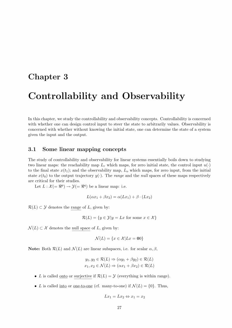
Chapter 3
Controllability and Observability
In this chapter, we study the controllability and observability concepts. Controllability is concernedwith whether one can design control input to steer the state to arbitrarily values. Observability isconcerned with whether without knowing the initial state, one can determine the state of a systemgiven the input and the output.
3.1 Some linear mapping concepts
The study of controllability and observability for linear systems essentially boils down to studyingtwo linear maps: the reachability map Lr which maps, for zero initial state, the control input u(·)to the final state x(t1); and the observability map, Lo which maps, for zero input, from the initialstate x(t0) to the output trajectory y(·). The range and the null spaces of these maps respectivelyare critical for their studies.
Let L : X (= ℜp) → Y(= ℜq) be a linear map: i.e.
L(αx1 + βx2) = α(Lx1) + β · (Lx2)
R(L) ⊂ Y denotes the range of L, given by:
R(L) = {y ∈ Y|y = Lx for some x ∈ X}
N (L) ⊂ X denotes the null space of L, given by:
N (L) = {x ∈ X |Lx = 00}
Note: Both R(L) and N (L) are linear subspaces, i.e. for scalar α, β,
y1, y2 ∈ R(L) ⇒ (αy1 + βy2) ∈ R(L)
x1, x2 ∈ N (L) ⇒ (αx1 + βx2) ∈ R(L)
• L is called onto or surjective if R(L) = Y (everything is within range).
• L is called into or one-to-one (cf. many-to-one) if N (L) = {0}. Thus,
Lx1 = Lx2 ⇔ x1 = x2
27
28 c©Perry Y.Li
3.1.1 The Finite Rank Theorem
Proposition 3.1.1 : Let L ∈ ℜn×m, so that L : u ∈ ℜm 7→ y ∈ ℜn.
1.R(L) = R(LLT )
2.N (L) = N (LTL)
3. Any point u ∈ ℜn can be written as
u = LT y1 + un ∈ ℜn;where y1 ∈ ℜn, Lun = 0.
In other words, u can always be written as a sum of u1 ∈ R(LT ) and un ∈ N (L).
4. Similarly, any point u ∈ ℜn can be written as
y = Lu1 + yn ∈ ℜn; where u1 ∈ ℜm, LT yn = 0.
In other words, u can always be written as a sum of y1 ∈ R(L) and yn ∈ N (LT ).
Note:
• If L ∈ ℜn×m and m > n (short and fat), then LLT ∈ ℜn×n is both short and thin.
• To check whether the system is controllable we need to check if LLT is full rank - e.g. checkits determinant.
• If m < n (tall and thin), then LTL ∈ ℜn×n is also both short and thin.
• Checking N (LTL) will be useful when we talk about observerability.
3.2 Controllability
Consider a state determined dynamical system with a transition map s(t1, t0, x0, u(·)) such that
x(t1) = s(t1, t0, x(t0), u(·)).
This can be continuous time or discrete time.
Definition 3.2.1 (Controllability) : The dynamical system is controllable on [t0, t1] if ∀ initialand final states x0, x1, ∃u(·) so that s(t1, t0, x0, u) = x1.
It is said to controllable at t0 if ∀x0, x1, ∃t1 ≥ t0 and u(·) ∈ U so that s(t1, t0, x0, u) = x1
A system that is not controllable probably means the followings:
• If state space system is realized from input-output data, then the realization is redundant.i.e. some states have no relationship to either the input or the output.
• If states are meaningful (physical) variables that need to be controlled, then the design of theactuators are deficient.
• The effect of control is limited. There is also a possibililty of instability
ME 8281:Advanced Control Systems, F01, F02, S06, S08 29
Remarks:
• The followings are equivalent:
1. A system is controllable at t = t0.
2. The system can be transferred from any state at t = t0 to any other state in finite time.
3. For each x0 ∈ Σ,
s(·, t0, x0, ·) : [t0,∞) × u(·) 7→ s(t1, t0, x0, u(·))
is surjective (onto).
• Controllability does not say that x(t) remains at x1. e.g. for
x = Ax+Bu
to make x(t) = x1 ∀t ≥ t0, it is necessary that Ax1 ∈ Range(B). This is generally not true.
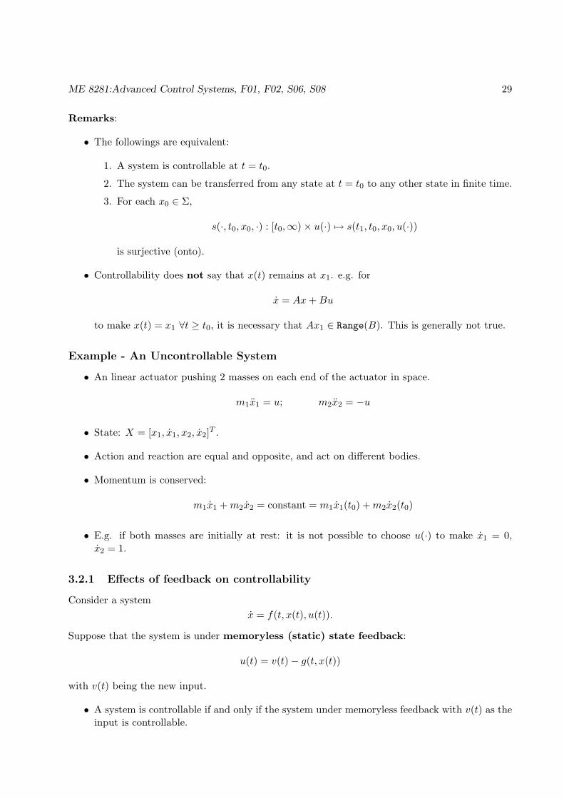
Example - An Uncontrollable System
• An linear actuator pushing 2 masses on each end of the actuator in space.
m1x1 = u; m2x2 = −u
• State: X = [x1, x1, x2, x2]T .
• Action and reaction are equal and opposite, and act on different bodies.
• Momentum is conserved:
m1x1 +m2x2 = constant = m1x1(t0) +m2x2(t0)
• E.g. if both masses are initially at rest: it is not possible to choose u(·) to make x1 = 0,x2 = 1.
3.2.1 Effects of feedback on controllability
Consider a system
x = f(t, x(t), u(t)).
Suppose that the system is under memoryless (static) state feedback:
u(t) = v(t) − g(t, x(t))
with v(t) being the new input.
• A system is controllable if and only if the system under memoryless feedback with v(t) as theinput is controllable.
30 c©Perry Y.Li
Proof: Suppose that the original system is controllable. Given a pair of initial and final states,x0 and x1, suppose that the control u(·) transfers the state from x0 at t0 to x1 at t1. For the newsystem, which has also x(t) as the state variables, we can use the control v(t) = u(t) + g(t, x(t)) totransfer the state from x0 at t0 to x1 at t1. Therefore, the new system is also controllable.
Suppose that the feedback system is controllable, and v(·) is the control that can achieve thedesired state transfer. Then for the original system, we can use the control u(t) = v(t) − g(t, x(t))to achieve the same state transfer. Thus, the original system is also controllable. ⋄
Consider now the system under dynamic state feedback:
z(t) = α(t, x(t), z(t))
u(t) = v(t) − g(t, x(t), z(t))
where v(t) is the new input and z(t) is the state of the controller.
• If a system under dynamic feedback is controllable then the original system is.
• The converse is not true, i.e. the original system is controllable does not necessarily implythat the system under dynamic state feedback is.
Proof: The same proof for the memoryless state feedback works for the first statement. For thesecond statement, we give an example of the controller:
z = z; u(t) = v(t) − g(t, x(t), z(t)).
The state of the new system is (x, z) but no control can affect z(t). Thus, the new system is notcontrollable. ⋄These results show that feedback control cannot make a uncontrollable system become controllable,but can even make a controllable system, uncontrollable. To make a system controllable, one mustredesign the actuators.
3.3 Controllability of Linear Systems
Continuous time system:
x(t) = A(t)x(t) +B(t)u(t) x ∈ ℜn
x(t1) = Φ(t1, t0)x0 +
∫ t1
t0
Φ(t1, t)B(t)u(t)dt.
The reachability map on [t0, t1] is defined to be:
Lr,[t0,t1](u(·)) =
∫ t1
t0
Φ(t1, t)B(t)u(t)dt
Thus, it is controllable on [t0, t1] if and only if Lr,[t0,t1](u(·)) is surjective (onto).Notice that Lr,[t0,t1] determines the set of states that can be reached from the origin at t = t1.The study of the range space of the linear map:
Lr,[t0,t1] : {u(·)} → ℜn
is central to the study of controllability.
ME 8281:Advanced Control Systems, F01, F02, S06, S08 31
Proposition 3.3.1 If a continuous time, possibly time varying, linear system is controllable on[t0, t1] then it is controllable on [t0, t2] where t2 ≥ t1.
Proof: To transfer from x(t0) = x0 to x(t2) = x2, define
x1 = Φ(t1, t2)x2
Suppose that u∗[t0,t1] transfers x(t0) = x0 to x(t1) = x1. Choose
u(t) =
{
u∗(t) t ∈ [t0, t1]
0 t ∈ (t1, t2]
⋄. ⋄
This result does not hold for t0 < t2 < t1. e.g. The system
x(t) = B(t)u(t) B(t) =
{
0 t ∈ [t0, t2]
In t ∈ (t2, t1].
is controllable on [t0, t1] but x(t2) = x(t0) for any control u(·).
3.3.1 Discrete time system
x(k + 1) = A(k)x(k) +B(k)u(k), x ∈ ℜn, u ∈ ℜm
x(k1) = Φ(k1, k0)x(k0) +
k1−1∑
k=k0
Φ(k1, k + 1)B(k)u(k)
The transition function of the discrete time system is given by:
x(k1) = s(k0, k1, x(k0), u(·)) = Φ(k1, k0)x(k0) +
k1−1∑
k=k0
Φ(k1, k + 1)B(k)u(k) (3.1)
Φ(kf , ki) = Πkf−1k=ki
A(k) (3.2)
The reachability map of the discrete time system can be written as:
Lr,[k0,k1](u(k0), . . . , u(k1 − 1)) =
k1−1∑
k=k0
Φ(k1, k + 1)B(k)u(k) = Lr(k0, k1)U
where Lr(k0, k1) ∈ ℜn×(k1−k0)m, U =
u(k0)...
u(k1 − 1)
.
Thus, the system is controllable on [k0, k1] if and only if Lr,[k0,k1] is surjective, which is true ifand only if Lr(k0, k1) has rank n
Proposition 3.3.2 Suppose that A(k) is nonsingular for each k1 ≤ k < k2, then the discrete timelinear system is controllable on [k0, k1] implies that it is controllable on [k0, k2] where k2 ≥ k1.
Proof: : The proof is similar to the continuous case. However for a discrete time system, we needA(k) nonsingular for k1 ≤ k < k2 to ensure that Φ(k2, k1) is invertible. Q.E.D. ⋄
32 c©Perry Y.Li
Example
Consider a unit point mass under control of a force:
d
dt
(xx
)
=
(0 10 0
)(xx
)
+
(01
)
u
This is the same as x = u.Suppose that x(0) = x(0) = 0, we would like to translate the mass to x(T ) = 1, x(T ) = 0.The reachability map L : u(·) → x(T ) is
x(T ) =
∫ T
0Φ(T, t)B(t)u(t)dt
Let use try to solve this problem using piecewise constant control:
u(t) =
u0 0 ≤ t < T/10
u1 T/10 ≤ t < 2T/10...
u10 9T/10 ≤ t ≤ T
and find U = [u1, u2, . . . , u10]T .
The reachability map becomes:
x(T ) =(L1 L2 . . . L10
)
︸ ︷︷ ︸
Lr
u1
u2...u10
where
L1 =
[∫ T/10
0Φ(T, t)B(t)dt
]
=T
10
(T1
)
,
L2 =
[∫ 2T/10
T/10Φ(T, t)B(t)dt
]
=T
10
(0.9T
1
)
,
...
L10 =T
10
(0.1T
1
)
Whether the matrix denoted by Lr ∈ ℜ2×10 is surjective (onto) (i.e. R(Lr) = ℜ2 determineswhether we can achieve our task using piecewise constant control.
In our case, let T = 10 for convenience,
Lr =
(10 9 . . . 11 1 . . . 1
)
and
LrLTr =
(385 5555 10
)
ME 8281:Advanced Control Systems, F01, F02, S06, S08 33
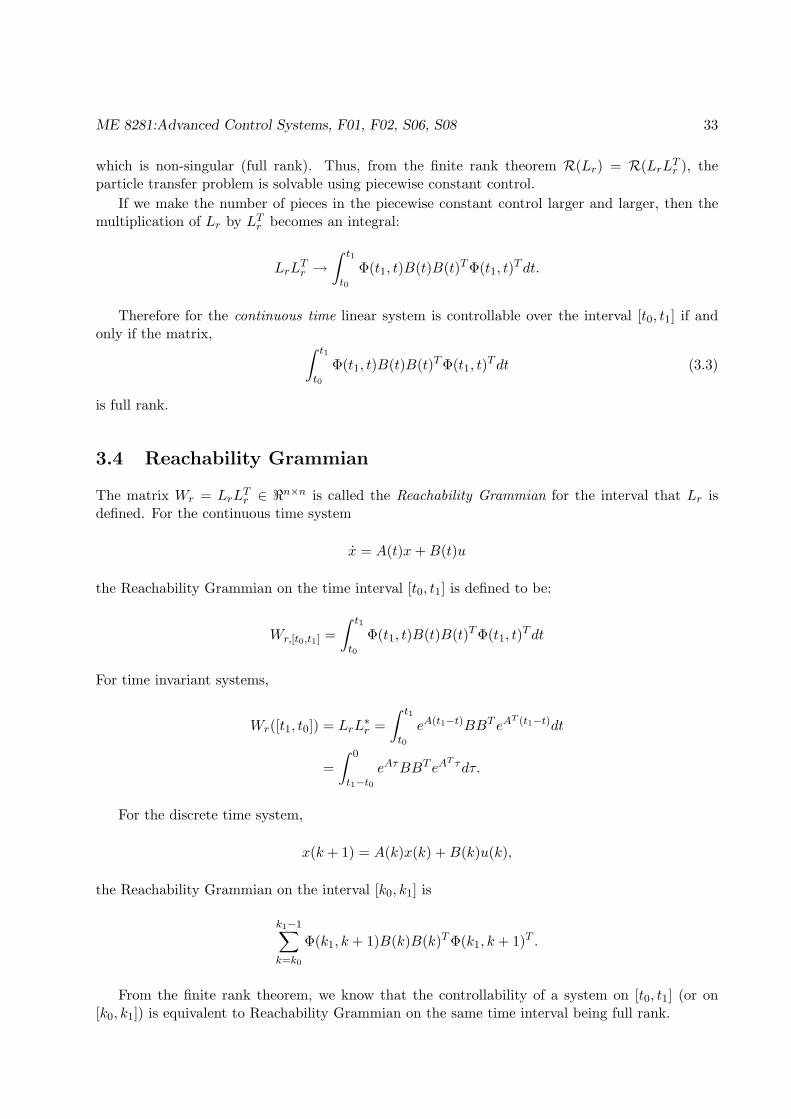
which is non-singular (full rank). Thus, from the finite rank theorem R(Lr) = R(LrLTr ), the
particle transfer problem is solvable using piecewise constant control.
If we make the number of pieces in the piecewise constant control larger and larger, then themultiplication of Lr by LT
r becomes an integral:
LrLTr →
∫ t1
t0
Φ(t1, t)B(t)B(t)T Φ(t1, t)Tdt.
Therefore for the continuous time linear system is controllable over the interval [t0, t1] if andonly if the matrix,
∫ t1
t0
Φ(t1, t)B(t)B(t)T Φ(t1, t)Tdt (3.3)
is full rank.
3.4 Reachability Grammian
The matrix Wr = LrLTr ∈ ℜn×n is called the Reachability Grammian for the interval that Lr is
defined. For the continuous time system
x = A(t)x+B(t)u
the Reachability Grammian on the time interval [t0, t1] is defined to be:
Wr,[t0,t1] =
∫ t1
t0
Φ(t1, t)B(t)B(t)T Φ(t1, t)Tdt
For time invariant systems,
Wr([t1, t0]) = LrL∗r =
∫ t1
t0
eA(t1−t)BBT eAT (t1−t)dt
=
∫ 0
t1−t0
eAτBBT eAT τdτ.
For the discrete time system,
x(k + 1) = A(k)x(k) +B(k)u(k),
the Reachability Grammian on the interval [k0, k1] is
k1−1∑
k=k0
Φ(k1, k + 1)B(k)B(k)T Φ(k1, k + 1)T .
From the finite rank theorem, we know that the controllability of a system on [t0, t1] (or on[k0, k1]) is equivalent to Reachability Grammian on the same time interval being full rank.
34 c©Perry Y.Li
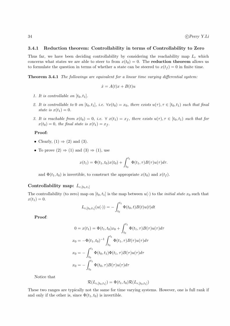
3.4.1 Reduction theorem: Controllability in terms of Controllability to Zero
Thus far, we have been deciding controllability by considering the reachability map Lr whichconcerns what states we are able to steer to from x(t0) = 0. The reduction theorem allows usto formulate the question in terms of whether a state can be steered to x(tf ) = 0 in finite time.
Theorem 3.4.1 The followings are equivalent for a linear time varying differential system:
x = A(t)x+B(t)u
1. It is controllable on [t0, t1].
2. It is controllable to 0 on [t0, t1], i.e. ∀x(t0) = x0, there exists u(τ), τ ∈ [t0, t1) such that finalstate is x(t1) = 0.
3. It is reachable from x(t0) = 0, i.e. ∀ x(t1) = xf , there exists u(τ), τ ∈ [t0, t1) such that forx(t0) = 0, the final state is x(t1) = xf .
Proof:
• Clearly, (1) ⇒ (2) and (3).
• To prove (2) ⇒ (1) and (3) ⇒ (1), use
x(t1) = Φ(t1, t0)x(t0) +
∫ t1
t0
Φ(t1, τ)B(τ)u(τ)dτ.
and Φ(t1, t0) is invertible, to construct the appropriate x(t0) and x(tf ).
Controllability map: Lc,[t0,t1]
The controllability (to zero) map on [t0, t1] is the map between u(·) to the initial state x0 such thatx(t1) = 0.
Lc,[t0,t1](u(·)) = −
∫ t1
t0
Φ(t0, t)B(t)u(t)dt
Proof:
0 = x(t1) = Φ(t1, t0)x0 +
∫ t1
t0
Φ(t1, τ)B(τ)u(τ)dτ
x0 = −Φ(t1, t0)−1
∫ t1
t0
Φ(t1, τ)B(τ)u(τ)dτ
x0 = −
∫ t1
t0
Φ(t0, t1)Φ(t1, τ)B(τ)u(τ)dτ
x0 = −
∫ t1
t0
Φ(t0, τ)B(τ)u(τ)dτ
Notice thatR(Lc,[t0,t1]) = Φ(t1, t0)R(Lr,[t0,t1])
These two ranges are typically not the same for time varying systems. However, one is full rank ifand only if the other is, since Φ(t1, t0) is invertible.
ME 8281:Advanced Control Systems, F01, F02, S06, S08 35
For time invariant continuous time systems, R(Lc,[t0,t1]) = R(Lr,[t0,t1]).The above two statements are not true for time invariant discrete time systems. Can you find
counter-examples?Because of the reduction theorem, the linear continuous time system is controllable on the inter-
val [t0, tf ] if R(Lc,[t0,t1]) = ℜn. From the finite rank theorem, R(Lc,[t0,t1]) = R(Lc,[t0,t1]L∗c,[t0,t1]) =
ℜn. The controllability-to-zero grammian on the time interval [t0, t1] is defined to be:
Wc = LcL∗c =
∫ t1
t0
Φ(t0, t)B(t)B(t)T Φ(t0, t)Tdt
For time invariant system,
Wc = LcL∗c =
∫ t1
t0
eA(t0−t)BBT eAT (t0−t)dt
= −
∫ 0
t1−t0
e−AτBBT e−AT τdτ.
Since controllability of a system on [t0, t1] is equivalent to controllability to 0 which is determinedby the controllability map being surjective, it is also equivalent to controllability grammian on thesame time interval [t0, t1] being full rank.
3.5 Minimum norm control
3.5.1 Formulation
The Controllability Grammian is related to the cost of control.Given x(t0) = x0, find a control function or sequence u(·) so that x(t1) = x1. Let xd =
x1 − Φ(t1, t0)x0. Then we must have
xd = Lr,[t0,t1](u)
where Lr,[t0,t1] : {u(·)} → ℜ is the reachability map which, for continuous time system is:
Lr,[t0,t1](u) =
∫ t1
t0
Φ(t1, t)B(t)u(t)dt.
and for discrete time system:
Lr,[k0,k1](u(·)) =
k1−1∑
k=k0
Φ(k1, k + 1)B(k)u(k) = C(k0, k1)U
where C ∈ ℜn×(k1−k0)m, U =
u(k0)...
u(k1 − 1)
.
Let us focus on the discrete time system.Since xd ∈ Range(Lr,[k0,k1]) for solutions to exist, we assume Range(Lr,[k0,k1]) = ℜn. This implies
that Wr,[k0,k1] is invertible.Generally there are multiple solutions. To resolve the non-uniqueness, we find the solution so
that
J(U) =1
2
k1−1∑
k=k0
u(k)Tu(k) = UTU
is minimized. Here U = [u(k0);u(k0 + 1); . . . ;u(k1 − 1)].
36 c©Perry Y.Li
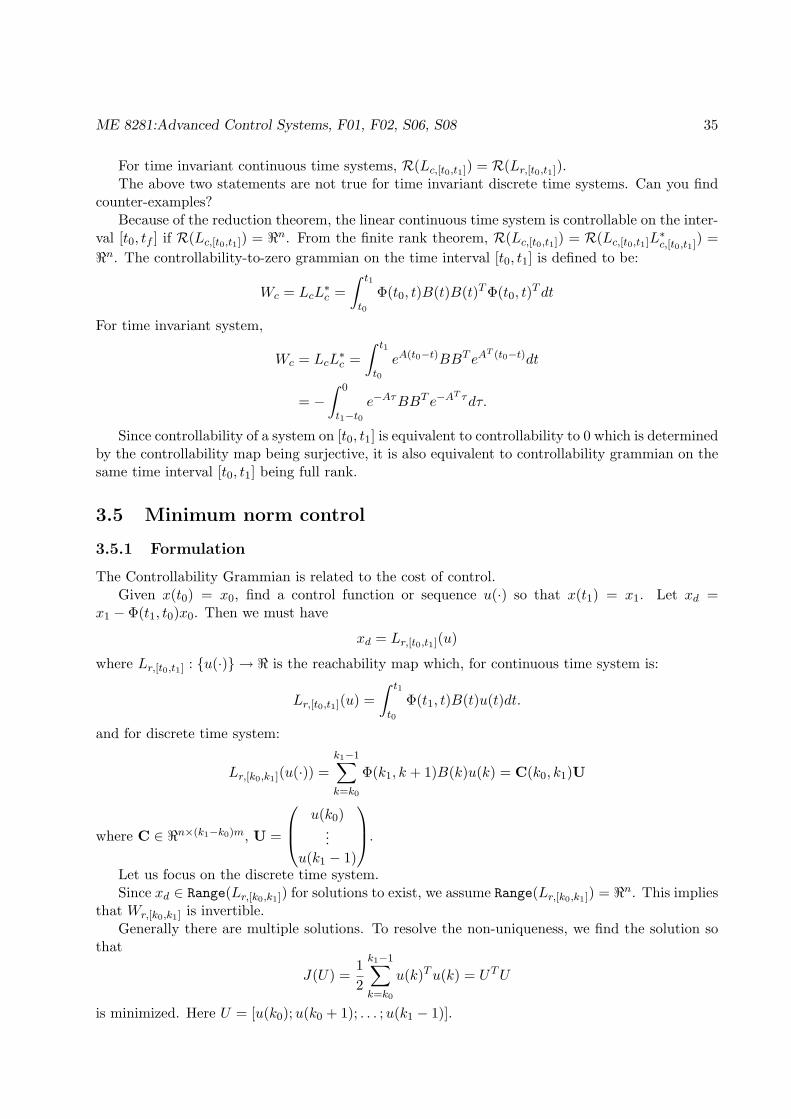
3.5.2 Least norm control solution
This is a constrained optimization problem (with J(U) as the cost to be minimized, and LrU−xd =0 as the constraint). It can be solved using the Lagrange Multiplier method of converting aconstrained optimization problem into an unconstrained optimization.
Define an augmented cost function, with the Lagrange multipliers λ ∈ ℜn
J ′(U, λ) = J(U) + λT (LrU − xd)
The optimal given by (U∗, λ∗) must satisfy:
∂J ′
∂U(U∗, λ∗) = 0;
∂J ′
∂λ(U∗, λ∗) = 0
The second condition is just the constraint: LrU = xd.This means that
LTr λ
∗ + U∗ = 0; LrU∗ = xd
Solving, we get:
λ∗ = −(LrLTr )−1xd = −W−1
r xd
U∗ = −LTr λ
∗ = LTr W
−1r xd.
The optimal cost of control is:
J(U∗) = xTdW
−1r LrL
Tr W
−1r xd = xT
dW−1r xd
Thus, the inverse of the Reachability Grammian tells us how difficult it is to perform a state transferfrom x = 0 to xd. In particular, if Wr is not invertible, for some xd, the cost is infinite.
3.5.3 Geometric interpretation of least norm solution
Geometrically, we can think of the cost as J = UTU , i.e. the inner product of U with itself. Innotation of inner product,
J =< U,U >R
The advantage of the notation is that we can change the definition of inner product, e.g. <U, V >R= UTRV where R is a positive definite matrix. The usual inner (dot) product has R = I.
We say that U and V are normal to each other if < U, V >R= 0.Any solution that satisfies the constraint must be of the form
(U − Up) ∈ Null(Lr)
where LrUp = xf is any particular solution.
Claim: Let U∗ be the optimal solution, and U is any solution that satisfies the constraint. Then,(U − U∗) ⊥ U∗, i.e.
< (U − U∗), U∗ >R= 0
which is the normal equation for the least norm solution problem.Proof: Direct substitution.
(U − U∗)TRUR−1U LT
pc
(LrR
−1U LT
r
)−1xf = (Lr(U − U∗))T (
LrR−1U LT
r
)−1xf = 0.
⋄
ME 8281:Advanced Control Systems, F01, F02, S06, S08 37
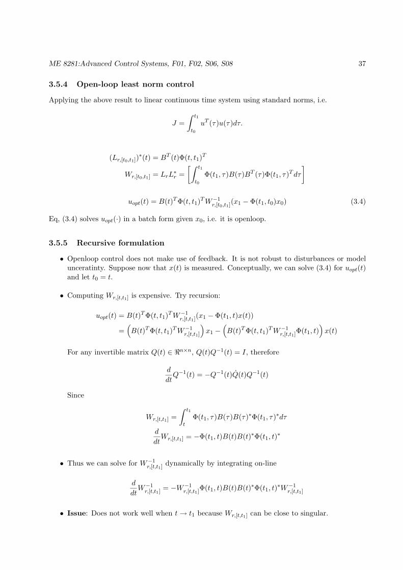
3.5.4 Open-loop least norm control
Applying the above result to linear continuous time system using standard norms, i.e.
J =
∫ t1
t0
uT (τ)u(τ)dτ.
(Lr,[t0,t1])∗(t) = BT (t)Φ(t, t1)
T
Wr,[t0,t1] = LrL∗r =
[∫ t1
t0
Φ(t1, τ)B(τ)BT (τ)Φ(t1, τ)Tdτ
]
uopt(t) = B(t)T Φ(t, t1)TW−1
r,[t0,t1](x1 − Φ(t1, t0)x0) (3.4)
Eq, (3.4) solves uopt(·) in a batch form given x0, i.e. it is openloop.
3.5.5 Recursive formulation
• Openloop control does not make use of feedback. It is not robust to disturbances or modelunceratinty. Suppose now that x(t) is measured. Conceptually, we can solve (3.4) for uopt(t)and let t0 = t.
• Computing Wr,[t,t1] is expensive. Try recursion:
uopt(t) = B(t)T Φ(t, t1)TW−1
r,[t,t1](x1 − Φ(t1, t)x(t))
=(
B(t)T Φ(t, t1)TW−1
r,[t,t1]
)
x1 −(
B(t)T Φ(t, t1)TW−1
r,[t,t1]Φ(t1, t))
x(t)
For any invertible matrix Q(t) ∈ ℜn×n, Q(t)Q−1(t) = I, therefore
d
dtQ−1(t) = −Q−1(t)Q(t)Q−1(t)
Since
Wr,[t,t1] =
∫ t1
tΦ(t1, τ)B(τ)B(τ)∗Φ(t1, τ)
∗dτ
d
dtWr,[t,t1] = −Φ(t1, t)B(t)B(t)∗Φ(t1, t)
∗
• Thus we can solve for W−1r,[t,t1] dynamically by integrating on-line
d
dtW−1
r,[t,t1] = −W−1r,[t,t1]Φ(t1, t)B(t)B(t)∗Φ(t1, t)
∗W−1r,[t,t1]
• Issue: Does not work well when t→ t1 because Wr,[t,t1] can be close to singular.
38 c©Perry Y.Li
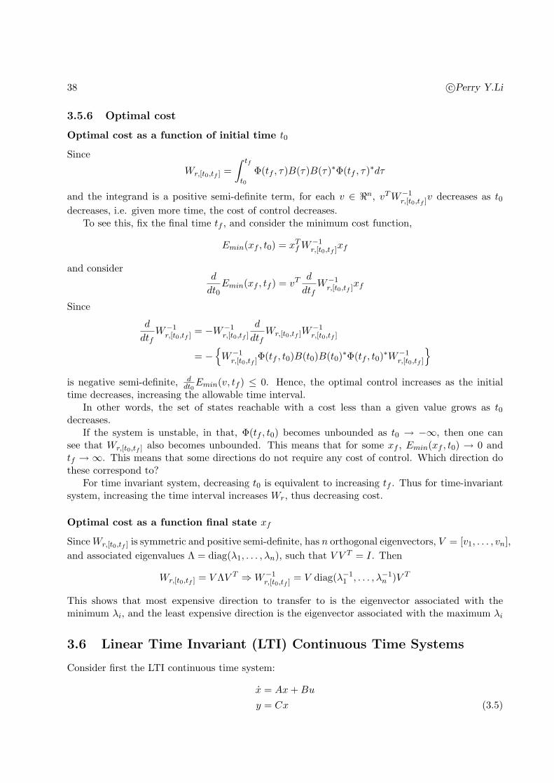
3.5.6 Optimal cost
Optimal cost as a function of initial time t0
Since
Wr,[t0,tf ] =
∫ tf
t0
Φ(tf , τ)B(τ)B(τ)∗Φ(tf , τ)∗dτ
and the integrand is a positive semi-definite term, for each v ∈ ℜn, vTW−1r,[t0,tf ]v decreases as t0
decreases, i.e. given more time, the cost of control decreases.To see this, fix the final time tf , and consider the minimum cost function,
Emin(xf , t0) = xTf W
−1r,[t0,tf ]xf
and considerd
dt0Emin(xf , tf ) = vT d
dtfW−1
r,[t0,tf ]xf
Since
d
dtfW−1
r,[t0,tf ] = −W−1r,[t0,tf ]
d
dtfWr,[t0,tf ]W
−1r,[t0,tf ]
= −{
W−1r,[t0,tf ]Φ(tf , t0)B(t0)B(t0)
∗Φ(tf , t0)∗W−1
r,[t0,tf ]
}
is negative semi-definite, ddt0Emin(v, tf ) ≤ 0. Hence, the optimal control increases as the initial
time decreases, increasing the allowable time interval.In other words, the set of states reachable with a cost less than a given value grows as t0
decreases.If the system is unstable, in that, Φ(tf , t0) becomes unbounded as t0 → −∞, then one can
see that Wr,[t0,tf ] also becomes unbounded. This means that for some xf , Emin(xf , t0) → 0 andtf → ∞. This means that some directions do not require any cost of control. Which direction dothese correspond to?
For time invariant system, decreasing t0 is equivalent to increasing tf . Thus for time-invariantsystem, increasing the time interval increases Wr, thus decreasing cost.
Optimal cost as a function final state xf
SinceWr,[t0,tf ] is symmetric and positive semi-definite, has n orthogonal eigenvectors, V = [v1, . . . , vn],
and associated eigenvalues Λ = diag(λ1, . . . , λn), such that V V T = I. Then
Wr,[t0,tf ] = V ΛV T ⇒W−1r,[t0,tf ] = V diag(λ−1
1 , . . . , λ−1n )V T
This shows that most expensive direction to transfer to is the eigenvector associated with theminimum λi, and the least expensive direction is the eigenvector associated with the maximum λi
3.6 Linear Time Invariant (LTI) Continuous Time Systems
Consider first the LTI continuous time system:
x = Ax+Bu
y = Cx (3.5)
ME 8281:Advanced Control Systems, F01, F02, S06, S08 39
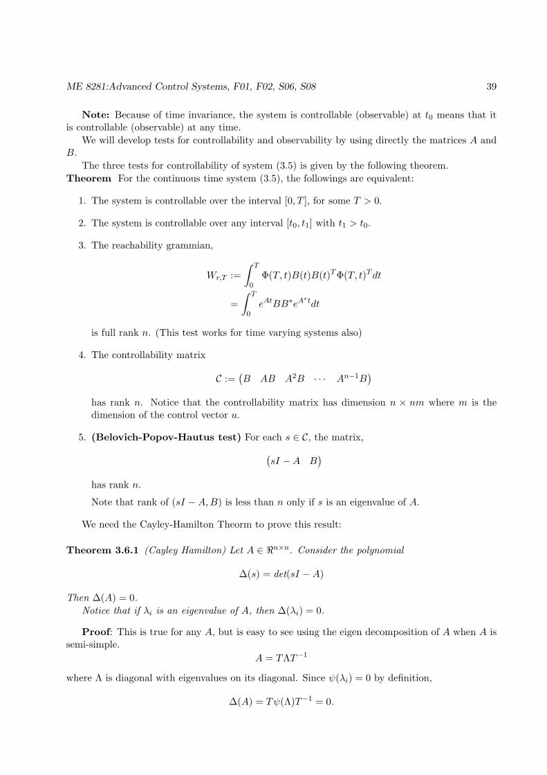
Note: Because of time invariance, the system is controllable (observable) at t0 means that itis controllable (observable) at any time.
We will develop tests for controllability and observability by using directly the matrices A andB.
The three tests for controllability of system (3.5) is given by the following theorem.
Theorem For the continuous time system (3.5), the followings are equivalent:
1. The system is controllable over the interval [0, T ], for some T > 0.
2. The system is controllable over any interval [t0, t1] with t1 > t0.
3. The reachability grammian,
Wr,T :=
∫ T
0Φ(T, t)B(t)B(t)T Φ(T, t)Tdt
=
∫ T
0eAtBB∗eA
∗tdt
is full rank n. (This test works for time varying systems also)
4. The controllability matrix
C :=(B AB A2B · · · An−1B
)
has rank n. Notice that the controllability matrix has dimension n × nm where m is thedimension of the control vector u.
5. (Belovich-Popov-Hautus test) For each s ∈ C, the matrix,
(sI −A B
)
has rank n.
Note that rank of (sI −A,B) is less than n only if s is an eigenvalue of A.
We need the Cayley-Hamilton Theorm to prove this result:
Theorem 3.6.1 (Cayley Hamilton) Let A ∈ ℜn×n. Consider the polynomial
∆(s) = det(sI −A)
Then ∆(A) = 0.
Notice that if λi is an eigenvalue of A, then ∆(λi) = 0.
Proof: This is true for any A, but is easy to see using the eigen decomposition of A when A issemi-simple.
A = TΛT−1
where Λ is diagonal with eigenvalues on its diagonal. Since ψ(λi) = 0 by definition,
∆(A) = Tψ(Λ)T−1 = 0.
40 c©Perry Y.Li
Proof: Controllability test(1) ⇐⇒ (3): We have already seen before that controllability over the interval [0, T ] means thatthe range space of the reachability map,
Lr(u) =
∫ T
0eA(T−τ)Bu(τ)dτ
must be the whole state space, ℜn. Notice that
Wr,T :=
∫ T
0eAtBB∗eA
∗tdt = LrL∗r
where L∗r is the adjoint (think transpose) of Lr.
From the finite rank linear map theorem, R(Lr) = R(LrL∗r) but, LrL
∗r is nothing but Wr,T .
(3) ⇒ (4): We will show this by showing “not (4) ⇒ not (3)”. Suppose that (4) is not true.Then, there exists a 1 × n vector vT so that,
vTB = vTAB = vTA2B · · · = vTAn−1B = 0.
Consider now,
vTWr,T v =
∫ T
0‖vT eAtB‖2
2dt.
Since
eAt = I +At+A2t2
2+An−1tn−1
n− 1!+ · · ·
and by the Cayley Hamilton Theorem, Ak is a linear combination of I, A, ... An−1, therefore,
vT eAtB = 0
for all t. Hence, vTWr,T v = 0 or Wr,T is not full rank.
(3) ⇒ (2): We will show this by showing “not (2) ⇒ not (3)”. If (2) is not true, then thereexists 1 × n vector vT so that
vTWr,T v =
∫ T
0‖vT eAtB‖2
2dt = 0.
Because eAt is continuous in t, this implies that vT eAtB = 0 for all t ∈ [0, T ] .
Hence, the all time derivatives of vT eAtB = 0 for all t ∈ [0, T ]. In particular, at t = 0,
vT eAtB |t=0 = vTB = 0
vT d
dteAtB |t=0 = vTAB = 0
vT d2
dt2eAtB |t=0 = vTA2B = 0
...
vT dn−1
dtn−1eAtB |t=0 = vTAn−1B = 0
ME 8281:Advanced Control Systems, F01, F02, S06, S08 41
Hence,
vT(B AB A2B · · · An−1B
)=
(0 0 · · · 0
)
i.e. the controllability matrix of (A,B) is not full rank.
(4) ⇒ (5): We will show “ not (5) implies not (4)”. Suppose (5) is not true so that there exists a1 × n vector v, and λ ∈ C,
vT (λI −A) = 0, vTB = 0.
for some λ. Then vTA = λvT , vTA2 = λ2vT etc. Because vTB = 0 by assumption, we havevTAB = λvTB = 0, vTA2B = λ2vTB = 0 etc. Hence,
vTB = vTAB = vTA2B = · · · vTAn−1B = 0.
Therefore the controllability is not full rank.
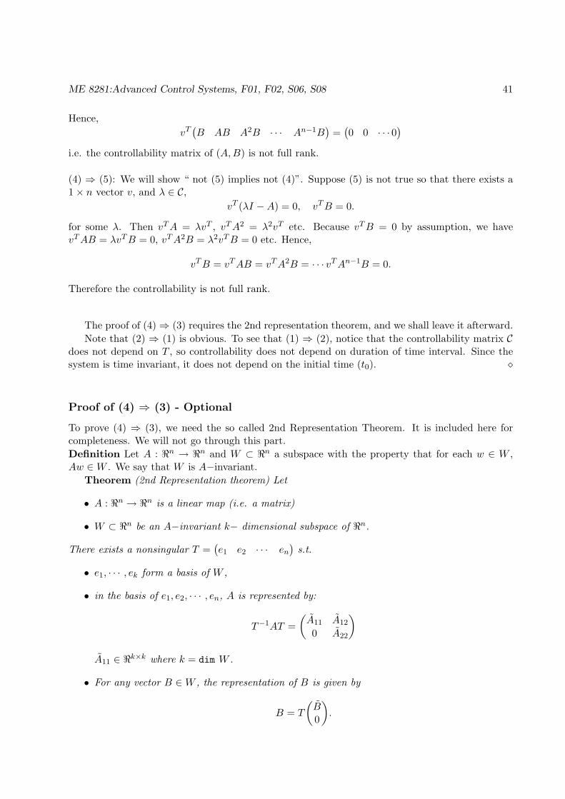
The proof of (4) ⇒ (3) requires the 2nd representation theorem, and we shall leave it afterward.
Note that (2) ⇒ (1) is obvious. To see that (1) ⇒ (2), notice that the controllability matrix Cdoes not depend on T , so controllability does not depend on duration of time interval. Since thesystem is time invariant, it does not depend on the initial time (t0). ⋄
Proof of (4) ⇒ (3) - Optional
To prove (4) ⇒ (3), we need the so called 2nd Representation Theorem. It is included here forcompleteness. We will not go through this part.
Definition Let A : ℜn → ℜn and W ⊂ ℜn a subspace with the property that for each w ∈ W ,Aw ∈W . We say that W is A−invariant.
Theorem (2nd Representation theorem) Let
• A : ℜn → ℜn is a linear map (i.e. a matrix)
• W ⊂ ℜn be an A−invariant k− dimensional subspace of ℜn.
There exists a nonsingular T =(e1 e2 · · · en
)s.t.
• e1, · · · , ek form a basis of W ,
• in the basis of e1, e2, · · · , en, A is represented by:
T−1AT =
(A11 A12
0 A22
)
A11 ∈ ℜk×k where k = dim W .
• For any vector B ∈W , the representation of B is given by
B = T
(B0
)
.
42 c©Perry Y.Li
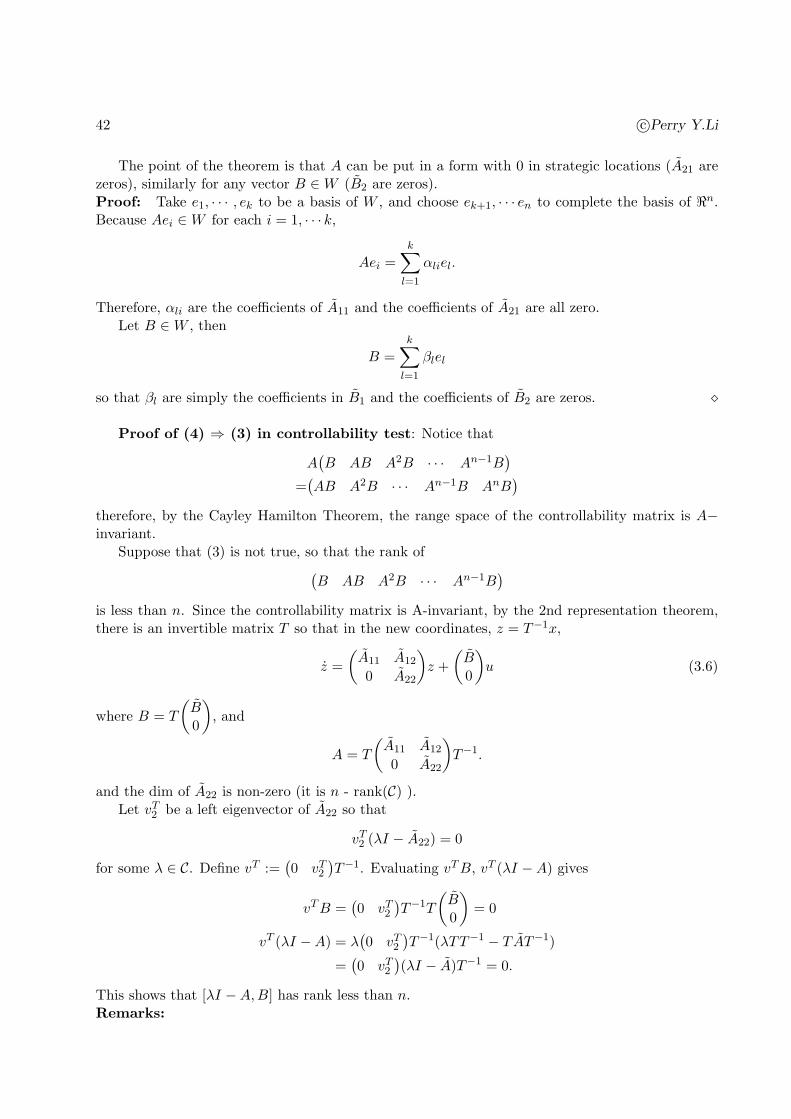
The point of the theorem is that A can be put in a form with 0 in strategic locations (A21 arezeros), similarly for any vector B ∈W (B2 are zeros).Proof: Take e1, · · · , ek to be a basis of W , and choose ek+1, · · · en to complete the basis of ℜn.Because Aei ∈W for each i = 1, · · · k,
Aei =k∑
l=1
αliel.
Therefore, αli are the coefficients of A11 and the coefficients of A21 are all zero.Let B ∈W , then
B =k∑
l=1
βlel
so that βl are simply the coefficients in B1 and the coefficients of B2 are zeros. ⋄
Proof of (4) ⇒ (3) in controllability test: Notice that
A(B AB A2B · · · An−1B
)
=(AB A2B · · · An−1B AnB
)
therefore, by the Cayley Hamilton Theorem, the range space of the controllability matrix is A−invariant.
Suppose that (3) is not true, so that the rank of(B AB A2B · · · An−1B
)
is less than n. Since the controllability matrix is A-invariant, by the 2nd representation theorem,there is an invertible matrix T so that in the new coordinates, z = T−1x,
z =
(A11 A12
0 A22
)
z +
(B0
)
u (3.6)
where B = T
(B0
)
, and
A = T
(A11 A12
0 A22
)
T−1.
and the dim of A22 is non-zero (it is n - rank(C) ).Let vT
2 be a left eigenvector of A22 so that
vT2 (λI − A22) = 0
for some λ ∈ C. Define vT :=(0 vT
2
)T−1. Evaluating vTB, vT (λI −A) gives
vTB =(0 vT
2
)T−1T
(B0
)
= 0
vT (λI −A) = λ(0 vT
2
)T−1(λTT−1 − TAT−1)
=(0 vT
2
)(λI − A)T−1 = 0.
This shows that [λI −A,B] has rank less than n.Remarks:

ME 8281:Advanced Control Systems, F01, F02, S06, S08 43
1. Notice that the controllability matrix is not a function of the time interval. Hence, if a LTIsystem is controllable over some interval, it is controllable over any (non-zero) interval. c.f.with result of linear time varying system.
2. Because of the above fact, we often say that the pair (A,B) is controllable.
3. Controllability test can be done by just examining A and B without computing the grammian.The test in (4) is attractive in that it enumerates the vectors in the controllability subspace.However, numerically, since it involves power of A, numerical stability needs to be considered.
4. The PBH Test in (5), or the Hautus test for short, involves simply checking the condition atthe eigenvalues. It is because for (sI−A,B) to have rank less than n, s must be an eigenvalue.
5. The range space of the controllability matrix is of special interests. It is called the control-lable subspace and is the set of all states that can be reached from zero-initial condition.This is A− invariant.
6. Using the basis for the controllable subspace as part of the basis for ℜn, the controllabilityproperty can be easily seen in (3.6).
3.7 Linear Time Invariant (LTI) discrete time system
For the discrete time system (3.7),
x(k + 1) = Ax(k) +Bu(k)
y(k) = Cx(k) (3.7)
where x ∈ ℜn, u ∈ ℜm, the conditions for controllability is fairly similar except that we need toconsider controllability over period of length greater than n.
First, recall that the reachability map for a linear discrete time system Lr,[k,k1] : u(·) 7→s(k, k0, x = 0, u(·)) is given by:
Lr,[k0,k1][u(·)] =k−1∑
i=k0
Πk−1j=i+1A(j)B(i)u(i) (3.8)
Theorem For the discrete time system (3.7), the followings are equivalent:
1. The system is controllable over the interval [0, T ], with T ≥ n (i.e. it can transfer from anyarbitrary state at k = 0 to any other arbitrary state at k = T ).
2. The system is controllable over the interval [k0, k1], with k1 − k0 ≥ n
3. The controllability grammian,
Wr,T :=T−1∑
l=0
AlBB∗A∗l
is full rank n.
4. The controllability matrix(B AB A2B · · · An−1B
)
has rank n. Notice that the controllability matrix has dimension n × nm where m is thedimension of the control vector u.
44 c©Perry Y.Li
5. For each z ∈ C, the matrix,(zI −A B
)
has rank n.
Proof: The proof of this theorem is exactly analogous to the continuous time case. However, inthe case of the equivalence of (2) and (3), we can notice that
x(k) = Akx(0) + [B,AB,A2B, · · ·An−1B]
u(k − 1)u(k − 2)
...u(0)
so clearly one can transfer to arbitrary states at k = n iff the controllability matrix is full rank.Controllability does not improve for T > n is again the consequence of Cayley-Hamilton Theorem. ⋄
3.8 Observability
The observability question deals with the question of while not knowing the initial state, whetherone can determine the state from the input and output. This is equivalent to the question ofwhether one can determine the initial state x(0) when given the input u(t), t ∈ [0, T ] and theoutput y(t), t ∈ [0, T ].
Definition 3.8.1 A state determined dynamical system is called observable on [t0, t1] if for allinputs, u(τ), and outputs y(τ), τ ∈ [t0, t1], the state x(t0) = x0 can be uniquely determined.
For observability, the null space of the observability map on the interval [t0, t1], given by:
Lo : x0 7→ y(·) = C(·)Φ(·, t0)x0, y(τ) = C(τ)Φ(τ, t0)x0Φ(τ, 0)x, ∀τ ∈ [t0, t1]
must be trivial (i.e. only contains 0). Otherwise, if Lo(xn)(t) = y(t) = 0, for all t ∈ [0, T ], then forany α ∈ ℜ,
y(t) = C(t)Φ(t, 0)x = Φ(t, 0)(x+ αxn).
Recall from the finite rank theorem that if the observability map Lo is a matrix, then the nullspace of Lo, N (Lo) = N (LT
o Lo). For continuous time system, Lo can be thought of as an infinitelylong matrix, then the matrix product operation in LT
o Lo becomes an integral, and is written asL∗
oLo where L∗ denotes the adjoint of the L.
The observability Grammian is given by:
Wo,[t0,t1] = L∗oLo =
∫ t1
t0
Φ(t, t0)TCT (t)C(t)Φ(t, t0) ∈ ℜn×n
where L∗o is the adjoint (think transpose) of the observability map.
ME 8281:Advanced Control Systems, F01, F02, S06, S08 45
3.9 Least square estimation
3.9.1 Formulation and solution
Consider the continuous time varying system:
x(t) = A(t)x(t) y(t) = C(t)x(t).
The observability map on [0, t1] is given by: ∀τ ∈ [0, t1]
Lo : x(0) 7→ y(τ) = C(τ)Φ(τ, 0)x(0) (3.9)
The so-called Least squares estimate of x(0) given the output y(τ), τ ∈ [0, t1] is:
x(0|t1) = arg minx0
∫ t1
0eT (τ)e(τ)dτ.
The least squares estimation problem can be cast into a set of linear equations. For example, wecan stack all the outputs y(t), t ∈ [0, t1] into a vector Y = [Y (0), . . . , Y (0.1), . . . , Y (0.2), . . . , Y (t1)]
T ∈ℜpp, and represent Lo as a matrix ∈ ℜpp×n, then,
Y = Lox0 + E;
x∗o = argminx0ETE = (LT
o Lo)−1LT
o Y
Here, E = [E(0), . . . , E(t1)]T = ℜpp is the modeling error or noise. The optimal estimate x∗0 uses
the minimum amount of noise E to explain the data Y .
Notice that the resulting E satisfies ETLo = 0, i.e. E is normal to Range(Lo).
Using the observability map for the LTI continuous time system (3.9) as Lo,
x(0|t1) = W−1o (t1)
∫ t1
0ΦT (τ, 0)CT (τ)y(τ)dτ
Wo(t1) = L∗oLo =
∫ t1
0ΦT (τ, 0)CT (τ)C(τ)Φ(τ, 0)dτ.
One can also find estimates of the states at time t2 given data up to time t1:
x(t2|t1) = Φ(t2, 0)x(0|t1)
This refers to three classes of esimation problems:
• t2 < t1: Filtering problem
• t2 > t1: Prediction problem
• t2 = t1: Observer problem
The estimate x(t|t) is especially useful for control systems as it allows us to effective do statefeedback control.
46 c©Perry Y.Li
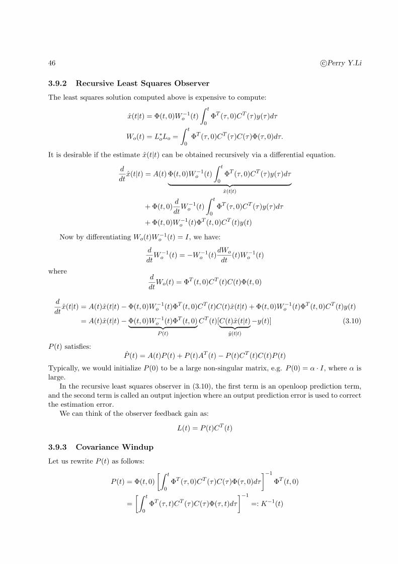
3.9.2 Recursive Least Squares Observer
The least squares solution computed above is expensive to compute:
x(t|t) = Φ(t, 0)W−1o (t)
∫ t
0ΦT (τ, 0)CT (τ)y(τ)dτ
Wo(t) = L∗oLo =
∫ t
0ΦT (τ, 0)CT (τ)C(τ)Φ(τ, 0)dτ.
It is desirable if the estimate x(t|t) can be obtained recursively via a differential equation.
d
dtx(t|t) = A(t)Φ(t, 0)W−1
o (t)
∫ t
0ΦT (τ, 0)CT (τ)y(τ)dτ
︸ ︷︷ ︸
x(t|t)
+ Φ(t, 0)d
dtW−1
o (t)
∫ t
0ΦT (τ, 0)CT (τ)y(τ)dτ
+ Φ(t, 0)W−1o (t)ΦT (t, 0)CT (t)y(t)
Now by differentiating Wo(t)W−1o (t) = I, we have:
d
dtW−1
o (t) = −W−1o (t)
dWo
dt(t)W−1
o (t)
whered
dtWo(t) = ΦT (t, 0)CT (t)C(t)Φ(t, 0)
d
dtx(t|t) = A(t)x(t|t) − Φ(t, 0)W−1
o (t)ΦT (t, 0)CT (t)C(t)x(t|t) + Φ(t, 0)W−1o (t)ΦT (t, 0)CT (t)y(t)
= A(t)x(t|t) − Φ(t, 0)W−1o (t)ΦT (t, 0)
︸ ︷︷ ︸
P (t)
CT (t)[C(t)x(t|t)︸ ︷︷ ︸
y(t|t)
−y(t)] (3.10)
P (t) satisfies:P (t) = A(t)P (t) + P (t)AT (t) − P (t)CT (t)C(t)P (t)
Typically, we would initialize P (0) to be a large non-singular matrix, e.g. P (0) = α · I, where α islarge.
In the recursive least squares observer in (3.10), the first term is an openloop prediction term,and the second term is called an output injection where an output prediction error is used to correctthe estimation error.
We can think of the observer feedback gain as:
L(t) = P (t)CT (t)
3.9.3 Covariance Windup
Let us rewrite P (t) as follows:
P (t) = Φ(t, 0)
[∫ t
0ΦT (τ, 0)CT (τ)C(τ)Φ(τ, 0)dτ
]−1
ΦT (t, 0)
=
[∫ t
0ΦT (τ, t)CT (τ)C(τ)Φ(τ, t)dτ
]−1
=: K−1(t)
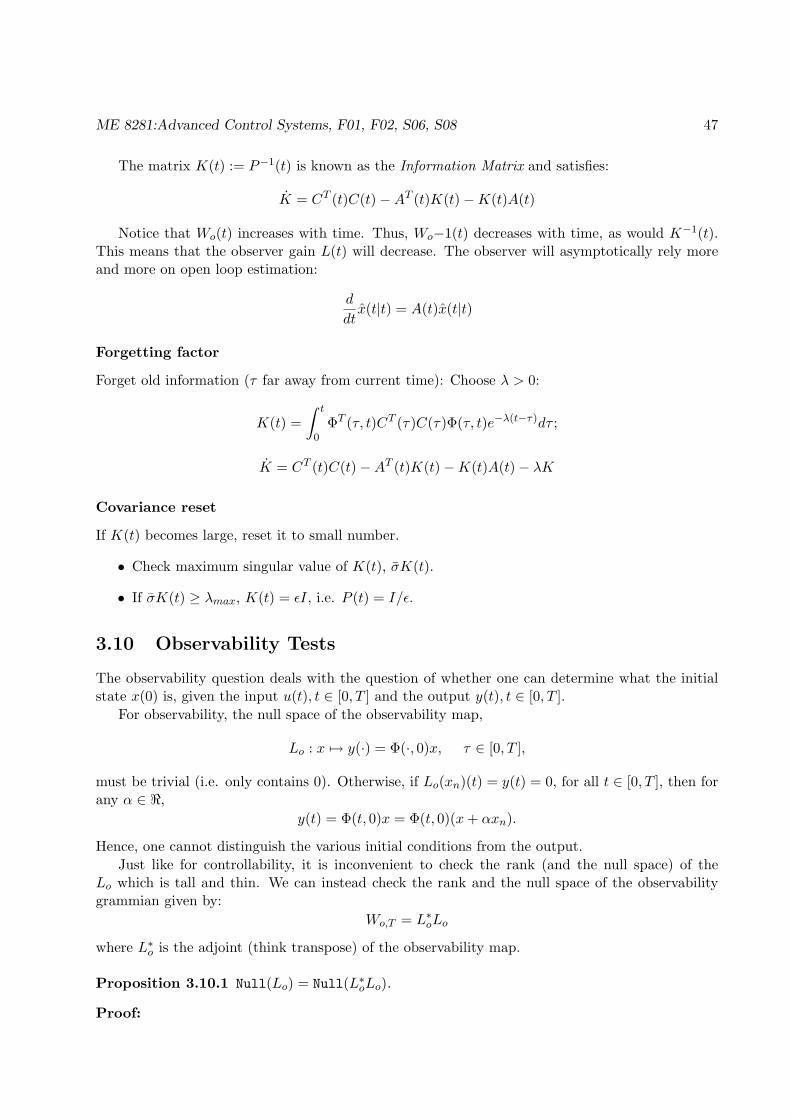
ME 8281:Advanced Control Systems, F01, F02, S06, S08 47
The matrix K(t) := P−1(t) is known as the Information Matrix and satisfies:
K = CT (t)C(t) −AT (t)K(t) −K(t)A(t)
Notice that Wo(t) increases with time. Thus, Wo−1(t) decreases with time, as would K−1(t).This means that the observer gain L(t) will decrease. The observer will asymptotically rely moreand more on open loop estimation:
d
dtx(t|t) = A(t)x(t|t)
Forgetting factor
Forget old information (τ far away from current time): Choose λ > 0:
K(t) =
∫ t
0ΦT (τ, t)CT (τ)C(τ)Φ(τ, t)e−λ(t−τ)dτ ;
K = CT (t)C(t) −AT (t)K(t) −K(t)A(t) − λK
Covariance reset
If K(t) becomes large, reset it to small number.
• Check maximum singular value of K(t), σK(t).
• If σK(t) ≥ λmax, K(t) = ǫI, i.e. P (t) = I/ǫ.
3.10 Observability Tests
The observability question deals with the question of whether one can determine what the initialstate x(0) is, given the input u(t), t ∈ [0, T ] and the output y(t), t ∈ [0, T ].
For observability, the null space of the observability map,
Lo : x 7→ y(·) = Φ(·, 0)x, τ ∈ [0, T ],
must be trivial (i.e. only contains 0). Otherwise, if Lo(xn)(t) = y(t) = 0, for all t ∈ [0, T ], then forany α ∈ ℜ,
y(t) = Φ(t, 0)x = Φ(t, 0)(x+ αxn).
Hence, one cannot distinguish the various initial conditions from the output.
Just like for controllability, it is inconvenient to check the rank (and the null space) of theLo which is tall and thin. We can instead check the rank and the null space of the observabilitygrammian given by:
Wo,T = L∗oLo
where L∗o is the adjoint (think transpose) of the observability map.
Proposition 3.10.1 Null(Lo) = Null(L∗oLo).
Proof:
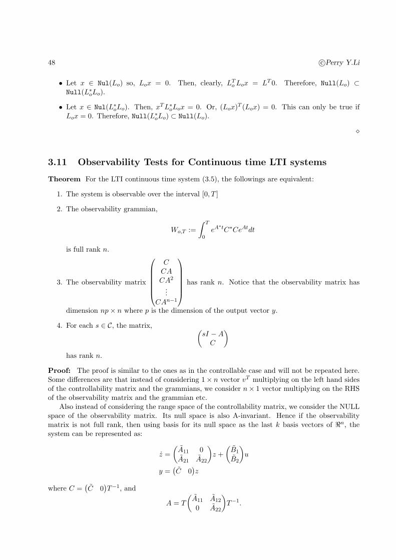
48 c©Perry Y.Li
• Let x ∈ Nul(Lo) so, Lox = 0. Then, clearly, LTo Lox = LT 0. Therefore, Null(Lo) ⊂
Null(L∗oLo).
• Let x ∈ Nul(L∗oLo). Then, xTL∗
oLox = 0. Or, (Lox)T (Lox) = 0. This can only be true if
Lox = 0. Therefore, Null(L∗oLo) ⊂ Null(Lo).
⋄
3.11 Observability Tests for Continuous time LTI systems
Theorem For the LTI continuous time system (3.5), the followings are equivalent:
1. The system is observable over the interval [0, T ]
2. The observability grammian,
Wo,T :=
∫ T
0eA
∗tC∗CeAtdt
is full rank n.
3. The observability matrix
CCACA2
...CAn−1
has rank n. Notice that the observability matrix has
dimension np× n where p is the dimension of the output vector y.
4. For each s ∈ C, the matrix,(sI −AC
)
has rank n.
Proof: The proof is similar to the ones as in the controllable case and will not be repeated here.Some differences are that instead of considering 1× n vector vT multiplying on the left hand sidesof the controllability matrix and the grammians, we consider n× 1 vector multiplying on the RHSof the observability matrix and the grammian etc.
Also instead of considering the range space of the controllability matrix, we consider the NULLspace of the observability matrix. Its null space is also A-invariant. Hence if the observabilitymatrix is not full rank, then using basis for its null space as the last k basis vectors of ℜn, thesystem can be represented as:
z =
(A11 0
A21 A22
)
z +
(B1
B2
)
u
y =(C 0
)z
where C =(C 0
)T−1, and
A = T
(A11 A12
0 A22
)
T−1.
ME 8281:Advanced Control Systems, F01, F02, S06, S08 49
and the dim of A22 is non-zero (and is the dim of the null space of the observability matrix). ⋄
Remark
1. Again, observability of a LTI system does not depend on the time interval. So, theoreticallyspeaking, if observing the output and input for an arbitrary amount of time will be sufficientto figure out x(0). In reality, when more data is available, one can do more averaging toeliminate effects of noise (e.g. using the Least square ie. Kalman Filter approach).
2. The subspace of particular interest is the null space of the controllability matrix. An initialstate lying in this set will generate identically 0 zero-input response. This subspace is calledthe unobservable subspace.
3. Using the basis of the unobservable subspace as part of the basis of ℜn, the observabilityproperty can be easily seen.
3.12 Observability Tests for Discrete time LTI systems
The tests for observability of the discrete time system (3.7) is given similarly by the followingtheorem.
Theorem 3.12.1 For the discrete time system (3.7), the followings are equivalent:
1. The system is observable over the interval [0, T ], for some T ≥ n.
2. The observability grammian,
Wo,T :=T−1∑
k=0
A∗kC∗CAk
is full rank n.
3. The observability matrix
CCACA2
...CAn−1
has rank n. Notice that the observability matrix has
dimension np× n where p is the dimension of the output vector y.
4. For each z ∈ C, the matrix,(zI −AC
)
has rank n.
The controllability matrix can have the following interpretation: zero-input response is givenby:
y(0)y(1)y(2)
...y(n− 1)
=
CCACA2
...CAn−1
x(0).
50 c©Perry Y.Li
Thus, clearly if the observability matrix is full rank, one can reconstruct x(0) from measurementsof y(0), · · · , y(n−1). One might think that by increasing the number of output measurement times(e.g. y(n)) the system can become observable. However, because of Cayley-Hamilton theorem,y(n) = CAnx(0) can be expressed as
∑n−1i=0 aiCA
ix(0) consisting of rows already in the observabilitymatrix.
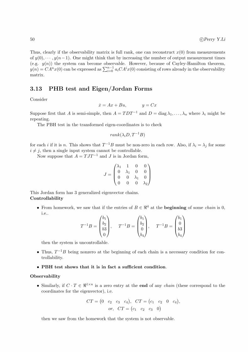
3.13 PHB test and Eigen/Jordan Forms
Considerx = Ax+Bu, y = Cx
Suppose first that A is semi-simple, then A = TDT−1 and D = diag λ1, . . . , λn where λi might berepeating.
The PBH test in the transformed eigen-coordinates is to check
rank(λiD,T−1B)
for each i if it is n. This shows that T−1B must be non-zero in each row. Also, if λi = λj for somei 6= j, then a single input system cannot be controllable.
Now suppose that A = TJT−1 and J is in Jordan form,
J =
λ1 1 0 00 λ1 0 00 0 λ1 00 0 0 λ2
This Jordan form has 3 generalized eigenvector chains.Controllability
• From homework, we saw that if the entries of B ∈ ℜ4 at the beginning of some chain is 0,i.e..
T−1B =
b1b2b30
, T−1B =
b1b20b4
, T−1B =
b10b3b4
then the system is uncontrollable.
• Thus, T−1B being nonzero at the beginning of each chain is a necessary condition for con-trollability.
• PBH test shows that it is in fact a sufficient condition.
Observability
• Similarly, if C · T ∈ ℜ1×n is a zero entry at the end of any chain (these correspond to thecoordinates for the eigenvector), i.e.
CT =(0 c2 c3 c4
), CT =
(c1 c2 0 c4
),
or, CT =(c1 c2 c3 0
)
then we saw from the homework that the system is not observable.
ME 8281:Advanced Control Systems, F01, F02, S06, S08 51
• Hence, CT having non-zero entries at the end of each chain is necessary for observability.
• PHB test shows that it is also sufficient.
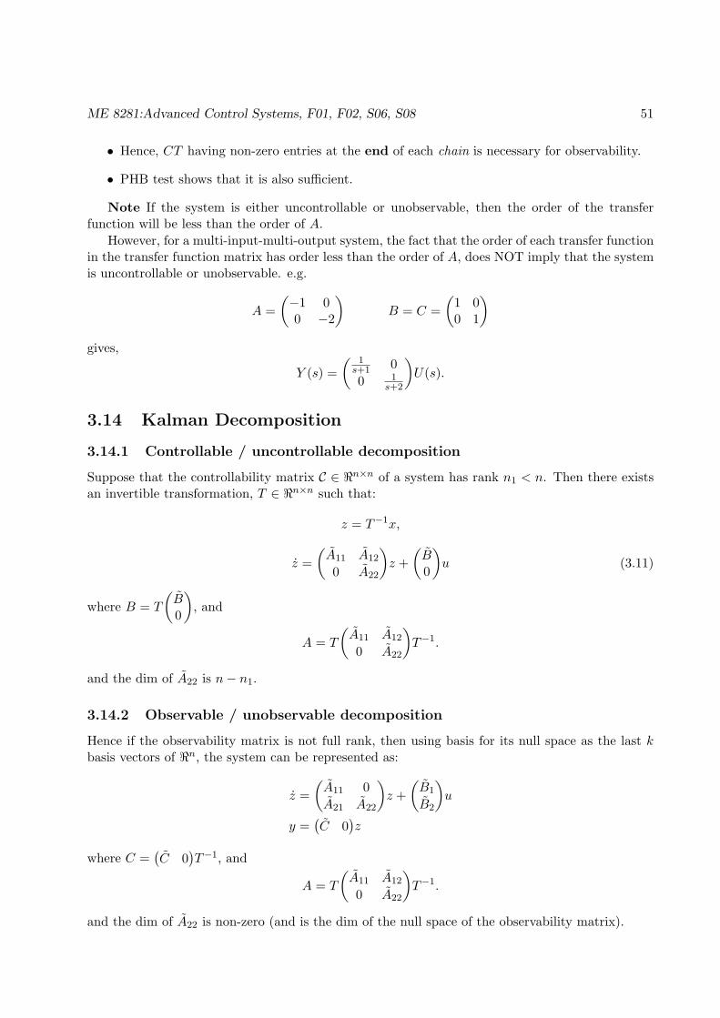
Note If the system is either uncontrollable or unobservable, then the order of the transferfunction will be less than the order of A.
However, for a multi-input-multi-output system, the fact that the order of each transfer functionin the transfer function matrix has order less than the order of A, does NOT imply that the systemis uncontrollable or unobservable. e.g.
A =
(−1 00 −2
)
B = C =
(1 00 1
)
gives,
Y (s) =
( 1s+1 0
0 1s+2
)
U(s).
3.14 Kalman Decomposition
3.14.1 Controllable / uncontrollable decomposition
Suppose that the controllability matrix C ∈ ℜn×n of a system has rank n1 < n. Then there existsan invertible transformation, T ∈ ℜn×n such that:
z = T−1x,
z =
(A11 A12
0 A22
)
z +
(B0
)
u (3.11)
where B = T
(B0
)
, and
A = T
(A11 A12
0 A22
)
T−1.
and the dim of A22 is n− n1.
3.14.2 Observable / unobservable decomposition
Hence if the observability matrix is not full rank, then using basis for its null space as the last kbasis vectors of ℜn, the system can be represented as:
z =
(A11 0
A21 A22
)
z +
(B1
B2
)
u
y =(C 0
)z
where C =(C 0
)T−1, and
A = T
(A11 A12
0 A22
)
T−1.
and the dim of A22 is non-zero (and is the dim of the null space of the observability matrix).
52 c©Perry Y.Li
3.14.3 Kalman decomposition
The Kalamn decomposition is just the combination of the observable/unobservable, and the con-trollable/uncontrollable decomposition.
Theorem 3.14.1 There exists a coordinate transformation z = T−1x ∈ ℜn such that
z =
A11 0 A13 0
A21 A22 A23 A24
0 0 A33 0
0 0 A43 A44
z +
B1
B2
00
u
y =(C1 0 C2 0
)z
Let T =(T1 T2 T3 T4
)(with compatible block sizes), then
• T2 → (C − O): T2 = basis for Range(C) ∩ Null(O).
• T1 → (C −O): T1 ∪ T2 = basis for Range(C)
• T4 → (C − O): T2 ∪ T4 = basis for Null(O).
• T3 → (C −O): T1 ∪ T2 ∪ T3 ∪ T4 = basis for ℜn.
Note: Only T2 is uniquely defined.
Proof: This is just combination of the obs/unobs and cont/uncont decomposition. ⋄
3.14.4 Stabilizability and Detectability
If the uncontrollable modes A33, A44 are stable (have eigenvalues on the Left Half Plane), then,system is called stabilizable.
• One can use feedback to make the system stable;
• Uncontrollable modes decay, so not an issue.
If the unobservable modes A22, A44 are stable (have eigenvalues on the Left Half Plane), then,system is called detectable.
• The states z2, z4 decay to 0
• Eventually, they will have no effect on the output
• State can be reconstructed by ignoring the unobservable states (eventually).
The PBH tests can be modified to check if the system is stabilizable or detectable, namely,check
rank(sI −A B
)rank
(sI −AC
)
for all s with non-negative real parts if they lose rank. Specifically, one needs to check only s whichare the unstable eigenvalues of A.
ME 8281:Advanced Control Systems, F01, F02, S06, S08 53
3.15 Realization
3.15.1 Degree of controllability / observability
Formal definitions for controllability and observability are black and white. In reality, some statesare very costly to control to, or have little effect on the outputs. They are therefore, effectivelyuncontrollable or unobservable.
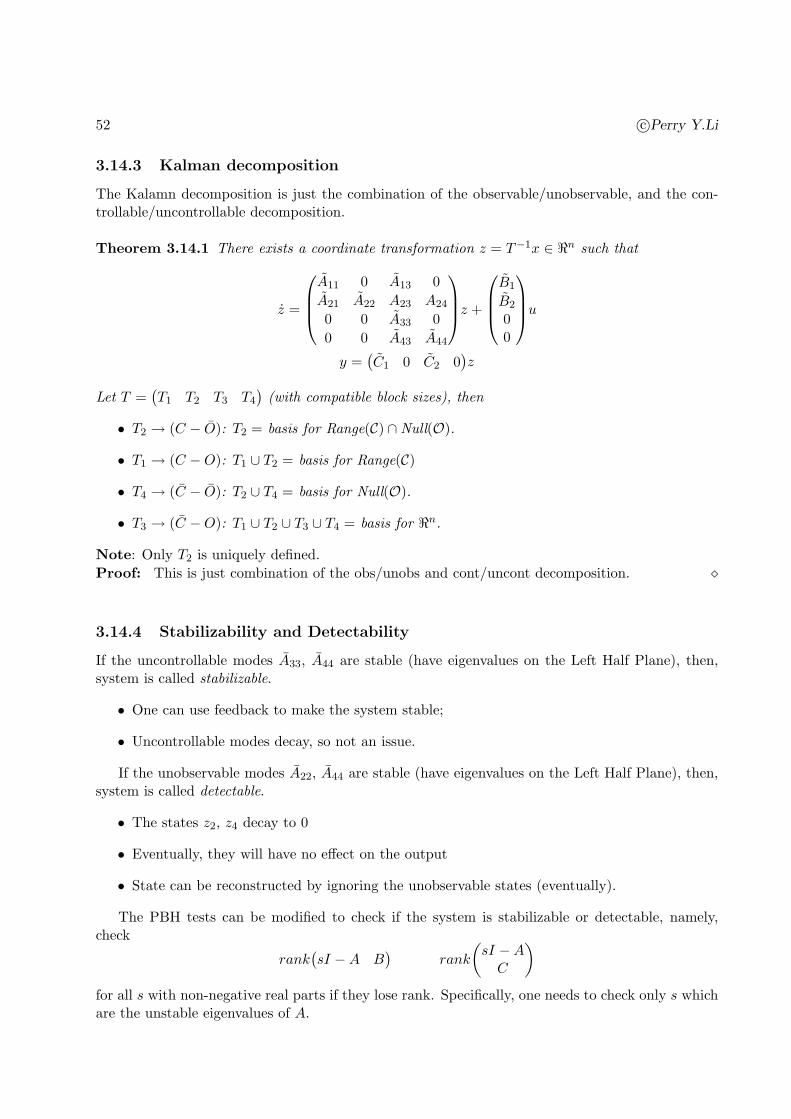
Degree of controllability and observability can be evaluated by the sizes of Wr and Wo withinfinite time horizon:
Wr(0,∞) = limT→∞
∫ T
0eA(T−τ)BBT eA
T (T−τ)dτ
=
∫ ∞
0eAtBBT eA
T tdt
Wo(0,∞) = limT→∞
∫ T
0eA
T τCTCeAτdτ
Notice that Wr satisfies differential equation:
d
dtWr(0, t) = AWr(0, t) +Wr(0, t)A
T +BBT
Thus, if all the eigenvalues of A have strictly negative real parts (i.e. A is stable), then, as T → ∞,
0 = AWr +WrAT +BBT
which is a set of linear equations in the entries of Wr, and can be solved effectively. The equationis called a Lyapunov equation. Matlab can solve for Wr using gram.
Similarly, if A is stable, as T → ∞, Wo satisfies the Lyapunov equation
0 = ATWo +WoA+ CTC
which can be solved using linear method (or using Matlab via gram).
Wr is related to the minimum norm control. To reach x(0) = x0 from x(−∞) = 0 in infinitetime,
u = LTr W
−1c x0
minu(·)J(u) = minu(·)
∫ 0
−∞uT (τ)u(τ)dτ = xT
0W−1c x0.
If state x0 is difficult to reach, then xT0W
−1c x0 is large meaning that x0 is practically uncontrollable.
Similarly, if the initial state is x(0) = x0, then, with u(τ) ≡ 0
∫ ∞
0yT (τ)y(τ)dτ = xT
0Wox0.
Thus, xT0Wox0 measures the effect of the initial condition on the output. If it is small, the effect of
x0 in the output y(·) is small, thus, it is hard to observe, or practically unobservable.
Generally, one can look at the smallest eigenvalues Wc and Wo, the span of the associatedeigenvectors will be difficult to control, or difficult to observe.
54 c©Perry Y.Li
3.15.2 Relation to Transfer Function
For the system
x = Ax+Bu
y = Cx+Du
The transfer function from U(s) → Y (s) is given by:
G(s) = C(sI −A)−1B +D
=Cadj(sI −A)B
det(sI −A)+D.
Note that transfer function is not affected by similarity transform.
From Kalman decomposition, it is obvious that
G(s) = C1(sI − A11)−1B1 +D
where A11, B1, C1 correspond to the controllable and observable component.
Poles
• they are values of s ∈ C s.t. G(s) becomes infinite.
• poles of G(s) are clearly the eigenvalues of A11.
Zeros
• For the SISO case, z ∈ C (complex numbers) is a zero if it makes G(z) = 0.
• Thus, zeros satisfy
Cadj(zI −A)B +Ddet(zI −A) = 0
assuming system is controllable and observable, otherwise, need to apply Kalman decompo-sition first.
• In the general MIMO case, a zero implies that there can be non-zero inputs U(s) that produceoutput Y (s) that is identically zero. Therefore, there exists X(z), U(z) such that:
zI −A X(z) = B U(z)
0 = C X(z) +D U(z)
This will be true if and only if at s = z
rank
(sI −A −B−C −D
)
is less than the normal rank of the matrix at other s.
We shall return to the multi-variable zeros when we discuss the effect of state feedback on the zeroof the system.
ME 8281:Advanced Control Systems, F01, F02, S06, S08 55
3.15.3 Pole-zero cancellation
Cascade system with input/output (u1, y2):
• System 1 with input/output (u1, y1) has a zero at α and a pole at β.
x1 = A1x1 +B1u1
y1 = C1x1
• System 2 with input/output (u2, y2)has a pole at α and a zero at β.
x2 = A2x2 +B2u2
y2 = C2x2
• Cascade interconnection: u2 = y1.
Then
1. The system pole at β is not observable from y2
2. The system pole at α is not controllable from u1.
Combined system:
A =
(A1 0B2C1 A2
)
; B =
(B1
0
)
; C =(0 C2
)
Consider x =
(x1
x2
)
.
• Use PBH test with λ = β.
βI −A1 0−B2C1 βI −A2
0 C2
(x1
x2
)
= 0???
• Let x1 be eigenvector associated with β for A1.
• Let x2 = (βI −A2)−1B2C2x1 (i.e. solve second row in PBH test).
• Then since
Cx = C2x2 = (C2(βI −A2)−1B2)C2x1
and β is a zero of system 2, PHB test shows that the mode β is not observable.
Similar for the case when α mode in system 2 not controllable by u.
These example shows that when cascading systems, it is important not to do unstable pole/zerocancellation.
56 c©Perry Y.Li
3.16 Balanced Realization
The objective is to reduce the number of states while minimizing effect on I/O response (transferfunction). This is especially useful when the state equations are obtained from distributed param-eters system, P.D.E. via finite elements methods, etc. which generate many states. If states areunobservable or uncontrollable, they can be removed. The issue at hand is if some states are lightlycontrollable while others are lightly observable. Do we cancel them?
In particular,
• Some states can be lightly controllable, but heavily observable.
• Some states can be lightly observable, but heavily controllable.
• Both contribute to significant component to input/output (transfer function) response.
Idea: Exhibit states so that they are simultaneously lightly (heavily) controllable and observ-able.
Consider a stable system:
x = Ax+Bu
y = Cx+Du
If A is stable, reachability and observability grammians can be computed by solving the Lya-punov equations:
0 = AWr +WrAT +BBT
0 = ATWo +WoA+ CTC
• If state x0 is difficult to reach, then xT0W
−1r x0 is large ⇒ practically uncontrollable.
• If xT0Wox0 is small, the signal of x0 in the output y(·) is small, thus, it is hard to observe ⇒
practically unobservable.
• Generally, one can look at the smallest eigenvalues Wr and Wo, the span of the associatedeigenvectors will be difficult to control, or difficult to observe.
Transformation of grammians: (beware of which side T goes !):
z = Tx
Minimum norm control should be invariant to coordinate transformation:
xT0W
−1r x0 = zTW−1
r,z z = xTT TW−1r,z Tx
ThereforeW−1
r = T TW−1r,z T ⇒Wr,z = T ·WrT
T .
Similarly, the energy in a state transmitted to output should be invariant:
xTWox = zWo,zz ⇒Wo,z = T−TWoT−1.
Theorem 3.16.1 (Balanced realization) If the linear time invariant system is controllable andobservable, then, there exists an invertible transformation T ∈ ℜn×n s.t. Wo,z = Wr,z.
ME 8281:Advanced Control Systems, F01, F02, S06, S08 57
The balanced realization algorithm:
1. Compute controllability and observability grammians:
>> Wr = gram(sys, ’c’);
>> Wo = gram(sys, ’o’)
2. Write Wo = RTR [One can use SVD]
>> [U,S,V]=svd(Wo);
>> R = sqrtm(S)*V’;
3. Diagonalize RWrRT [via SVD again]:
RWrRT = UΣ2UT ,
where UUT = I and Σ is diagonal.
>> [U1,S1,V1]=svd(R*Wr*R’);
>> Σ = sqrtm(S1’;
4. Take T = Σ− 1
2UTR
>> T = inv(sqrtm(Σ))*U1’*R;
5. This gives Wr,z = Wo,z = Σ.
>> Wr,z = T ∗Wr ∗ T′,
>> Wo,z = inv(T )′ ∗Wo ∗ inv(T )
Proof: Direct substitution!
• OnceWr,z andWo,z are diagonal, and equal, one can decide to eliminate states that correspondto the smallest few entries.
• Do not remove unstable states from the realization since these states need to be controlled(stabilized)
• It is also possible to maintain some D.C. performance.
Consider the system in the balanced realization form:
d
dt
(z1z2
)
=
(A11 A12
A21 A22
)(z1z2
)
+
(B1
B2
)
u
y = C1z2 + C2z2 +Du
where z1 ∈ ℜn1 and z2 ∈ ℜn2 , and n1 + n2 = n. Suppose that the z1 are associated with thesimultaneously lightly controllable and light observable mode.
The naive truncation approach is to remove z2 to form the reduced system:
z1 = A11z1 +B1u
y = C1z1 +Du
58 c©Perry Y.Li
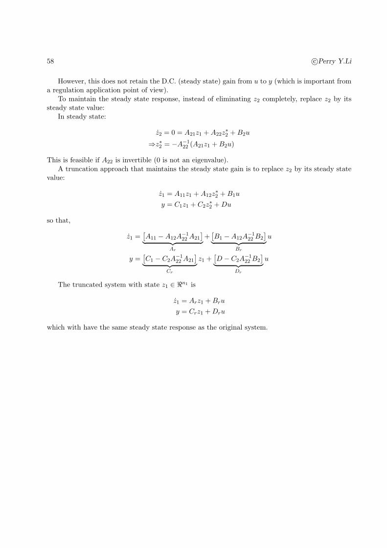
However, this does not retain the D.C. (steady state) gain from u to y (which is important froma regulation application point of view).
To maintain the steady state response, instead of eliminating z2 completely, replace z2 by itssteady state value:
In steady state:
z2 = 0 = A21z1 +A22z∗2 +B2u
⇒z∗2 = −A−122 (A21z1 +B2u)
This is feasible if A22 is invertible (0 is not an eigenvalue).A truncation approach that maintains the steady state gain is to replace z2 by its steady state
value:
z1 = A11z1 +A12z∗2 +B1u
y = C1z1 + C2z∗2 +Du
so that,
z1 =[A11 −A12A
−122 A21
]
︸ ︷︷ ︸
Ar
+[B1 −A12A
−122 B2
]
︸ ︷︷ ︸
Br
u
y =[C1 − C2A
−122 A21
]
︸ ︷︷ ︸
Cr
z1 +[D − C2A
−122 B2
]
︸ ︷︷ ︸
Dr
u
The truncated system with state z1 ∈ ℜn1 is
z1 = Arz1 +Bru
y = Crz1 +Dru
which with have the same steady state response as the original system.


![RESEARCH REPORT-2013-08-21 30–1 On the Controllability and ... · arXiv:1401.4335v1 [cs.SY] 17 Jan 2014 RESEARCH REPORT-2013-08-21 30–1 On the Controllability and Observability](https://img.pdfslide.us/doc/110x75/5fc991f91964ed6233533cb3/research-report-2013-08-21-30a1-on-the-controllability-and-arxiv14014335v1.jpg)