1

GPS-LiDAR Sensor Fusion Aided by 3D CityModels for UAVs

Akshay Shetty, Member, IEEE, and Grace Xingxin Gao, Senior Member, IEEE

Abstract—Outdoor positioning for Unmanned Aerial Vehicles(UAVs) commonly relies on GPS signals, which might be reflectedor blocked in urban areas. In such cases, additional on-boardsensors such as Light Detection and Ranging (LiDAR) aredesirable. To fuse GPS and LiDAR measurements, it is important,yet challenging, to accurately characterize the error covariance ofthe sensor measurements. In this paper, we propose a GPS-LiDARfusion technique with a novel method for modeling the LiDAR-based position error covariance as a function of the point cloudfeatures. We use the LiDAR point clouds to estimate incrementalmotion, and to estimate global pose by matching with a 3Dcity model. For GPS measurements, we use the 3D city modelto eliminate non-line-of-sight (NLOS) satellites and model themeasurement covariance based on the received signal-to-noise-ratio (SNR) values. Finally, we implement an Unscented KalmanFilter (UKF) to estimate the UAV’s global pose and analyze itsobservability. To validate our algorithm, we conduct outdoorexperiments and demonstrate a clear improvement in the UAV’sglobal pose estimation.

Keywords—Unmanned aerial vehicles (UAVs), light detectionand ranging (LiDAR), 3-dimensional (3D) city model, globalpositioning system (GPS), unscented kalman filter (UKF)

I. INTRODUCTION

Emerging applications in UAVs such as 3D modeling,filming, surveying, search and rescue, and delivering packages,involve flying in urban environments. In these scenarios,autonomously navigating a UAV has certain advantages suchas optimizing flight paths and sensing and avoiding collisions[1], [2]. However, to enable such autonomous control, we needa continuous and reliable source for the UAVs’ positioning. Inmost cases, GPS is primarily relied on for outdoor positioning.However, in an urban environment, GPS signals from the satel-lites are often blocked or reflected by surrounding structures,causing large errors in the position output [3].

Different GPS techniques [4] have been demonstrated toreduce the effect of multipath and NLOS signals on positioningerrors. These techniques include using coupled amplitude delaylock loops [5], using high-mask-angle antennas [6], and usingadaptive antenna arrays [7]. Furthermore, there has been a con-siderable amount of research into reducing positioning errorswith the aid of 3D city models. One of the methods includeschoosing candidate positions, predicting the measurements atthese positions using the 3D city model, and finally comparingthe predicted and received measurements to improve the pre-dicted position [8], [9]. In addition, other existing techniques

A. Shetty and G. X. Gao are with the Department of Aerospace Engineering,University of Illinois at Urbana-Champaign, Champaign IL, 61801 USA. E-mail: ashetty2@illinois.edu, gracegao@illinois.edu.

include shadow matching [10] and geometric modeling [11]or constraining [12] of the NLOS signals.

In cases when GPS is unreliable, additional on-board sensorssuch as LiDAR are commonly used to obtain the navigationsolution [13]. For simplicity, we refer to the LiDAR sensoras just LiDAR in this paper. An on-board LiDAR provides areal-time point cloud of the surroundings of the UAV. Thus,in a dense urban environment, LiDAR is able to detect alarge number of features from surrounding structures, such asbuildings.

Positioning based on LiDAR point clouds has been demon-strated primarily by applying different simultaneous localiza-tion and mapping (SLAM) algorithms [14]. In many cases,algorithms implement variants of Iterative Closest Point (ICP)[15] to register new point clouds [16], [17]. Other methodsnot dependent on ICP [18], [19], include point cloud matchingbased on polar coordinates of points [20] and tracking based onfeatures in a point cloud [21]. Implementation of some LiDAR-based SLAM algorithms [22]–[24] are available online.

Furthermore, there has been analysis on the error covarianceof position estimates from algorithms based on LiDAR pointclouds [25]–[27]. These methods have been demonstrated insimulations and practice, and include training kernels basedon likelihood optimization [28], [29], obtaining the covariancebased on the Fisher Information matrix [30], [31], and obtain-ing the covariance based on 2D scanned lines [32].

A. Related sensor fusion work

Different techniques to integrate LiDAR and GPS havebeen demonstrated to improve the overall navigation solution.The most straightforward way to integrate these sensors is toloosely-couple them, i.e. to directly use the position output.Prior work [33], [34] with LiDAR and GPS equipped UAVsdemonstrated such loosely-coupled architectures. However,in certain cases, a tightly-coupled sensor fusion architecturetends to work better than a loosely-coupled one. For ex-ample, position output from GPS receivers in urban areasgenerally contains errors or is unavailable. However, someof the intermediate psuedorange measurements are possiblyaccurate and can aid in positioning [35], [36]. Tightly-coupledarchitectures with GPS and a 2D laser scanner [37], [38] havebeen demonstrated to provide an accurate navigation solutionin challenging environments. Another application of a tightly-coupled structure, to eliminate NLOS satellites by detectingthe skyline from omnidirectional camera images [39], [40],has also shown an improvement in urban positioning.

2

B. Our approach

The main contribution of this paper is a GPS-LiDAR fu-sion technique with a novel method for efficiently modelingthe error covariance in position measurements derived fromLiDAR point clouds. Figure 1 shows the different componentsinvolved in the sensor fusion.

We use the LiDAR point clouds in two ways: to estimateincremental motion by matching consecutive point clouds; and,to estimate global pose by matching with a 3D city model. Weuse ICP for matching the point clouds in both cases.

For the LiDAR-based position estimates, we proceed tobuild the error covariance model depending on the surroundingpoint cloud. First, we extract surface and edge feature pointsfrom the point cloud. We then model the position errorcovariance based on these individual feature points. Finally,we combine all the individual covariance matrices to modelthe overall position error covariance ellipsoid.

For the GPS measurement model, we use the pseudor-ange measurements from a stationary reference receiver andan on-board GPS receiver to obtain a vector of double-difference measurements. Using the double-difference mea-surements eliminates clock bias and atmospheric error terms,hence reducing the number of unknown variables. We use theglobal position estimate from the LiDAR - 3D city matching toconstruct LOS vectors to all the detected satellites. We then usethe 3D city model to detect NLOS satellites, and consequentlyrefine the double-difference measurement vector. We create acovariance matrix for the GPS double-difference measurementvector based on SNR of the individual pseudorange measure-ments.

We implement an UKF to integrate all LiDAR and GPSmeasurements. Additionally, we incorporate orientation, ori-entation rate and acceleration measurements from an on-boardinertial measurement unit (IMU). We perform an observabilitytest [41] for the filter, based on Lie derivatives. Finally, wetest the filter on an urban dataset to show an improvement inthe navigation solution.

Fig. 1: Overview of sensor fusion architecture

C. Outline of Paper

In this paper we present a more extensive version of ourwork in [42], including detailed analysis and additional exper-imental results. Section II introduces the point cloud matchingalgorithm that we use for odometry based on consecutivepoint clouds. Section III introduces the LiDAR - 3D citymodel matching algorithm. It first discusses the steps takento build the 3D city model. It then analyzes the performanceof using ICP for matching in urban environments. Section IVfocuses on building the error covariance model for positionestimates obtained from the LiDAR. It models the covarianceellipsoid as a function of the distribution of surface and edgefeatures in the point cloud. Section V focuses on creating theGPS measurement vector and it’s covariance. It introducesthe model for the received GPS pseudorange measurements,and the steps taken to create a vector of double-differencemeasurements. Section VI presents the UKF structure to in-tegrate the measurements from GPS and LiDAR, describedin the previous sections. It then presents an observabilityanalysis of the filter structure. Next, it elaborates details ofthe experimental setup and evaluates the filter performance onan urban dataset. Finally, Section VII concludes the paper.

II. LIDAR-BASED ODOMETRY

ICP is commonly used for registering three-dimensionalpoint clouds. It takes a reference point cloud q, an inputpoint cloud p, and estimates the rotation matrix R and thetranslation vector T between the two point clouds. There hasbeen extensive literature introducing different variants of thealgorithm [15]. These generally consist of three primary steps:• Matching: This step involves matching each point pi in

the input point cloud, to a point qi in the reference pointcloud. The most common method is to find the nearestneighbors of each point in the input point cloud. For ourapplication, a kDtree performs best since the two pointclouds are relatively close to each other [43].

• Defining error metric: This step defines the error metricfor the point pairs. We choose the point-to-point metric,which is generally more robust to difficult geometry thanother metrics such as point-to-plane [15]. The total errorbetween the two point clouds is defined as follows:

E =

N∑i=1

‖R · pi + T− qi‖ , (1)

where N is the number of points in the input point cloudp.

• Minimization: The last step of the algorithm is theminimization of the error metric w.r.t. the rotation matrixR and the translation vector T between the two pointclouds.

We use ICP to estimate the incremental motion of theLiDAR between consecutive point clouds. The previous Li-DAR point cloud is used as the reference q and the currentLiDAR point cloud is used as the input p. Figure 2 shows ourimplementation [44] of ICP to estimate the LiDAR odometry.

3

(a) Before ICP matching (b) After ICP matching

Fig. 2: The input to ICP is a reference point cloud q and aninput point cloud p as shown in (a). The algorithm calculatesthe rotation matrix R and the translation vector T such thatthe error metric E is minimized. (b) shows the reference pointcloud q and the transformed input point cloud R · p + T.

III. MATCHING LIDAR AND 3D CITY MODEL

A. Generating 3D city modelWe generate our 3D city model using data from two

sources: Illinois Geospatial Data Clearinghouse [45] and Open-StreetMap (OSM) [46]. The Illinois Geospatial Data werecollected by a fixed wing aircraft flying at an altitude of1700 meters, equipped with a LiDAR system including adifferential GPS unit and an inertial measurement system toprovide superior global accuracy. Since the data were collectedfrom a relatively high altitude, it primarily contains adequatedetails for the ground surface and the building rooftops. Inorder to complete the 3D city model, we need additionalinformation for the sides of buildings. We use OpenStreetMap(OSM) to obtain this information. OSM is a freely available,crowd-sourced map of the world, which allows users to obtaininformation such as building footprints and heights [47]. Figure3 shows a section of the 3D city model for Champaign County.

B. On-board LiDAR - 3D city model matchingIn order to estimate the global pose of the LiDAR, we match

the on-board LiDAR point cloud with the 3D city model usingICP described in section II. We implement the following steps:

(a) (b)

Fig. 3: Section of the point cloud for Champaign Countydataset. (a) shows the 3D city model using just the IllinoisGeospatial Data. (b) shows the model after incorporatingbuilding information from OpenStreetMap.

• Use the position output from on-board GPS receiver asan initial guess. If position output is unavailable, usethe position estimate from the previous iteration as aninitial guess. For orientation, use the estimate from theprevious iteration. Thus, we obtain an initial pose guessx0L.

• Project the on-board LiDAR point cloud pL to the samespace as the 3D city model qcity using x0

L.• Implement ICP, to obtain the rotation RL and translation

TL between the two point clouds. Use this output toobtain an estimate for the global pose xL.

Figure 4 shows the results of implementation of the abovemethod. While navigating in urban areas, the GPS receiverposition output used for the initial pose guess x0

L might containlarge errors in certain directions. This might cause ICP toconverge to a local minimum, depending on features in thepoint cloud pL generated by the on-board LiDAR.

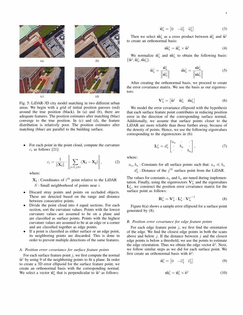
To evaluate how our LiDAR - 3D city model matchingalgorithm performs in such challenging cases, we test it intwo different urban areas as shown in Figure 5. We begin byselecting a grid of initial position guesses up to 20 metersaway from the true position. With an adequate distribution offeatures, ICP is able to correctly match the two point cloudsand provide an accurate position estimate after matching. Incontrast, when there’s an urban scenario with a relatively poordistribution of features, ICP is unable to estimate the positionaccurately.

IV. MODELING LIDAR POSITION ERROR COVARIANCE

Based on the observations made in section III, we modelthe LiDAR position error covariance as a function of thesurrounding features. In urban environments, we typicallyobserve structured objects such as buildings. Hence, we focusprimarily on surface and edge features in the point cloud. Weextract these feature points based on the curvature at eachpoint, as described in [21]. The algorithm can be summarizedin the following steps:

(a) Before matching step (b) After matching step

Fig. 4: Global pose estimation with the aid of a 3D city model.(a) shows the initial position guess x0

L (red) and the on-boardLiDAR point cloud pL projected on the same space as the 3Dcity model qcity . (b) shows the updated global position xL(green) after the ICP step. We observe an improvement in theglobal position, as the LiDAR point cloud matches with the3D city model.

4

(a) (b)

(c) (d)

Fig. 5: LiDAR-3D city model matching in two different urbanareas. We begin with a grid of initial position guesses (red)around the true position (black). In (a) and (b), there areadequate features. The position estimates after matching (blue)converge to the true position. In (c) and (d), the featuredistribution is relatively poor. The position estimates aftermatching (blue) are parallel to the building surface.

• For each point in the point cloud, compute the curvatureci as follows [21]:

ci =1

‖Xi‖·

∥∥∥∥∥∥∑

jεS,j 6=i

(Xi −Xj)

∥∥∥∥∥∥ , (2)

where:

Xi : Coordinates of ith point relative to the LiDARS : Small neighborhood of points near i.

• Discard stray points and points on occluded objects.These are detected based on the range and distancebetween consecutive points.

• Divide the point cloud into 4 equal sections. For eachsection, sort the curvature values. Points with the lowestcurvature values are assumed to be on a plane andare classified as surface points. Points with the highestcurvature values are assumed to be at an edge or a cornerand are classified together as edge points.

• If a point is classified as either surface or an edge point,its neighboring points are discarded. This is done inorder to prevent multiple detections of the same features.

A. Position error covariance for surface feature pointsFor each surface feature point j, we first compute the normal

uj by using 9 of the neighboring points to fit a plane. In orderto create a 3D error ellipsoid for the surface feature point, wecreate an orthonormal basis with the corresponding normal.We select a vector ~nju that is perpendicular to uj as follows:

~nju =[0 −uj3 uj2

](3)

Then we select ~mju as a cross product between ~nju and uj

to create an orthonormal basis:

~mju = ~nju × uj (4)

We normalize ~nju and ~mju to obtain the following basis:

{uj , nju, mju}.

nju =~nju∥∥∥~nju∥∥∥ mj

u =~mju∥∥∥ ~mju

∥∥∥ (5)

After creating the orthonormal basis, we proceed to createthe error covariance matrix. We use the basis as our eigenvec-tors:

Vju =

[uj nju mj

u

](6)

We model the error covariance ellipsoid with the hypothesisthat each surface feature point contributes in reducing positionerror in the direction of the corresponding surface normal.Additionally, we assume that surface points closer to theLiDAR are more reliable than those further away, because ofthe density of points. Hence, we use the following eigenvaluescorresponding to the eigenvectors in (6):

Lju = dju

[au · ·· bu ·· · bu

], (7)

where:

au, bu : Constants for all surface points such that: au � bu

dju : Distance of the jth surface point from the LiDAR.

The values for constants au and bu are tuned during implemen-tation. Finally, using the eigenvectors Vj

u and the eigenvaluesLju, we construct the position error covariance matrix for thesurface point as follows:

Rju = Vj

u · Lju ·Vju

−1(8)

Figure 6(a) shows a sample error ellipsoid for a surface pointgenerated by (8).

B. Position error covariance for edge feature pointsFor each edge feature point j, we first find the orientation

of the edge. We find the closest edge points in both the scansabove and below j. If the distance between j and the closestedge points is below a threshold, we use the points to estimatethe edge orientation. Thus we obtain the edge vector ej . Next,we follow similar steps as we did for each surface point. Wefirst create an orthonormal basis with ej :

~nje =[0 −ej3 ej2

](9)

~mje = ~nje × ej (10)

5

(a) (b)

Fig. 6: Position error covariance ellipsoid for surface and edgefeature points. (a) shows the covariance ellipsoid Rj

u con-tributed by the jth surface point. uj represents the correspond-ing surface normal; and nju and mj

u complete orthonormalbasis. (b) shows the covariance ellipsoid Rj

e contributed by thejth edge point. ej represents the corresponding edge vector;and nje and mj

e complete orthonormal basis.

After normalizing ~nje and ~mje as done in (5), we obtain the

required basis {ej , nje, mje}, which we use as the eigenvectors:

Vje =

[ej nje mj

e

](11)

We model the error covariance ellipsoid with the hypothesisthat each edge feature point helps in reducing position errorin the directions perpendicular to the edge vector. A verticaledge, for example, would help in reducing horizontal positionerror. Additionally, we assume that edge points closer to theLiDAR are more reliable than those further away, because ofthe density of points. Hence, we use the following eigenvaluescorresponding to the eigenvectors in (11):

Lje = dje

[ae · ·· be ·· · be

], (12)

where:

ae, be : Constants for all edge points such that: ae � be

dje : Distance of the jth edge point from the LiDAR.

The values for constants ae and be are tuned during implemen-tation. Finally, using the eigenvectors Vj

e and the eigenvaluesLje, we construct the position error covariance matrix for theedge point as follows:

Rje = Vj

e · Lje ·Vje

−1(13)

Figure 6(b) shows a sample error ellipsoid for an edge pointgenerated by (13).

C. Combining error ellipsoidsIn order to obtain the overall position error covariance, we

combine the error covariance matrices for all the individualsurface and edge feature points. The combined covariancematrix can be obtained as [48]:

RL =

nu∑j=1

Rju

−1+

ne∑j=1

Rje

−1

−1 , (14)

where Rje and Rj

u are the covariance matrices from individ-ual surface (8) and edge (13) feature points respectively; nuand ne are the number of surface and edge feature points inthe point cloud.

Figure 7 shows the resulting position error covariance el-lipsoids RL for two point clouds in urban environments. Inthe horizontal plane, the covariance ellipsoid is larger in thedirection parallel to the building sides. In the vertical direction,the size of the covariance ellipsoid remains constrained due topoints detected on the ground.

V. GPS MEASUREMENT MODEL

To create the GPS measurement model, we use the pseudor-ange measurements. The measurement between a GPS receiveru and the kth satellite can be modelled as [49]:

ρku = rku + c[δtu − δtk] + Ikρu + T kρu + εkρu , (15)

where:

rku : True range between receiver u and kth satellitec : Speed of light

δtu : Clock bias for receiver uδtk : Clock bias for kth satelliteIkρu : Ionospheric error

T kρu : Tropospheric error

εkρu : Noise in pseudorange measurement.

In order to eliminate certain error terms, we use double-difference pseudorange measurements, which are calculatedby differencing the pseudorange measurements between two

Fig. 7: Overall position error ellipsoids RL, for two pointclouds generated by the on-board LiDAR in an urban envi-ronment.

6

satellites and between two receivers. The double differencepseudorange measurements between two satellites k and l, andbetween two GPS receivers u and r can be represented as:

ρk·lur = (ρku − ρkr )− (ρlu − ρlr)≈ (rkur + cδtur + εkρur

)− (rlur + cδtur + εlρur)

= (rkur − rlur) + εk·lρur, (16)

where for short baselines between the two receivers, theionospheric and tropospheric errors can be assumed to benegligible. Furthermore, the baseline between the two receiverscan be assumed to be significantly smaller than the distancebetween the receivers and the satellites. Thus, the range termrkur in (16) can be approximated as:

rkur = rku − rkr ≈ −1kr · xur, (17)

where, xur is the baseline between the two receivers; and1kr is a unit vector from the receiver r to the satellite k asshown in Figure 8. Using (17), the above expression for thedouble difference pseudorange measurement can be expressedas follows:

ρk·lur ≈ −(1kr − 1lr) · xur + εk·lρur(18)

A. NLOS satellites eliminationBefore proceeding to create the vector of GPS double

difference pseudorange measurements, we check if any of thesatellites detected by the receiver are non-line-of-sight signals.We use the 3D city model described in section III-A to detectthe NLOS satellites. We use the position output generated bythe LiDAR-3D city model matching, as described in sectionIII, to locate the receiver on the 3D city model. Next, we drawLOS vectors from the receiver to every satellite detected bythe receiver and eliminate satellites whose corresponding LOSvectors intersect the 3D city model. Fig. 9 shows the aboveimplementation in an urban scenario.

Fig. 8: Geometry of single-difference measurements. Here xuand xr are the positions of the user and reference receivers inthe Earth Centered Earth Fixed (ECEF) frame [49]. The base-line between these receivers xur, is assumed to be significantlysmaller than the ranges to the satellites rku and rkr .

B. GPS measurement vector and covarianceAfter eliminating the NLOS satellites, we select satellites

that are visible to both the user and the reference receiversto create the GPS measurement vector and its covariance.The vector of double-difference pseudorange measurementsbetween the receivers can be represented as:

ρDDur =

ρ1·Kurρ2·Kur

...ρ(K−1)·Kur

= ADD ·

ρ1uρ2u...ρKuρ1rρ2r...ρKr

, (19)

where ADD relates the individual pseudorange measure-ments to the double-difference measurements based on (16).Once we have the vector of GPS measurements, we proceedto model its covariance. We assume that the individual pseu-dorange measurements are independent, and that the variancefor each measurement is a function of the corresponding SNR(C/N0)

ku in dB, where k refers to the kth satellites and u refers

to the user receiver [50]. We use the following covariancematrices for the user and the reference receivers respectively:

Rρu = diag(10−(C/N0)1u

10 , 10−(C/N0)2u

10 , · · · , 10−(C/N0)Ku

10 ) (20)

Rρr = diag(10−(C/N0)1r

10 , 10−(C/N0)2r

10 , · · · , 10−(C/N0)Kr

10 ) (21)

To obtain the covariance matrix for the double-differencemeasurements, we propagate the above covariance matrices asfollows:

Fig. 9: Elimination of NLOS satellite signals. The receiverposition (black) is projected on the 3D city model. LOS vectorsare drawn to all detected satellites: SV3, SV14, SV16, SV22,SV23, SV26, SV31. The LOS vectors to satellites SV23 andSV31 intersect (red) the 3D city model and are eliminated fromfurther calculations.

7

RρDDur

= ADD ·[Rρu

Rρr

]·ADD

T (22)

VI. GPS-LIDAR INTEGRATION

A. Unscented kalman filter structure

In addition to using a LiDAR and a GPS receiver, we use anIMU on-board the UAV. Figure 10 shows the different framesof reference used in the filter. The state vector consists of thefollowing states:

xT =[pug

T , vugT , qug

T , bωT , ba

T , qigT], (23)

where pug , vug , and qug are the position, velocity and theorientation respectively of the UAV in the local GPS frame;bω and ba are the IMU gyroscope and accelerometer biases;qig is the orientation offset between the local GPS and IMUframes.

For the prediction step of the filter, we use a constantvelocity model. Additionally, we include the angular velocityωm, and acceleration am measurements from the IMU inthe prediction step [51], instead of the relatively expensivecorrection step. Thus, the prediction step can be written as:

pug

vug

qug

bω

ba

qig

︸ ︷︷ ︸

x

=

vug

−RT(qu

g )ba−g0.5Ξ(qu

g )bω

000

︸ ︷︷ ︸

f0(x)

+

00

0.5Ξ(qug )

000

︸ ︷︷ ︸

f1(x)

ωm

︸︷︷︸u1

+

0

RT(qu

g )

0000

︸ ︷︷ ︸

f2(x)

am

︸︷︷︸u2

, (24)

where R(qug )

represents the rotation between the UAV frameand the local GPS frame; Ξ(qu

g )expresses the time rate of

change of (qug ) [52]. (24) can be re-written compactly as:

x = f0(x) + f1(x)u1 + f2(x)u2, (25)

with x, f0, f1, f2, u1 and u2 as marked in (24).For the correction step, we use pose information from the

LiDAR, orientation information from the IMU and positioninformation from the GPS receiver. From the LiDAR we usepose information from two sources: one from the LiDARodometry described in section II, and the other from theLiDAR - 3D city model matching described in section III. TheLiDAR odometry measurements relate to the state variables asfollows:

h1 = R(qug )(pug − pug ) (26)

h2 = R(qug )

RT(qu

g ), (27)

where pug and qug refer to the previous filter estimate of positionand orientation of the UAV in the local GPS frame. The LiDAR- 3D city model matching measurements directly relate to thestate variables:

h3 = pug (28)

h4 = qug . (29)

Fig. 10: Frames of reference. The local GPS frame (blue)refers to the local North-East-Down (NED) frame centered atposition where UAV begins operation. The IMU frame (red)is slightly offset the local GPS frame due to biases in themagnetometers. The UAV frame (green) is fixed to the bodyof the UAV.

The orientation measurement from the IMU is with respect toframe that is offset with respect to the local GPS frame. Thus,it relates to the state variables as follows:

h5 = qig ⊗ qug . (30)

For measurements from the GPS receiver, we use the double-difference measurements ρDD

ur from (19). These measurementscan be related to the state variables as follows:

h6 = G1 · ((pug )ECEF − pref )

h7 = G2 · ((pug )ECEF − pref )

...h(K−1)+5 = GK−1 · ((pug )ECEF − pref ),

(31)

where K is the number of satellites; (pug )ECEF and pref arethe positions of the UAV and the reference receiver in theECEF frame [49]; G is a function of the unit vectors from thereference receiver to the satellites being used in the double-difference calculation, as shown in (18).

The measurements h1 and h2 are in the LiDAR frame. Thus,for the covariance of h1, we use RL from (14). The measure-ments h3 and h4 are from LiDAR - 3D city model matching,which are in the local GPS frame. Thus, for covariance of h3,we rotate RL to the local GPS frame as follows [53]:

RGPSL = RT

(qug )·RL ·R(qu

g )(32)

For the orientation measurements h2, h4 and h5, we usea fixed diagonal matrix. For the GPS double-difference mea-surements, we use the covariance matrix RρDD

urfrom (22).

B. Non-linear observability analysis of filter

To ensure that all the state variables are observable, wecheck the observability of our system using Lie derivatives

8

[51], [52], [54]. The zeroth order Lie derivative of a functionh, is calculated as:

L0h(x) = h(x) (33)

Further derivatives of h, with respect to a function f , iscalculated recursively as:

Lkfh(x) =∂(Lk−1f h(x))

∂xf(x) (34)

We use (33) and (34) on the measurements (26)-(31) toobtain the necessary Lie derivatives for the observation matrix:

O=

∇L0h1

∇L0h2

∇L0h3

∇L0h4

∇L0h5

∇L0h6

∇L0h7

∇L0h8

∇L1f0

h1

∇L1f0

h2

∇L2f0f0

h1

=

R(qug ) 0 0 0 0 0

0 0 a[2,3]3×4 0 0 0

I3×3 0 0 0 0 00 0 I4×4 0 0 0

0 0 a[5,3]4×4 0 0 a

[5,6]4×4

a[6,1]1×3 0 0 0 0 0

a[7,1]1×3 0 0 0 0 0

a[8,1]1×3 0 0 0 0 0

0 R(qug ) 0 0 0 0

0 0 a[10,3]3×4 a

[10,4]3×3 0 0

0 0 a[11,3]3×4 0 a

[11,5]3×3 0

(35)

In the above matrix, we can see that ∇L0h1, ∇L0h3 or∇L0h6,∇L0h7,∇L0h8 together, account for the observabilityof the position states pug . The observability of the velocityvug , is accounted for by ∇L1

f0h1. Additionally, ∇L1

f0h3 or

∇L1f0h6, ∇L1

f0h7, ∇L1

f0h8 together, would also make vug ob-

servable, but have not been included in (35) to keep the matrixconcise. ∇L0h2 or ∇L0h4, account for the observability ofthe orientation qug . The biases bω and ba are observable dueto ∇L1

f0h2 and ∇L2

f0f0h1. Finally, the orientation offset qig

is observable due to ∇L0h5.For practical applications, there might be cases where the

3D city model is not available, thus making measurementsh3 and h4 unavailable. Furthermore, while navigating throughdense urban environments, the GPS measurements h6, h7, h8might be unavailable. In these cases, theoretically the filterstates would still be observable with the measurements h1, h2

and h5. However, h3, h4, h6, h7 and h8 act as corrections toprevent the state variables from drifting.

C. Implementation and experimental resultsWe use the iBQR UAV designed and built by our research

group for data collection. The UAV has an arm length of 0.6m, and a payload capacity of 2 kg. We use a Velodyne VLP-16Puck Lite LiDAR, a ublox LEA-6T GPS receiver connectedto a Maxtena antenna, and an Xsens Mti-30 IMU. We use anAscTec MasterMind as the on-board computer, to log the datafrom all these sensors. We limit the range of the LiDAR to15 meters, in order to evaluate the LiDAR-based algorithmsin certain under-constrained situations. For our reference GPSreceiver, we use a Trimble NetR9 receiver within a kilometerof our data collection sites, which allows us to proceed withthe short baseline assumptions made in section V.

Fig. 11: Experimental setup for data collection. Our custom-made iBQR UAV mounted with a LiDAR, a GPS receiver andantennas, an IMU, and an on-board computer.

To initialize the filter, we assume that the UAV beginsoperation in an open-sky environment with accurate and re-liable GPS signals. We keep the UAV stationary and averagethe GPS receiver position output for the first few secondsto create the local GPS frame, which is used throughout thefilter implementation. We initialize all state variables as zero,except for qig . We keep the UAV facing approximately Northand average the first few seconds of IMU measurements toinitialize qig . Finally, we initialize the state covariance matrixas an identity matrix.

We implement the UKF on an urban dataset collected onour campus of University of Illinois at Urbana-Champaign.For our trajectory, we begin at the South-West corner of theHydrosystems Building, head North and keep moving alongthe building till we reach our starting position again.

Before implementing the filter, we see how the differentmeasurement sources perform for our dataset. As shown inFigure 12, the GPS measurements and the GPS position outputcontain large errors, due to the presence of nearby urban struc-tures. Here we stack all the double difference measurementsfrom (18) and compute the unweighted least square estimateof the baseline between the UAV and the reference receiver.

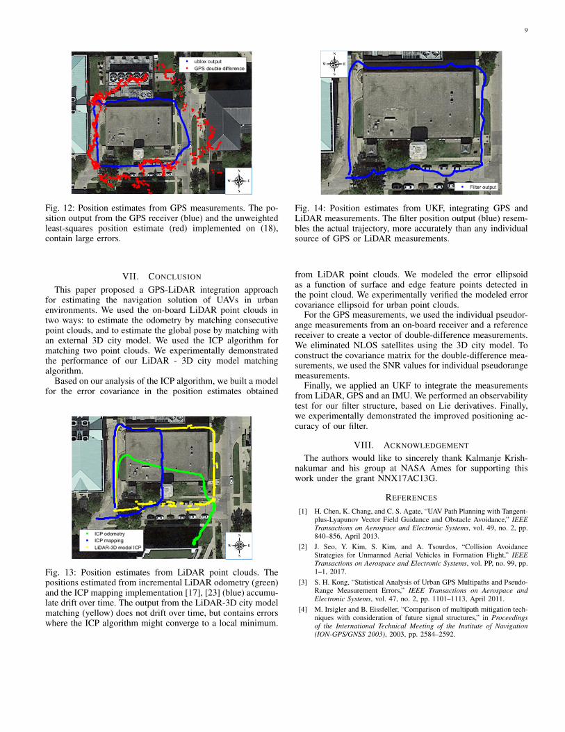
For the LiDAR measurements we check the output fromsimple ICP registration method as explained in section II andthe LiDAR - 3D city model matching algorithm describedin section III. Furthermore, we implement an ICP mappingalgorithm [17], [23] to check the performance of existingICP-based methods on the dataset. As shown in Figure 13,the ICP registration method and the ICP mapping algorithmaccumulate drift over the course of the trajectory. The LiDAR- 3D city model matching algorithm does not drift over time,since the 3D city model is globally referenced. However,the position outputs still contain errors in situations wherethe LiDAR does not detect enough number of points or thematching algorithm converges to a local minimum.

Figure 14 shows the output of the filter for the sametrajectory. The filter output estimates the actual path muchmore accurately than the individual measurement sources bythemselves.

9

Fig. 12: Position estimates from GPS measurements. The po-sition output from the GPS receiver (blue) and the unweightedleast-squares position estimate (red) implemented on (18),contain large errors.

VII. CONCLUSION

This paper proposed a GPS-LiDAR integration approachfor estimating the navigation solution of UAVs in urbanenvironments. We used the on-board LiDAR point clouds intwo ways: to estimate the odometry by matching consecutivepoint clouds, and to estimate the global pose by matching withan external 3D city model. We used the ICP algorithm formatching two point clouds. We experimentally demonstratedthe performance of our LiDAR - 3D city model matchingalgorithm.

Based on our analysis of the ICP algorithm, we built a modelfor the error covariance in the position estimates obtained

Fig. 13: Position estimates from LiDAR point clouds. Thepositions estimated from incremental LiDAR odometry (green)and the ICP mapping implementation [17], [23] (blue) accumu-late drift over time. The output from the LiDAR-3D city modelmatching (yellow) does not drift over time, but contains errorswhere the ICP algorithm might converge to a local minimum.

Fig. 14: Position estimates from UKF, integrating GPS andLiDAR measurements. The filter position output (blue) resem-bles the actual trajectory, more accurately than any individualsource of GPS or LiDAR measurements.

from LiDAR point clouds. We modeled the error ellipsoidas a function of surface and edge feature points detected inthe point cloud. We experimentally verified the modeled errorcovariance ellipsoid for urban point clouds.

For the GPS measurements, we used the individual pseudor-ange measurements from an on-board receiver and a referencereceiver to create a vector of double-difference measurements.We eliminated NLOS satellites using the 3D city model. Toconstruct the covariance matrix for the double-difference mea-surements, we used the SNR values for individual pseudorangemeasurements.

Finally, we applied an UKF to integrate the measurementsfrom LiDAR, GPS and an IMU. We performed an observabilitytest for our filter structure, based on Lie derivatives. Finally,we experimentally demonstrated the improved positioning ac-curacy of our filter.

VIII. ACKNOWLEDGEMENT

The authors would like to sincerely thank Kalmanje Krish-nakumar and his group at NASA Ames for supporting thiswork under the grant NNX17AC13G.

REFERENCES

[1] H. Chen, K. Chang, and C. S. Agate, “UAV Path Planning with Tangent-plus-Lyapunov Vector Field Guidance and Obstacle Avoidance,” IEEETransactions on Aerospace and Electronic Systems, vol. 49, no. 2, pp.840–856, April 2013.

[2] J. Seo, Y. Kim, S. Kim, and A. Tsourdos, “Collision AvoidanceStrategies for Unmanned Aerial Vehicles in Formation Flight,” IEEETransactions on Aerospace and Electronic Systems, vol. PP, no. 99, pp.1–1, 2017.

[3] S. H. Kong, “Statistical Analysis of Urban GPS Multipaths and Pseudo-Range Measurement Errors,” IEEE Transactions on Aerospace andElectronic Systems, vol. 47, no. 2, pp. 1101–1113, April 2011.

[4] M. Irsigler and B. Eissfeller, “Comparison of multipath mitigation tech-niques with consideration of future signal structures,” in Proceedingsof the International Technical Meeting of the Institute of Navigation(ION-GPS/GNSS 2003), 2003, pp. 2584–2592.

10

[5] X. Chen, F. Dovis, S. Peng, and Y. Morton, “Comparative Studies ofGPS Multipath Mitigation Methods Performance,” IEEE Transactionson Aerospace and Electronic Systems, vol. 49, no. 3, pp. 1555–1568,July 2013.

[6] L. Heng, T. Walter, P. Enge, and G. X. Gao, “GNSS Multipath andJamming Mitigation Using High-Mask-Angle Antennas and MultipleConstellations,” IEEE Transactions on Intelligent Transportation Sys-tems, vol. 16, no. 2, pp. 741–750, April 2015.

[7] M. T. Brenneman, Y. T. Morton, and Q. Zhou, “GPS MultipathDetection with ANOVA for Adaptive Arrays,” IEEE Transactions onAerospace and Electronic Systems, vol. 46, no. 3, pp. 1171–1184, July2010.

[8] S. Miura, L. T. Hsu, F. Chen, and S. Kamijo, “GPS Error CorrectionWith Pseudorange Evaluation Using Three-Dimensional Maps,” IEEETransactions on Intelligent Transportation Systems, vol. 16, no. 6, pp.3104–3115, Dec 2015.

[9] P. D. Groves, Z. Jiang, L. Wang, and M. K. Ziebart, “Intelligenturban positioning using multi-constellation GNSS with 3D mappingand NLOS signal detection,” in Proceedings of the 25th InternationalTechnical Meeting of The Satellite Division of the Institute of Navigation(ION GNSS+ 2012), Nashville, TN, USA, 2012, pp. 458–472.

[10] P. D. Groves, “Shadow matching: A new GNSS positioning techniquefor urban canyons,” Journal of Navigation, vol. 64, no. 03, pp. 417–430,2011.

[11] A. Bourdeau, M. Sahmoudi, and J. Tourneret, “Tight integration ofGNSS and a 3D city model for robust positioning in urban canyons,” inProceedings of the 25th International Technical Meeting of The SatelliteDivision of the Institute of Navigation (ION GNSS+ 2012), Nashville,TN, USA, 2012, pp. 1263 – 1269.

[12] V. Drevelle and P. Bonnifait, “iGPS: Global Positioning in UrbanCanyons with Road Surface Maps,” IEEE Intelligent TransportationSystems Magazine, vol. 4, no. 3, pp. 6–18, Fall 2012.

[13] H. Zhao, M. Chiba, R. Shibasaki, X. Shao, J. Cui, and H. Zha, “ALaser-Scanner-Based Approach Toward Driving Safety and Traffic DataCollection,” IEEE Transactions on Intelligent Transportation Systems,vol. 10, no. 3, pp. 534–546, Sept 2009.

[14] C. Cadena, L. Carlone, H. Carrillo, Y. Latif, D. Scaramuzza, J. Neira,I. Reid, and J. J. Leonard, “Past, present, and future of simultaneouslocalization and mapping: toward the robust-perception age,” IEEETransactions on Robotics, vol. 32, no. 6, pp. 1309–1332, 2016.

[15] S. Rusinkiewicz and M. Levoy, “Efficient variants of the ICP algorithm,”in Proceedings Third International Conference on 3-D Digital Imagingand Modeling, 2001, pp. 145–152.

[16] F. Moosmann and C. Stiller, “Velodyne SLAM,” in 2011 IEEE Intelli-gent Vehicles Symposium (IV), June 2011, pp. 393–398.

[17] F. Pomerleau, F. Colas, R. Siegwart, and S. Magnenat, “Comparing ICPvariants on real-world data sets,” Autonomous Robots, vol. 34, no. 3,pp. 133–148, 2013.

[18] M. Kaess, A. Ranganathan, and F. Dellaert, “iSAM: IncrementalSmoothing and Mapping,” IEEE Transactions on Robotics, vol. 24,no. 6, pp. 1365–1378, Dec 2008.

[19] S. Kohlbrecher, O. von Stryk, J. Meyer, and U. Klingauf, “A flexible andscalable SLAM system with full 3D motion estimation,” in 2011 IEEEInternational Symposium on Safety, Security, and Rescue Robotics, Nov2011, pp. 155–160.

[20] A. Diosi and L. Kleeman, “Laser scan matching in polar coordinateswith application to SLAM,” in 2005 IEEE/RSJ International Conferenceon Intelligent Robots and Systems, Aug 2005, pp. 3317–3322.

[21] J. Zhang and S. Singh, “LOAM: Lidar Odometry and Mapping in Real-time,” in Robotics: Science and Systems, vol. 2, 2014.

[22] Google, “Cartographer,” 2016. [Online]. Available:https://github.com/googlecartographer.

[23] F. Pomerleau and S. Magnenat, “ethzasl icp mapping,”May 2016, [ROS software package]. [Online]. Available:http://wiki.ros.org/ethzasl icp mapping.

[24] M. Quigley, K. Conley, B. P. Gerkey, J. Faust, T. Foote, J. Leibs,R. Wheeler, and A. Y. Ng, “ROS: an open-source Robot OperatingSystem,” in ICRA Workshop on Open Source Software, 2009.

[25] O. Bengtsson and A. J. Baerveldt, “Robot localization based on scan-matchingestimating the covariance matrix for the IDC algorithm,”Robotics and Autonomous Systems, vol. 44, no. 1, pp. 29–40, 2003.

[26] M. Brenna, “Scan matching, covariance estimation and SLAM: modelsand solutions for the scanSLAM algorithm,” Artificial Intelligence andRobotics Laboratory Politecnico di Milano, 2009.

[27] S. Liu, M. M. Atia, Y. Gao, and A. Noureldin, “Adaptive covarianceestimation method for LiDAR-aided multi-sensor integrated navigationsystems,” Micromachines, vol. 6, no. 2, pp. 196–215, 2015.

[28] A. Bachrach, S. Prentice, R. He, and N. Roy, “RANGE–Robust au-tonomous navigation in GPS-denied environments,” Journal of FieldRobotics, vol. 28, no. 5, pp. 644–666, 2011.

[29] W. Vega-Brown and N. Roy, “CELLO-EM: Adaptive sensor modelswithout ground truth,” in 2013 IEEE/RSJ International Conference onIntelligent Robots and Systems, Nov 2013, pp. 1907–1914.

[30] A. Censi, “An accurate closed-form estimate of ICP’s covariance,”in Proceedings 2007 IEEE International Conference on Robotics andAutomation, April 2007, pp. 3167–3172.

[31] A. Censi, “On achievable accuracy for range-finder localization,” inProceedings 2007 IEEE International Conference on Robotics andAutomation, April 2007, pp. 4170–4175.

[32] A. Soloviev, D. Bates, and F. Graas, “Tight coupling of laser scannerand inertial measurements for a fully autonomous relative navigationsolution,” Navigation, vol. 54, no. 3, pp. 189–205, 2007.

[33] S. Hening, C. A. Ippolito, K. S. Krishnakumar, V. Stepanyan, andM. Teodorescu, “3D LiDAR SLAM Integration with GPS/INS for UAVsin Urban GPS-Degraded Environments,” in AIAA Information Systems-AIAA Infotech@ Aerospace, 2017, pp. 0448–0457.

[34] Y. Lin, J. Hyyppa, and A. Jaakkola, “Mini-UAV-Borne LIDAR for Fine-Scale Mapping,” IEEE Geoscience and Remote Sensing Letters, vol. 8,no. 3, pp. 426–430, May 2011.

[35] I. Miller and M. Campbell, “Sensitivity Analysis of a Tightly-CoupledGPS/INS System for Autonomous Navigation,” IEEE Transactions onAerospace and Electronic Systems, vol. 48, no. 2, pp. 1115–1135, April2012.

[36] A. Soloviev, “Tight Coupling of GPS and INS for Urban Navigation,”IEEE Transactions on Aerospace and Electronic Systems, vol. 46, no. 4,pp. 1731–1746, October 2010.

[37] M. Joerger and B. Pervan, “Measurement-level integration of carrier-phase GPS and laser-scanner for outdoor ground vehicle navigation,”Journal of Dynamic Systems, Measurement, and Control, vol. 131, no. 2,pp. 021 004–021 014, 2009.

[38] A. Soloviev, “Tight coupling of GPS, laser scanner, and inertial mea-surements for navigation in urban environments,” in 2008 IEEE/IONPosition, Location and Navigation Symposium, May 2008, pp. 511–525.

[39] T. Suzuki, M. Kitamura, Y. Amano, and T. Hashizume, “High-accuracyGPS and GLONASS positioning by multipath mitigation using omnidi-rectional infrared camera,” in 2011 IEEE International Conference onRobotics and Automation, May 2011, pp. 311–316.

[40] J. i. Meguro, T. Murata, J. i. Takiguchi, Y. Amano, and T. Hashizume,“GPS Multipath Mitigation for Urban Area Using OmnidirectionalInfrared Camera,” IEEE Transactions on Intelligent TransportationSystems, vol. 10, no. 1, pp. 22–30, March 2009.

[41] M. Bryson and S. Sukkarieh, “Observability analysis and active controlfor airborne SLAM,” IEEE Transactions on Aerospace and ElectronicSystems, vol. 44, no. 1, pp. 261–280, January 2008.

[42] A. Shetty and G. X. Gao, “Covariance Estimation for GPS-LiDARSensor Fusion for UAVs,” in Proceedings of the 30th InternationalTechnical Meeting of The Satellite Division of the Institute of Navigation(ION GNSS+ 2017), Portland, OR, USA, 2017.

11

[43] H. M. Kjer and J. Wilm, “Evaluation of surface registration algorithmsfor PET motion correction,” B.S. thesis, Technical University of Den-mark, DTU, 2010.

[44] J. Wilm, “Iterative Closest Point,” January 2013. [Online]. Avail-able: https://www.mathworks.com/matlabcentral/fileexchange/27804-iterative-closest-point.

[45] “Illinois Geospatial Data Clearinghouse,” 2015. [Online]. Available:https://clearinghouse.isgs.illinois.edu/.

[46] M. Haklay and P. Weber, “OpenStreetMap: User-Generated StreetMaps,” IEEE Pervasive Computing, vol. 7, no. 4, pp. 12–18, Oct 2008.

[47] “OpenStreetMap.” [Online]. Available: www.openstreetmap.org.[48] I. Pokrajac, P. Okiljevic, and V. Desimir, “Fusion of multiple estimation

of emitter positions,” Scientific Technical Review, vol. 62, no. 3-4, pp.55–61, 2012.

[49] P. Misra and P. Enge, “Global Positioning System: Signals, Mea-surements and Performance Second Edition,” Massachusetts: Ganga-Jamuna Press, 2006.

[50] J. Collins and R. Langley, “Possible weighting schemes for GPS carrierphase observations in the presence of multipath,” Final contract reportfor the US Army Corps of Engineers Topographic Engineering Center,No. DAAH04-96-C-0086/TCN, vol. 98151, 1999.

[51] S. M. Weiss, “Vision based navigation for micro helicopters,” Ph.D.dissertation, Citeseer, 2012.

[52] J. Kelly and G. S. Sukhatme, “Visual-inertial sensor fusion: localiza-tion, mapping and sensor-to-sensor self-calibration,” The InternationalJournal of Robotics Research, vol. 30, no. 1, pp. 56–79, 2011.

[53] V. Spruyt, “A geometric interpretation of the covariance matrix,” 2014.[Online]. Available: http://www.visiondummy.com/2014/04/geometric-interpretation-covariance-matrix/.

[54] R. Hermann and A. Krener, “Nonlinear controllability and observabil-ity,” IEEE Transactions on Automatic Control, vol. 22, no. 5, pp. 728–740, Oct 1977.

Akshay Shetty received the B.Tech. degree inaerospace engineering from Indian Institue of Tech-nology, Bombay, India in 2014. He received the M.S.degree in aerospace engineering from Universityof Illinois at Urbana-Champaign in 2017. He hasworked as an Intern at NASA Ames Research Center,California during summer 2016 and summer 2017.He is currently pursuing the PhD degree at Univer-sity of Illinois at Urbana-Champaign. His researchinterests include robotics and control.

Grace Xingxin Gao received the B.S. degree inmechanical engineering and the M.S. degree in elec-trical engineering from Tsinghua University, Bei-jing, China in 2001 and 2003. She received thePhD degree in electrical engineering from StanfordUniversity in 2008. From 2008 to 2012, she was aresearch associate at Stanford University. Since 2012,she has been with University of Illinois at Urbana-Champaign, where she is presently an assistant pro-fessor in the Aerospace Engineering Department.Her research interests are systems, signals, control,

and robotics.