1

Efficient Available Transfer Capability Analysis Using Linear

Methods

November 7, 2000

PSERC Internet Seminar

Jamie Weber

weber@powerworld.com

Power Systems Software Developer

PowerWorld Corporation

Urbana, IL

http://powerworld.com

2

What is Available Transfer Capability (ATC)?

• Some of you may be familiar with the terms– Total Transfer Capability (TTC)

– Capacity Benefit Margin (CBM)

– Transmission Reliability Margin (TRM)

– “Existing Transmission Commitments”

– Etc…

• Then ATC is defined as– ATC = TTC – CBM – TRM – “Existing TC”

• This talk will not cover these terms. – We will really be covering the calculation of “TTC”, but

let’s not get caught up with the nomenclature.

3

Available Transfer Capability

• In broad terms, let’s define ATC as– The maximum amount of additional MW transfer possible

between two parts of a power system• Additional means that existing transfers are considered part of the

“base case” and are not included in the ATC number

• Typically these two parts are control areas– Can really be any group of power injections.

• What does Maximum mean?– No overloads should occur in the system as the transfer is

increased

– No overloads should occur in the system during contingencies as the transfer is increased.

4

Computational Problem?

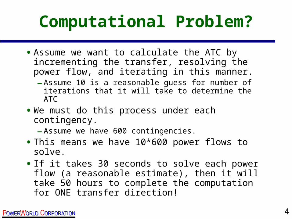
• Assume we want to calculate the ATC by incrementing the transfer, resolving the power flow, and iterating in this manner.– Assume 10 is a reasonable guess for number of

iterations that it will take to determine the ATC

• We must do this process under each contingency.– Assume we have 600 contingencies.

• This means we have 10*600 power flows to solve.

• If it takes 30 seconds to solve each power flow (a reasonable estimate), then it will take 50 hours to complete the computation for ONE transfer direction!

5

Why is ATC Important?

• It’s the point where power system reliability meets electricity market efficiency.

• ATC can have a huge impact on market outcomes and system reliability, so the results of ATC are of great interest to all involved.

6

Example: The Bonneville Power Administration (BPA)

• BPA operates a HUGE capacity of hydro-electric generating stations– Example: The Grand Coulee Dam has a capacity of

6,765 MW (it’s one dam!)

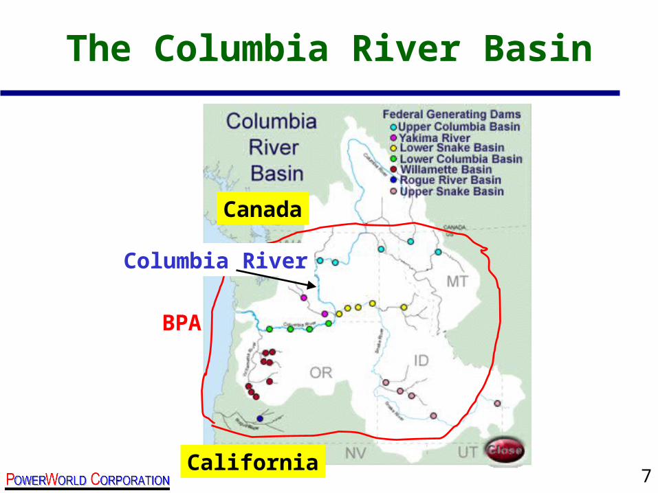
• Most of BPA’s capacity is along the Columbia River which starts in Canada

• As a result, how Canada utilizes its part of the Columbia River has a huge impact on the ability of BPA to utilize its Hydro Units along the river

7

The Columbia River Basin

BPA

Canada

California

Columbia River

8

Columbia River Basin

• The United States and Canada operate the Columbia River under a Treaty Agreement

• To state the Treaty in highly over-simplified terms– Canada has built and operates Columbia River Dams to

the benefit of the United States (i.e. BPA’s hydro units)

– BPA must make all attempts to give Canada access to markets in the US (i.e. California)

• This means BPA is always trying to ship power across its system between California and Canada.

• Huge amount of money is at stake– During the first 3 months of 2000, BC Hydro sold over

$1 billion in electricity to California!

9

Linear Analysis Techniques in PowerWorld Simulator

An overview of the underlying mathematics of the power flow

Explanation of where the linearized analysis techniques come from

10

AC Power Flow Equations

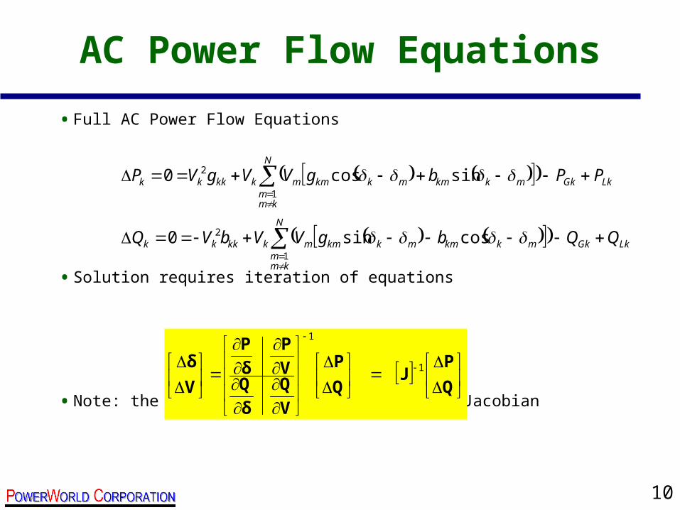
• Full AC Power Flow Equations

• Solution requires iteration of equations

• Note: the large matrix (J) is called the Jacobian

LkGk

N

kmm

mkkmmkkmmkkkkk

LkGk

N

kmm

mkkmmkkmmkkkkk

QQbgVVbVQ

PPbgVVgVP

1

2

1

2

cossin0

sincos0

Q

PJ

Q

P

V

Q

δ

QV

P

δ

P

V

δ 1

1

11

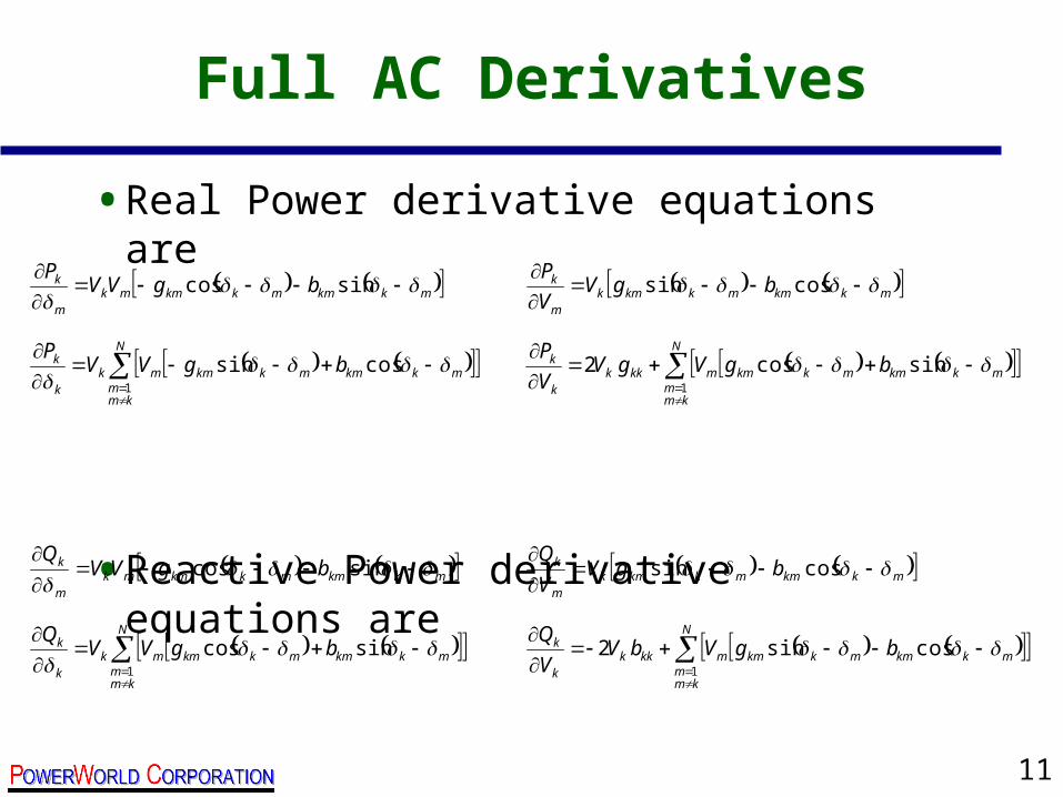
Full AC Derivatives

• Real Power derivative equations are

• Reactive Power derivative equations are

N

kmm

mkkmmkkmmkkkk

k bgVgVV

P

1

sincos2

N

kmm

mkkmmkkmmkk

k bgVVP

1

cossin

N

kmm

mkkmmkkmmkkkk

k bgVbVV

Q

1

cossin2

N

kmm

mkkmmkkmmkk

k bgVVQ

1

sincos

mkkmmkkmkm

k bgVV

P

cossin mkkmmkkmmkm

k bgVVP

sincos

mkkmmkkmkm

k bgVV

Q

cossin mkkmmkkmmkm

k bgVVQ

sincos

12

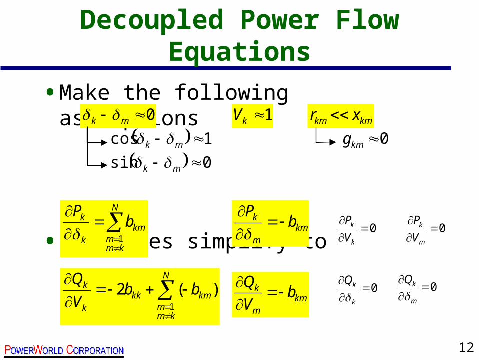
Decoupled Power Flow Equations

• Make the following assumptions

• Derivates simplify to

1kV kmkm xr 0 mk

0sin mk 1cos mk

0

k

k

V

P

N

kmm

kmk

k bP

1 0

m

k

V

Pkm

m

k bP

N

kmm

kmkkk

k bbV

Q

1

)(2 0

k

kQ

kmm

k bV

Q

0

m

kQ

0kmg

13

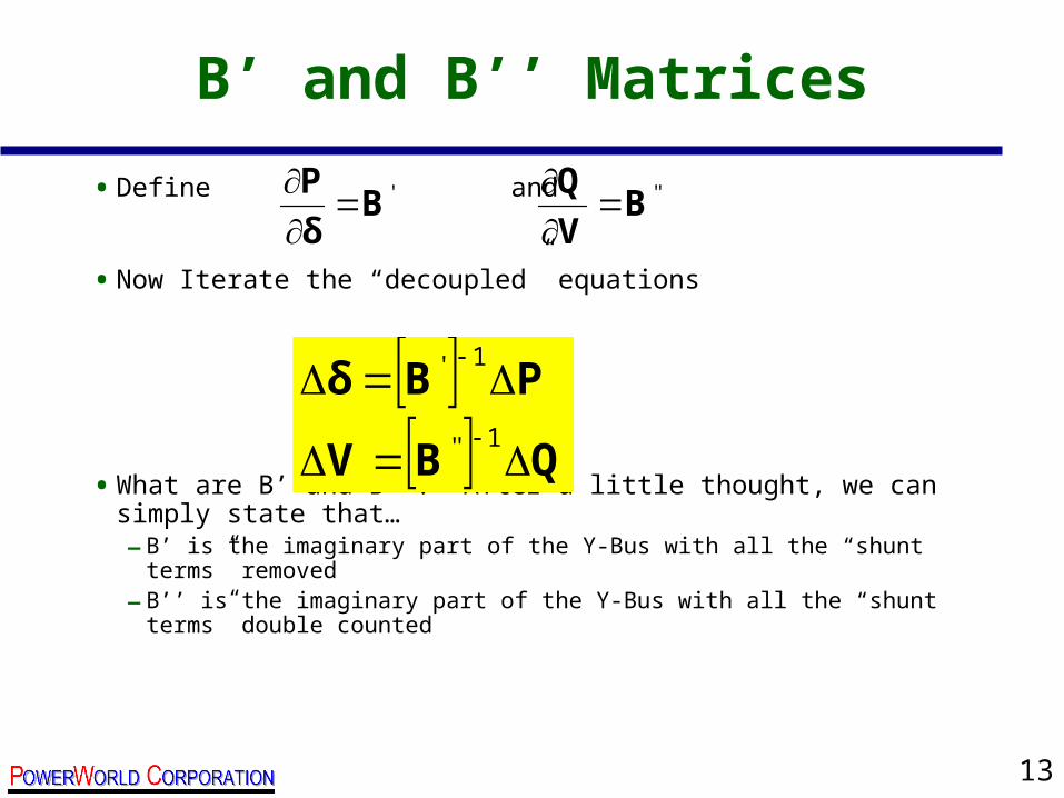
B’ and B’’ Matrices

• Define and

• Now Iterate the “decoupled” equations

• What are B’ and B’’? After a little thought, we can simply state that…– B’ is the imaginary part of the Y-Bus with all the “shunt terms” removed

– B’’ is the imaginary part of the Y-Bus with all the “shunt terms” double counted

'Bδ

P

''B

V

Q

QBV

PBδ

1''

1'

14

“DC Power Flow”

• The “DC Power Flow” equations are simply the real part of the decoupled power flow equations–Voltages and reactive power are ignored

–Only angles and real power are solved for by iterating

PBδ 1'

15

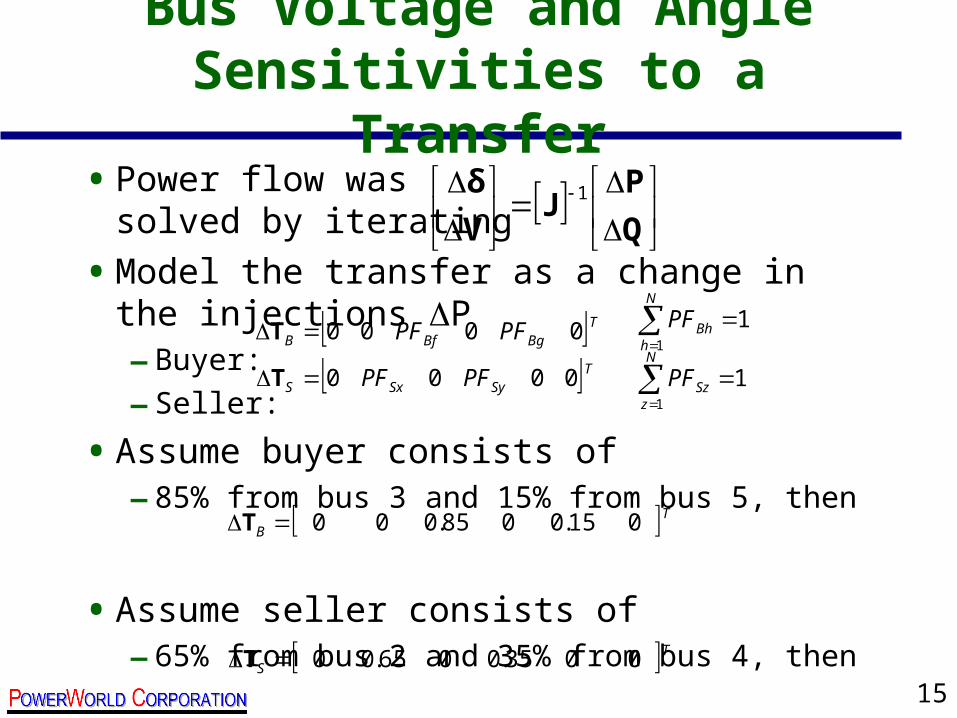
Bus Voltage and Angle Sensitivities to a Transfer

• Power flow was solved by iterating

• Model the transfer as a change in the injections P– Buyer:

– Seller:

• Assume buyer consists of– 85% from bus 3 and 15% from bus 5, then

• Assume seller consists of – 65% from bus 2 and 35% from bus 4, then

Q

PJ

V

δ 1

TSySxS PFPF 0000T 1

1

N

zSzPF

TBgBfB PFPF 0000T 1

1

N

hBhPF

TB 015.0085.000T

TS 0035.0065.00T

16

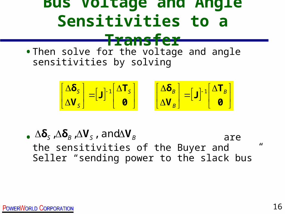
Bus Voltage and Angle Sensitivities to a Transfer

• Then solve for the voltage and angle sensitivities by solving

• are the sensitivities of the Buyer and Seller “sending power to the slack bus”

0

TJ

V

δ S

S

S 1

0

TJ

V

δ B

B

B 1

BSBS VVδδ and ,,,

17

What about Losses?

• If we assume the total sensitivity to the transfer is the seller minus the buyer sensitivity, then

• Implicitly, this assumes that ALL the change in losses shows up at the slack bus.

• PowerWorld Simulator assigns the change to the BUYER instead by defining

• Then

BS δδδ BS VVV

slack power to sendingbuyer for generation busslack in Change

slack power to sendingseller for generation busslack in Change

B

S

Slack

Slackk

B

B

S

S kV

δ

V

δ

V

δ

18

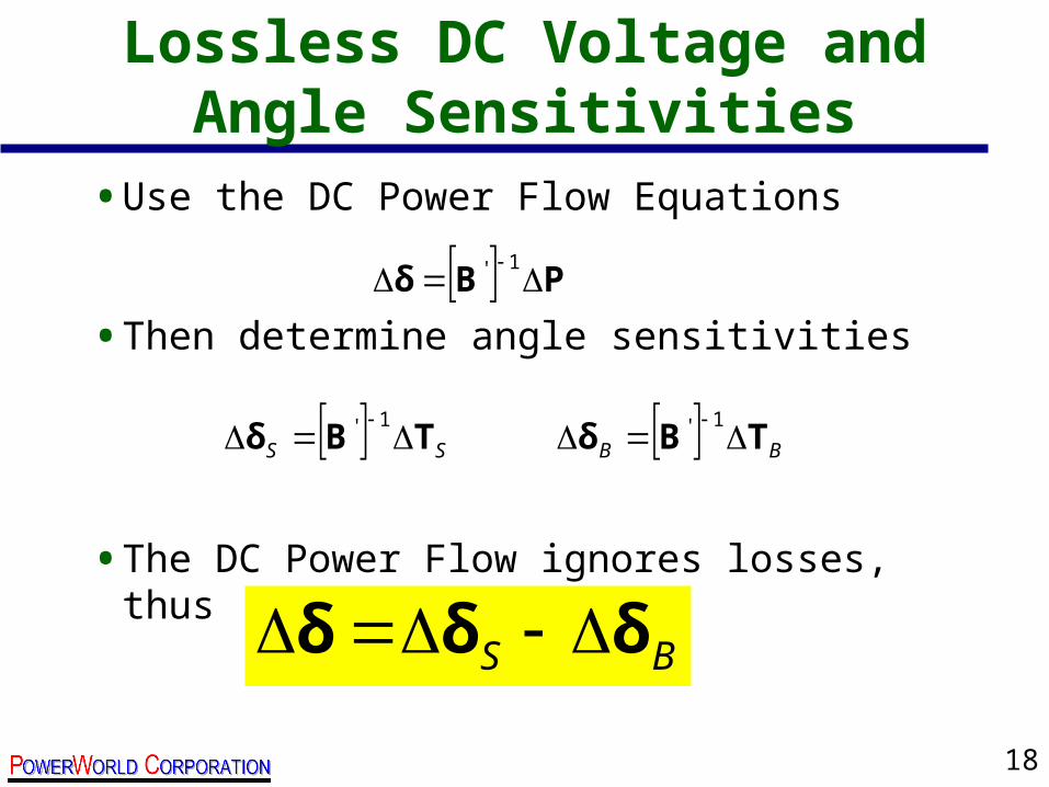
Lossless DC Voltage and Angle Sensitivities

• Use the DC Power Flow Equations

• Then determine angle sensitivities

• The DC Power Flow ignores losses, thus

PBδ 1'

SS TBδ 1' BB TBδ

1'

BS δδδ

19

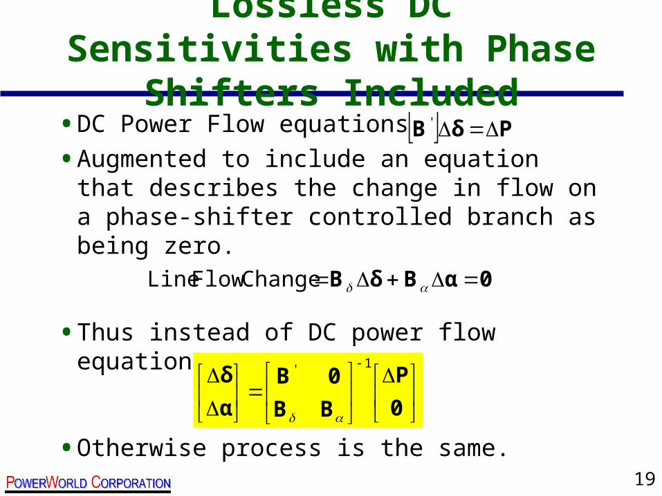
Lossless DC Sensitivities with Phase Shifters Included

• DC Power Flow equations

• Augmented to include an equation that describes the change in flow on a phase-shifter controlled branch as being zero.

• Thus instead of DC power flow equations we use

• Otherwise process is the same.

PδB '

0αBδB Change Flow Line

0

P

BB

0B

α

δ1'

20

Why Include Phase Shifters?

• Phase Shifters are often on lower voltage paths (230 kV or less) with relatively small limits

• They are put there in order to manage the flow on a path that would otherwise commonly see overloads

• Without including them in the sensitivity calculation, they constantly show up as “overloaded” when using Linear ATC tools

1 0 0 0 M W

6 5 3 M W

1 9 9 M V R

6 5 3 M W

1 0 5 M V R1 0 5 M V R

1 7 7 M V R

1 9 M V R

6 7 0 M W

3 0 M W

101 MVR1155 MW

769 MW 26 MVR

2 6 M V R

7 6 9 M W

2 M V R 2 6 M V R 5 M W7 6 9 M W

9 5 M W- 4 5 M V R

15 MVR114 MVR 30 MW540 MW

M I D P O I N T

M I D P O I N T

A D E L A I D E

I D A H O - N V

C O Y O T E C R

H U M B O L D T

V A L M Y

V A L M Y G 2

O L I N D A & 2R O U N D M T

O L I N D A & 1

R O U N D & 2 R O U N D & 4

R O U N D & 1

C A P T J A C K

M A L I N

M E R I D I N P

D I X O N V & 1

C A P T J A & 1 G R I Z Z L & 7

M A L I N & 1

C A P T J A & 2

G R I Z Z L & 6

D I X O N V L E

A L V E Y & 2

G R I Z Z L & 5C A P T J A & 3

M A L I N & 2

S U M M E R L

C A P T J A & 4

P O N D R O & 2

P O N D R O & 1

G R I Z Z L & 3

P O N D R O S A

C A P T J A & 5

G R I Z Z L Y

B O A R D F

B O A R D F

B U C K L E & 1G R I Z Z L & 1

G R I Z Z L & 2

B U C K L E Y

B U C K L E & 2

S L A T T

J O H N D A Y

J O H N D A Y

J O H N D & 1

A S H E & 2

O S T R N D E R

P E A R L

K E E L E R

S A N T I A M

M A R I O N

L A N E

A L V E Y

A L V E Y & 1

P A U L

C E N T R G 1

S A T S O P

O L Y M P I A

A S H E & 1

S A C J A W E A

S A C J W A T

A S H E 2L O W M O N

L O W M O NA S H E

H A N F O R D

V A N T A G E

S C H U L T Z

C O U L E E & 2

C O U L E E & 4

S I C K L E R

C O V I N G T 2

C O V I N G T N

R A V E R

T A C O M A

E C H O L A K E

C H I E F & 1

M O N R O E

C U S T E R W

W A H 3 6 0

R O S 3 6 0

I N G 5 0 0

M D N 5 0 0

D M R 5 0 0

G A R R I S & 1

G A R R I S & 3

G A R R I S & 4

G A R R I S & 2

T A F T

H O T S P R

D W O R 1

D W O R 2

D W O R S H A K

D W O R 3

H A T W A I

L O W G R A N

L O W G R A N

L I T G O O S

L I T G O O S

C O U L E E & 3

C O U L E E & 1

C O U L E E

C O U L E E 2 0C O U L E E 1 9

C H I E F J O

C H I E F J 5

S E L 5 0 0

C B K 5 0 0

B O R A H

A D E L T A P

B U R N S & 1

B U R N S

G R I Z Z L & 4

B U R N S & 2

R O U N D B U

C O Y O T E

B E L L B & 1B E L L B P A

A L L S T O N

B I G E D D Y

C E L I L O

H A N F O R & 1

M A P L E V L

M C L O U G L N

T R O U T D A L

R D M T 1 M

S N O H O M S 3

S N O H O M S 4

C O Y O D 1

C H I E F & 1

C H I E F & 2

C H I E F J 3

C H I E F J 4

M A P L E & 1

R O C K Y R H

N L Y 2 3 0

M C N A R Y

230 kV Phase Shifter

115 kV Phase Shifter

115 kV Phase Shifter

California

Canada

BPA

Weak LowVoltage TieTo Canada

21

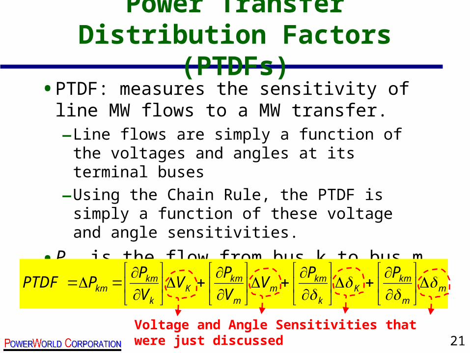
Power Transfer Distribution Factors (PTDFs)

• PTDF: measures the sensitivity of line MW flows to a MW transfer. –Line flows are simply a function of the voltages

and angles at its terminal buses

–Using the Chain Rule, the PTDF is simply a function of these voltage and angle sensitivities.

• Pkm is the flow from bus k to bus m

mm

kmK

k

kmm

m

kmK

k

kmkm

PPV

V

PV

V

PPPTDF

Voltage and Angle Sensitivities that were just discussed

22

Pkm Derivative Calculations

• Full AC equations

• Lossless DC Approximations yield

P

VV g V g bkm

kk kk m km k m km k m2 cos sin

P

VV g bkm

mk km k m km k mcos sin

PV V g bkm

kk m km k m km k m

sin cos

PV V g bkm

mk m km k m km k m

sin cos

0

k

km

V

P0

m

km

V

P

kmk

km bP

km

m

km bP

23

Line Outage Distribution Factors (LODFs)

• LODFl,k: percent of the pre-outage flow on Line K will show up on Line L after the outage of Line K

• Linear impact of an outage is determined by modeling the outage as a “transfer” between the terminals of the line

k

klkl P

PLODF ,

,

Change in flow on Line L after the outage of Line K

Pre-outage flow on Line K

24

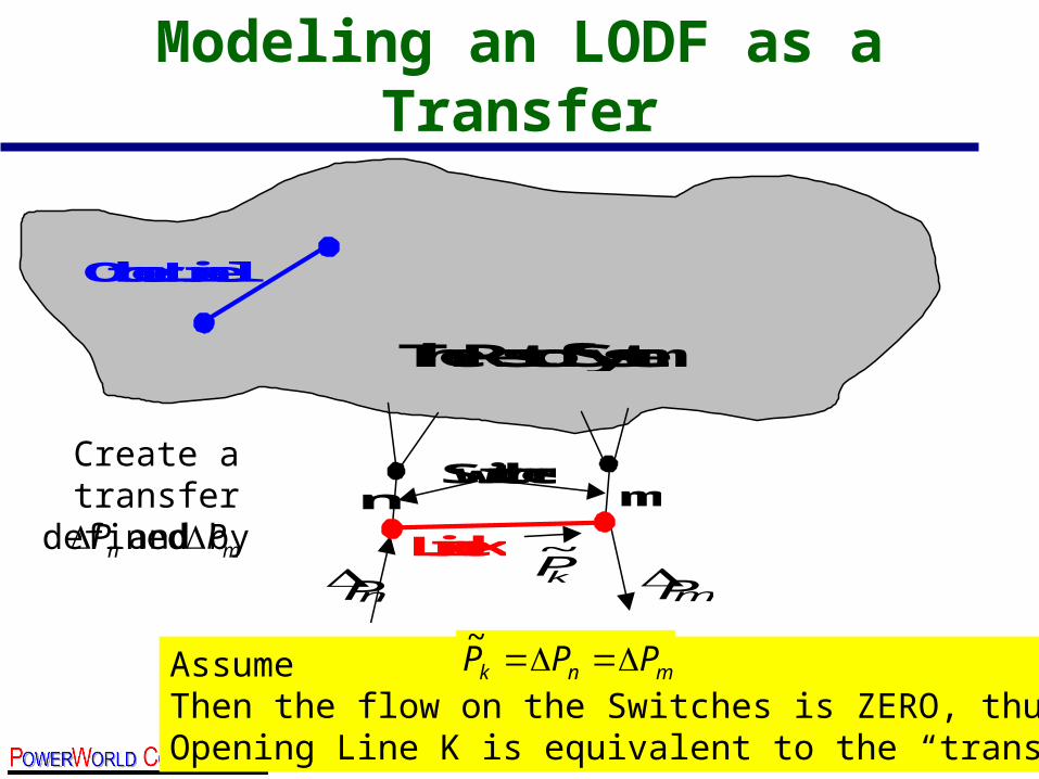
AssumeThen the flow on the Switches is ZERO, thusOpening Line K is equivalent to the “transfer”

Modeling an LODF as a Transfer

Line k

n m

Other Line l

The Rest of System

Pn Pm kP~

Switches

mnk PPP ~

mn PP and

Create a transfer defined by

25

Modeling an LODF as a Transfer

• Thus, setting up a transfer of MW from Bus n to Bus m is linearly equivalent to outaging the transmission line

• Let’s assume we know what is equal to, then we can calculate the values relevant to the LODF–Calculate the relevant values by using PTDFs

for a “transfer” from Bus n to Bus m.

kP~

kP~

26

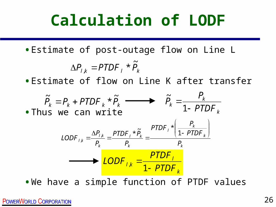
Calculation of LODF

• Estimate of post-outage flow on Line L

• Estimate of flow on Line K after transfer

• Thus we can write

• We have a simple function of PTDF values

klkl PPTDFP~

*,

kkkk PPTDFPP~

*~

k

kk PTDF

PP

1

~

k

k

kl

k

kl

k

klkl P

PTDFP

PTDF

P

PPTDF

P

PLODF

1

*~*,

,

k

lkl PTDF

PTDFLODF

1,

27

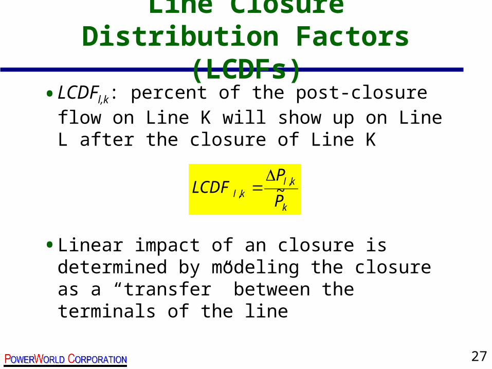
Line Closure Distribution Factors (LCDFs)

• LCDFl,k: percent of the post-closure flow on Line K will show up on Line L after the closure of Line K

• Linear impact of an closure is determined by modeling the closure as a “transfer” between the terminals of the line

k

klkl

P

PLCDF ~

,,

28

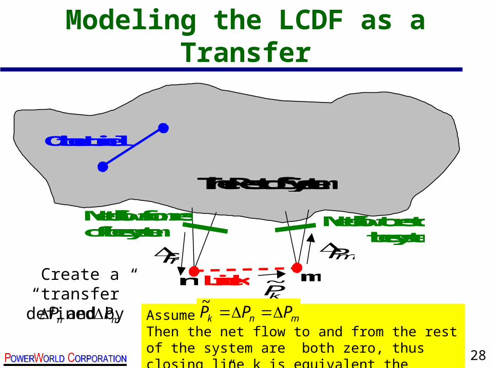
Modeling the LCDF as a Transfer

Line k n m

Other Line l

The Rest of System

Pn Pm

kP~

Net flow from rest of the system

Net flow to rest of the system

AssumeThen the net flow to and from the rest of the system are both zero, thus closing line k is equivalent the “transfer”

mnk PPP ~mn PP and

Create a “transfer” defined by

29

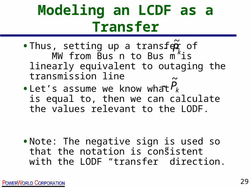
Modeling an LCDF as a Transfer

• Thus, setting up a transfer of MW from Bus n to Bus m is linearly equivalent to outaging the transmission line

• Let’s assume we know what is equal to, then we can calculate the values relevant to the LODF.

• Note: The negative sign is used so that the notation is consistent with the LODF “transfer” direction.

kP~

kP~

30

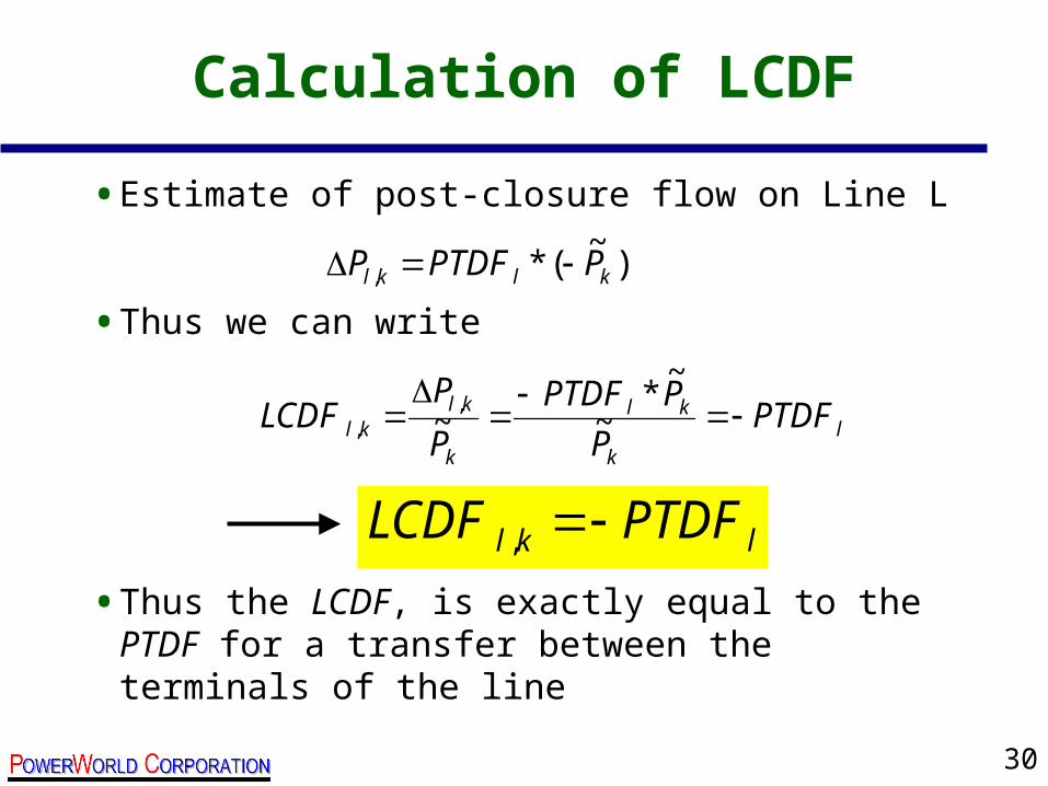
Calculation of LCDF

• Estimate of post-closure flow on Line L

• Thus we can write

• Thus the LCDF, is exactly equal to the PTDF for a transfer between the terminals of the line

)~

(*, klkl PPTDFP

lkl PTDFLCDF ,

l

k

kl

k

klkl PTDF

P

PPTDF

P

PLCDF

~

~*

~,

,

31

Modeling Linear Impact of a Contingency

• Outage Transfer Distribution Factors (OTDFs)–The percent of a transfer that will flow on a branch M

after the contingency occurs

• Outage Flows (OMWs)–The estimated flow on a branch M after the

contingency occurs

1 2 nc . . . . . . M

Contingent Lines 1 through nc Monitored Line M

32

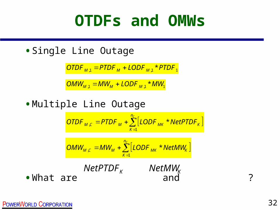
OTDFs and OMWs

• Single Line Outage

• Multiple Line Outage

• What are and ?

11,1, * PTDFLODFPTDFOTDF MMM

11,1, *MWLODFMWOMW MMM

Cn

KKMKMCM NetPTDFLODFPTDFOTDF

1, *

Cn

KKMKMCM NetMWLODFMWOMW

1, *

KNetPTDF KNetMW

33

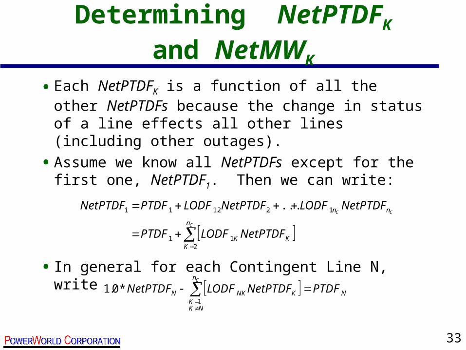
Determining NetPTDFKand NetMWK

• Each NetPTDFK is a function of all the other NetPTDFs because the change in status of a line effects all other lines (including other outages).

• Assume we know all NetPTDFs except for the first one, NetPTDF1. Then we can write:

• In general for each Contingent Line N, write

C

CC

n

KKK

nn

NetPTDFLODFPTDF

NetPTDFLODFNetPTDFLODFPTDFNetPTDF

211

121211 ...

N

n

NKK

KNKN PTDFNetPTDFLODFNetPTDFC

1

*0.1

34

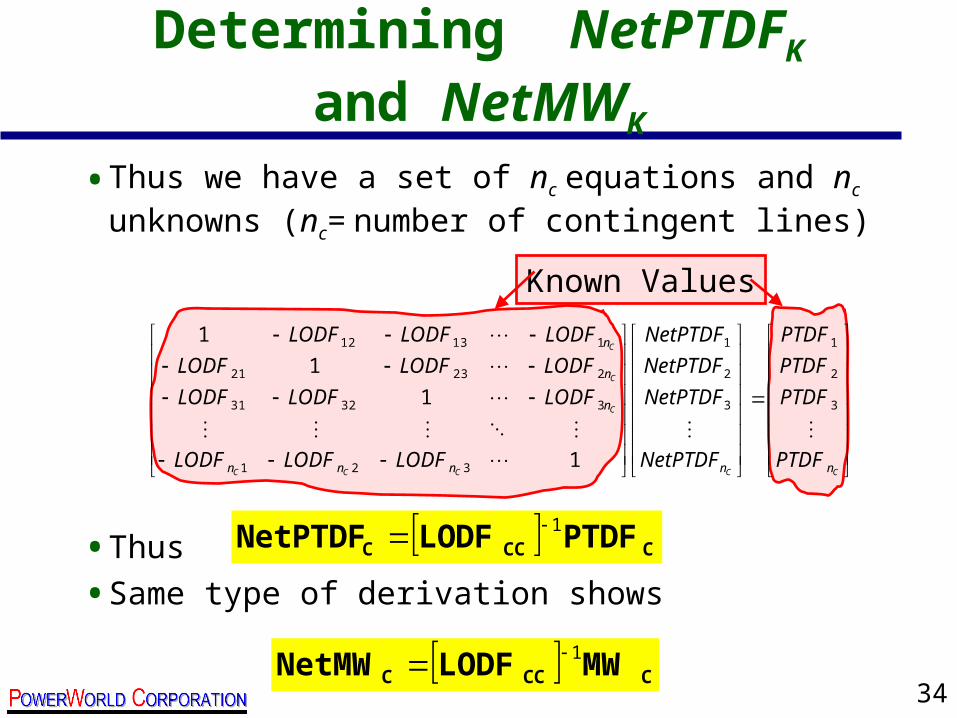
• Thus we have a set of nc equations and nc unknowns (nc= number of contingent lines)

• Thus

• Same type of derivation shows

Determining NetPTDFKand NetMWK

CCCCC

C

C

C

nnnnn

n

n

n

PTDF

PTDF

PTDF

PTDF

NetPTDF

NetPTDF

NetPTDF

NetPTDF

LODFLODFLODF

LODFLODFLODF

LODFLODFLODF

LODFLODFLODF

3

2

1

3

2

1

321

33231

22321

11312

1

1

1

1

CCCC PTDFLODFNetPTDF 1

CCCC MWLODFNetMW 1

Known Values

35

Fast ATC Analysis Goal =Avoid Power Flow Solutions

• When completely solving ATC, the number of power flow solutions required is equal to the product of– The number of contingencies

– The number of iterations required to determine the ATC (this is normally smaller than the number of contingencies)

• We will look at three methods (2 are linearized)– Single Linear Step (fully linearized)

• Perform a single power flow, then all linear (extremely fast)

– Iterated Linear Step (mostly linear, Contingencies Linear)• Requires iterations of power flow to ramp out to the maximum transfer level, but no

power flows for contingencies.

– (IL) then Full AC• Requires iterations of power flow and full solution of contingencies

36

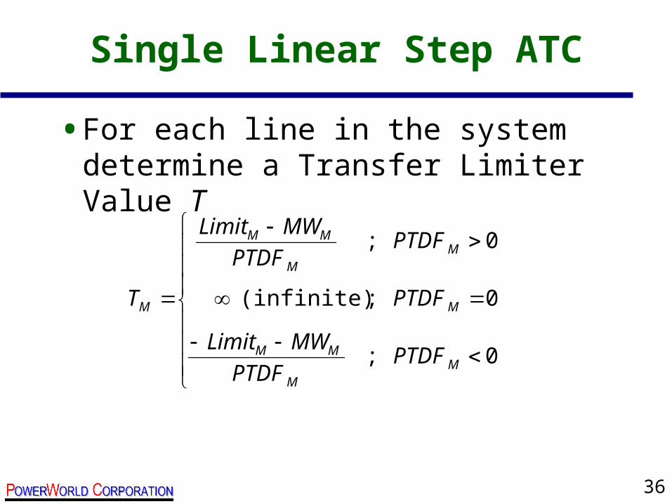
Single Linear Step ATC

• For each line in the system determine a Transfer Limiter Value T

0;

0;(infinite)

0;

MM

MM

M

MM

MM

M

PTDFPTDF

MWLimit

PTDF

PTDFPTDF

MWLimit

T

37

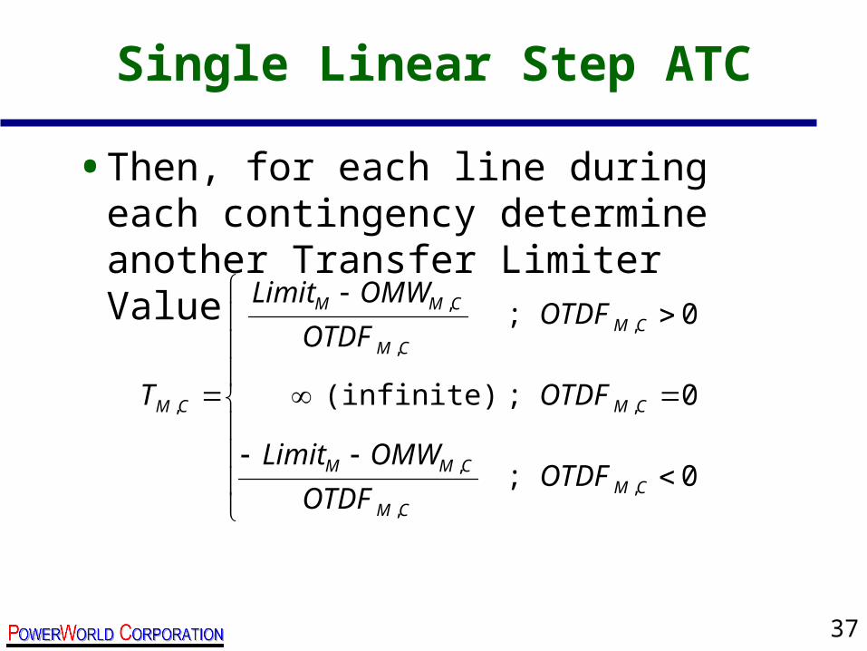
Single Linear Step ATC

• Then, for each line during each contingency determine another Transfer Limiter Value

0;

0;(infinite)

0;

,,

,

,

,,

,

,

CMCM

CMM

CM

CMCM

CMM

CM

OTDFOTDF

OMWLimit

OTDF

OTDFOTDF

OMWLimit

T

38

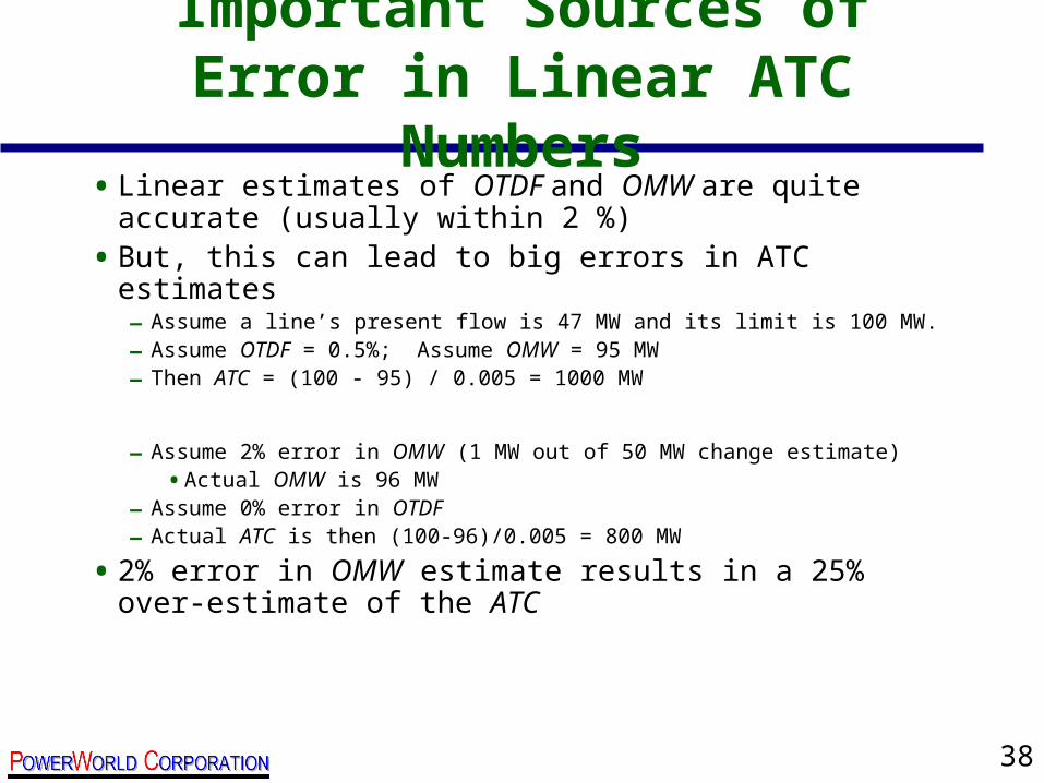
Important Sources of Error in Linear ATC Numbers

• Linear estimates of OTDF and OMW are quite accurate (usually within 2 %)

• But, this can lead to big errors in ATC estimates– Assume a line’s present flow is 47 MW and its limit is 100 MW.

– Assume OTDF = 0.5%; Assume OMW = 95 MW

– Then ATC = (100 - 95) / 0.005 = 1000 MW

– Assume 2% error in OMW (1 MW out of 50 MW change estimate)

• Actual OMW is 96 MW

– Assume 0% error in OTDF

– Actual ATC is then (100-96)/0.005 = 800 MW

• 2% error in OMW estimate results in a 25% over-estimate of the ATC

39

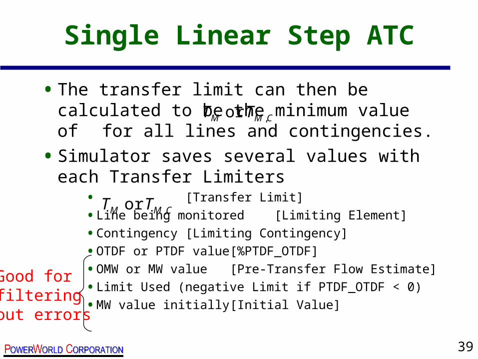
Single Linear Step ATC

• The transfer limit can then be calculated to be the minimum value of for all lines and contingencies.

• Simulator saves several values with each Transfer Limiters

• [Transfer Limit]

• Line being monitored [Limiting Element]

• Contingency [Limiting Contingency]

• OTDF or PTDF value [%PTDF_OTDF]

• OMW or MW value [Pre-Transfer Flow Estimate]

• Limit Used (negative Limit if PTDF_OTDF < 0)

• MW value initially [Initial Value]

CMM TT ,or

CMM TT ,or

Good forfilteringout errors

40

Pros and Cons of the Linear Step ATC

• Single Linear Step ATC is extremely fast– Linearization is quite accurate in modeling the impact

of contingencies and transfers

• However, it only uses derivatives around the present operating point. Thus,– Control changes as you ramp out to the transfer limit

are NOT modeled• Exception: We made special arrangements for Phase Shifters

– The possibility of generators participating in the transfer hitting limits is NOT modeled

• The, Iterated Linear Step ATC takes into account these control changes.

41

Iterated Linear (IL) Step ATC

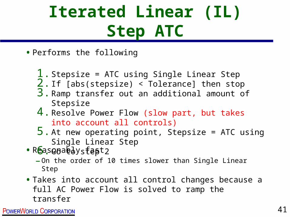
• Performs the following

• Reasonably fast– On the order of 10 times slower than Single Linear Step

• Takes into account all control changes because a full AC Power Flow is solved to ramp the transfer

1. Stepsize = ATC using Single Linear Step 2. If [abs(stepsize) < Tolerance] then stop3. Ramp transfer out an additional amount of Stepsize 4. Resolve Power Flow (slow part, but takes into account all

controls)5. At new operating point, Stepsize = ATC using Single Linear Step6. Go to step 2

42

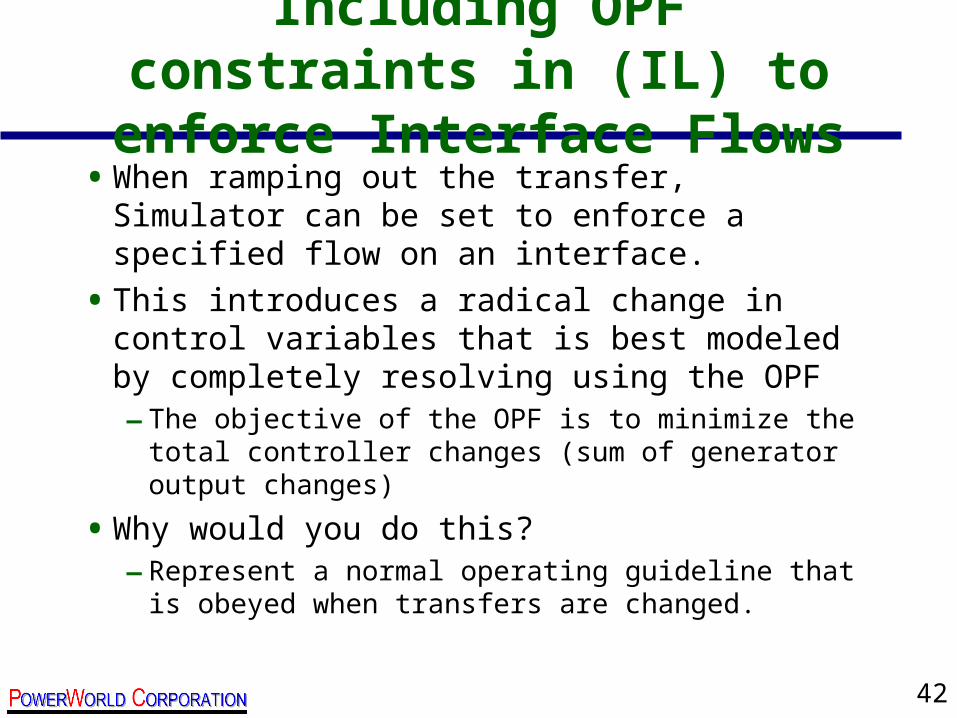
Including OPF constraints in (IL) to enforce Interface Flows

• When ramping out the transfer, Simulator can be set to enforce a specified flow on an interface.

• This introduces a radical change in control variables that is best modeled by completely resolving using the OPF– The objective of the OPF is to minimize the total

controller changes (sum of generator output changes)

• Why would you do this?– Represent a normal operating guideline that is obeyed

when transfers are changed.

43

1000 MW

653 MW

199 MVR

653 MW105 MVR105 MVR

177 MVR 19 MVR

670 MW

30 MW

101 MVR1155 MW

769 MW 26 MVR

26 MVR769 MW

2 MVR 26 MVR 5 MW769 MW

95 MW-45 MVR

1000 MW

653 MW

199 MVR

653 MW105 MVR105 MVR

1000 MW

653 MW

199 MVR

653 MW105 MVR105 MVR

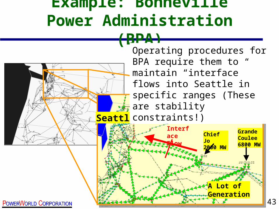
Example: Bonneville Power Administration (BPA)

A Lot ofGeneration

SeattleGrandeCoulee6800 MW

InterfaceFlow Chief Jo

2000 MW

Operating procedures for BPA require them to maintain “interface” flows into Seattle in specific ranges (These are stability constraints!)

44

(IL) then Full AC Method

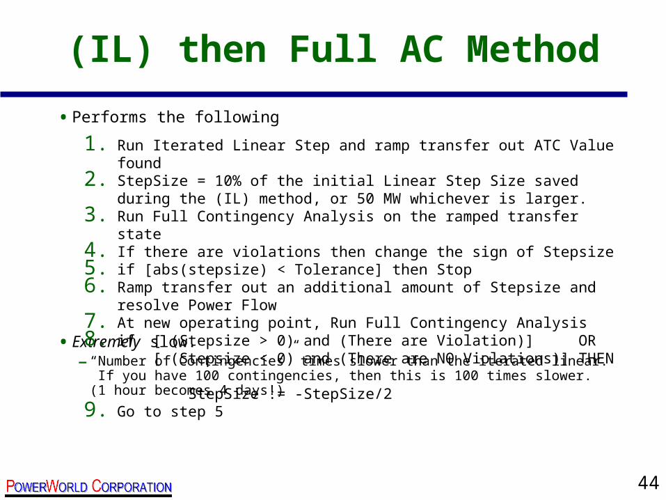
• Performs the following

• Extremely slow.– “Number of Contingencies” times slower than the iterated linear. If you have

100 contingencies, then this is 100 times slower. (1 hour becomes 4 days!)

1. Run Iterated Linear Step and ramp transfer out ATC Value found2. StepSize = 10% of the initial Linear Step Size saved during the (IL) method, or 50

MW whichever is larger.3. Run Full Contingency Analysis on the ramped transfer state4. If there are violations then change the sign of Stepsize5. if [abs(stepsize) < Tolerance] then Stop6. Ramp transfer out an additional amount of Stepsize and resolve Power Flow7. At new operating point, Run Full Contingency Analysis8. if [ (Stepsize > 0) and (There are Violation)] OR

[ (Stepsize < 0) and (There are NO Violations)] THEN StepSize := -StepSize/2

9. Go to step 5

45

Recommendations from PowerWorld’s Experience

• Single Linear Step – Use for all preliminary analysis, and most analysis in

general.

• Iterated Linear Step– Only use if you know that important controls change as you

ramp out to the limit

• (IL) then Full AC– Never use this method. It’s just too slow.

– The marginal gain in accuracy compared to (IL) (less than 2%) doesn’t justify the time requirements

– Remember that ATC numbers probably aren’t any more than 2% accurate anyway! (what limits did you choose, what generation participates in the transfer, etc…)