Embed Size (px)
Citation preview

1
1
Power Systems Engineering Research Center (PSERC )
An NSF Industry / University Cooperative Research Center
PSERC
2
PSERCMission
Universities working with industry and government to find innovative solutions to challenges facing a restructured electric power industry.• Multi-disciplinary (engineering, economics, operations research, etc.)
• Multi-university• Collaborative• Research and education activities

2
3
PSERCPSERC Universities
• Cornell University (lead university)• Arizona State University• University of California at Berkeley• Carnegie Mellon University• Colorado School of Mines• Georgia Institute of Technology• The University Of Illinois at Urbana• Iowa State University• Texas A&M University• Washington State University• University of Wisconsin-Madison
4
PSERCResearch Program
• Three research stems• Markets• Transmission and distribution technologies• Systems
• Leveraged research (such as Consortium for Electric Reliability Technology Solutions)
• Public documents: www.pserc.wisc.edu
3
5
Electric Service Reliability
Fernando L. AlvaradoProfessor, University of WisconsinInvited PresentationInvited PresentationInvited PresentationInvited Presentation43434343rdrdrdrd NARUC ProgramNARUC ProgramNARUC ProgramNARUC ProgramEast Lansing, Michigan, August 15, 2001East Lansing, Michigan, August 15, 2001East Lansing, Michigan, August 15, 2001East Lansing, Michigan, August 15, 2001
6
PSERCOutline
• Traditional reliability concepts• LOLP• n-1 security• Reserve margins
• Reliability in a market context• The Value Of Lost Load (VOLL)
• Some market power issues
4
Traditional reliability concepts
• Loss of load probability (LOLP)• Expected Demand Not Served (EDNS)
• n-1 security• Reserve margins
8
PSERCElectric service reliability
• End-user perspective:• Any involuntary loss of power is a reliability event
• Bulk system perspective:• Any system condition leading to loss of load is a reliability event
• Only those leading to widespread or extended outages are considered true reliability events
• The outage of a component is not an event
5
9
PSERCReliability Time Frames
• The planning time frame• The operations time frame
• Reliability in this timeframe is sometimes called security
• In this talk we will emphasize the operations time frame
10
PSERCLoss of load probability
• A “planning” concept• Based on random outage of generators, what is the probability that the available generators will be insufficient to meet the anticipated load
• Measured in frequency of expected outages
• EDNS extends the concept to consider energy “not served”

6
11
PSERCThe n-1 security criterion
• “The outage of any single piece of equipment shall not result in an uncontrolled loss of load”• A pretty universal and fundamental way of operating the system
• Cost in not in the equation• Sometimes n-2 and n-3 criteria are used
12
PSERCApplying the n-1 criterion
• Outage of any generator does not cause overloads or other problems• n-1 criterion used to establish reserve requirements
• Outage of any line or transformer should not cause any other overloads• If a potential problem exists, system is redispatched for “security reasons” (either via CED, via TLR, or via prices)
7
13
PSERCWhy do systems fail?
• Cascading overloads • A simple line or transformer outage is not enough except in radial situations
• Most distribution systems are radial• Loss of system stability
• Transient or dynamic• Voltage collapse• Insufficiency of generation
14
PSERCReserves
• The loss of any generator shall not cause an uncontrolled loss of load
• The “area control error” (ACE) must be brought under control• NERC has well-defined rules for this• At present the rules are “voluntary”
8
15
PSERCWhat is the ACE?
• To facilitate control, the power system is divided into control areas• All exports and imports are monitored• Every area balances its energy to attain the desired exports or imports
• It also contributes to frequency control• The ACE is the deviation between the intended frequency+exports and the actual values
16
PSERCMore on reserves
• Reserves may have to be locational• They must consider time of response
• Reserves are often classified this way• “Sustainability” attribute of reserves has been underconsidered to date
• The cost of procuring reserves can be quite important
• Reactive reserves are important
9
17
PSERCReserve margins
• “How far are we from a failure under normal conditions”• And how about under contingency conditions
• A contingency is the loss of a component• You must also ask “in what direction”
• How far is the nearest gas station is different from how far is the next gas station
• Often the direction is “total system load”
18
PSERCChoosing reserve margins
• Depends on “largest credible event”• Sometimes the probability of a triggered event is factored in• Play it more conservative during bad weather
• Margins often expressed in terms of size of largest generator or loss of biggest import
10
19
PSERCTemporal classification
• Spinning reserves• Fast-responding, usually instantaneously
• Supplemental reserves• You can bring resources on-line quickly
• Backup reserves• They can be brought on line after some time
Reliability in a market context
• Reliability event occurs when demand exceeds supply• The supply and demand curves do not intersect!
11
21
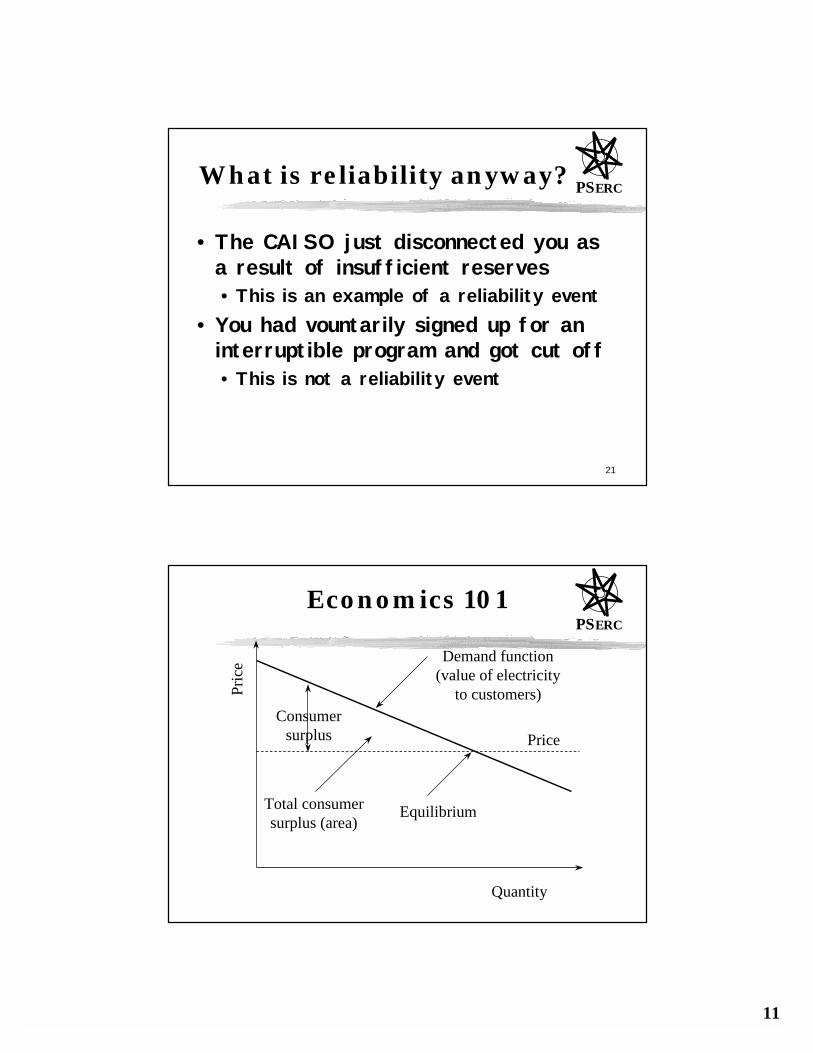
PSERCWhat is reliability anyway?
• The CAISO just disconnected you as a result of insufficient reserves• This is an example of a reliability event
• You had vountarily signed up for an interruptible program and got cut off• This is not a reliability event
PSERCEconomics 101
Quantity
Pric
e
Equilibrium
PriceConsumer
surplus
Demand function(value of electricity
to customers)
Total consumersurplus (area)
12
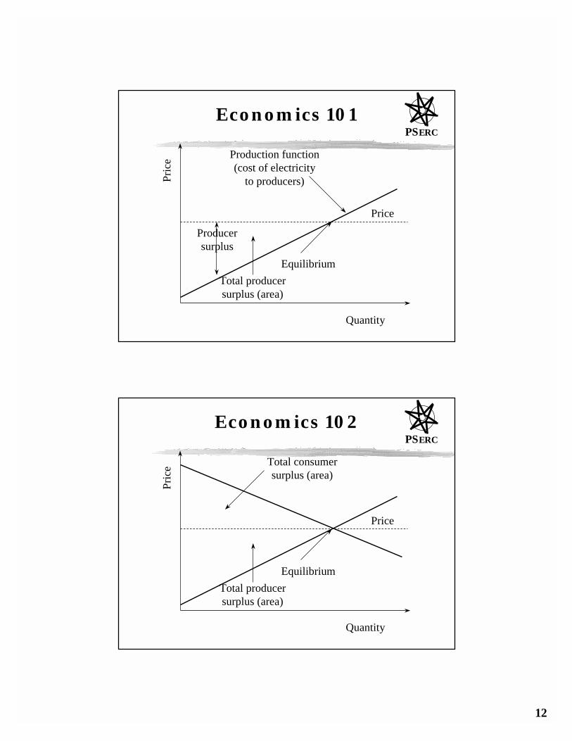
PSERCEconomics 101
Quantity
Pric
e
Equilibrium
Price
Producersurplus
Production function(cost of electricity
to producers)
Total producersurplus (area)
PSERCEconomics 102
Quantity
Pric
e
Equilibrium
Price
Total producersurplus (area)
Total consumersurplus (area)
13
25
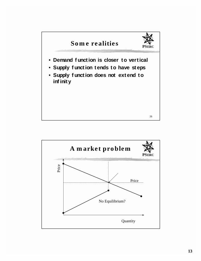
PSERCSome realities
• Demand function is closer to vertical• Supply function tends to have steps• Supply function does not extend to infinity
PSERCA market problem
Quantity
Pric
e
No Equilibrium?
Price
14
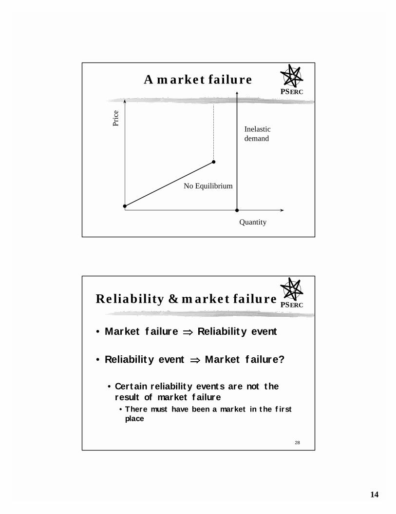
PSERCA market failure
Quantity
Pric
e
No Equilibrium
Inelasticdemand
28
PSERCReliability & market failure
• Market failure ⇒⇒⇒⇒ Reliability event
• Reliability event ⇒⇒⇒⇒ Market failure?
• Certain reliability events are not the result of market failure
• There must have been a market in the first place
15
29
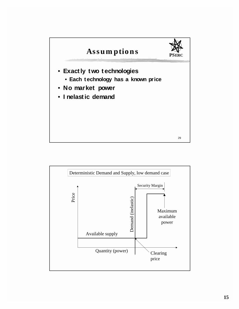
PSERCAssumptions
• Exactly two technologies• Each technology has a known price
• No market power• Inelastic demand
Quantity (power)
Pric
e
Dem
and
(inel
astic
)
Available supply
Clearingprice
Maximumavailable
power
Deterministic Demand and Supply, low demand case
Security Margin
16
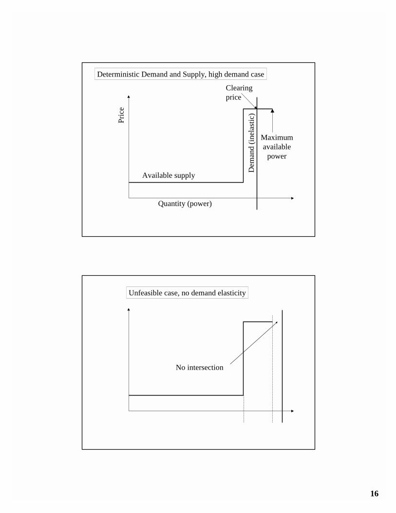
Quantity (power)
Pric
e
Dem
and
(inel
astic
)
Available supply
Clearingprice
Maximumavailable
power
Deterministic Demand and Supply, high demand case
Unfeasible case, no demand elasticity
No intersection
17
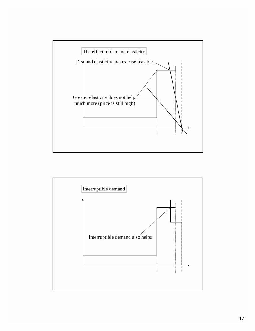
The effect of demand elasticity
Demand elasticity makes case feasible
Greater elasticity does not helpmuch more (price is still high)
Interruptible demand
Interruptible demand also helps
18
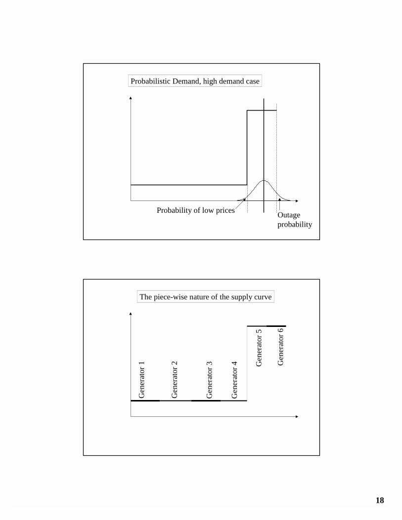
Probabilistic Demand, high demand case
Outageprobability
Probability of low prices
The piece-wise nature of the supply curve
Gen
erat
or 1
Gen
erat
or 2
Gen
erat
or 3
Gen
erat
or 4 G
ener
ator
5
Gen
erat
or 6
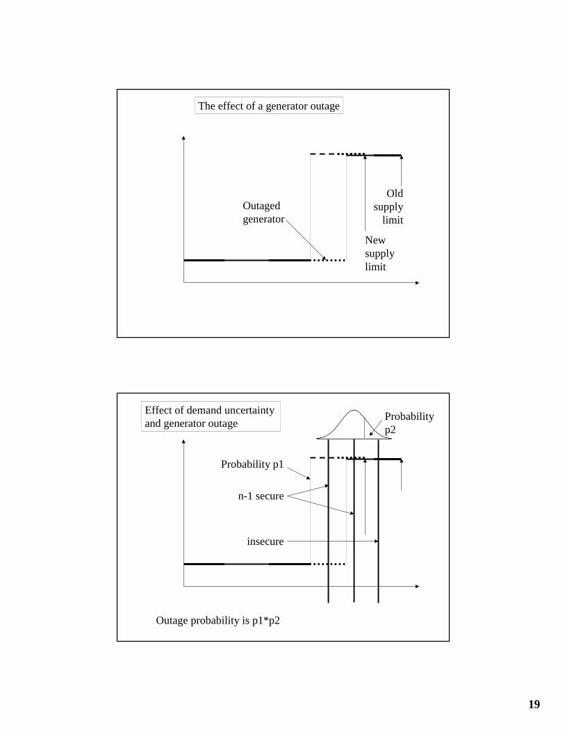
19
The effect of a generator outage
Outagedgenerator
Oldsupply
limit
Newsupplylimit
Effect of demand uncertainty and generator outage
n-1 secure
insecure
Probabilityp2
Outage probability is p1*p2
Probability p1
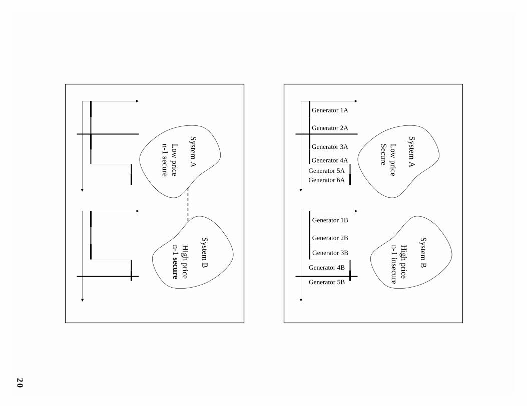
20
System B
System A
Generator 1A
Generator 2A
Generator 3A
Generator 4AGenerator 5AGenerator 6A
Generator 1B
Generator 2B
Generator 3B
Generator 4B
Generator 5B
High price
n-1 insecureLow
priceSecure
System B
System A
High price
n-1 secureLow
pricen-1 secure
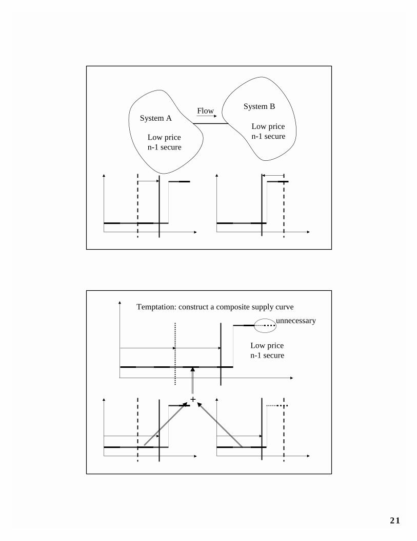
21
System BSystem A
Low pricen-1 secureLow price
n-1 secure
Flow
Temptation: construct a composite supply curve
+
Low pricen-1 secure
unnecessary
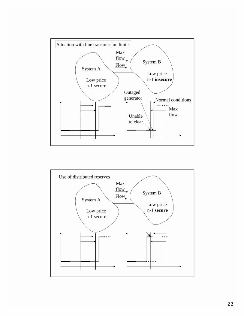
22
Flow
Normal conditions
System BSystem A
Low pricen-1 insecureLow price
n-1 secure
Situation with line transmission limitsMaxflow
Maxflow
Outagedgenerator
Unableto clear
System BSystem A
Flow
Maxflow
Use of distributed reserves
Low pricen-1 secureLow price
n-1 secure
23
45
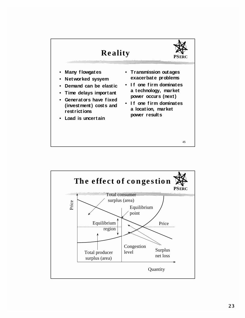
PSERCReality
• Many flowgates• Networked sysyem• Demand can be elastic• Time delays important• Generators have fixed
(investment) costs and restrictions
• Load is uncertain
• Transmission outages exacerbate problems
• If one firm dominates a technology, market power occurs (next)
• If one firm dominates a location, market power results
PSERCThe effect of congestion
Quantity
Pric
e
Price
Total producersurplus (area)
Total consumersurplus (area)
Congestionlevel Surplus
net loss
Equilibriumregion
Equilibriumpoint
24
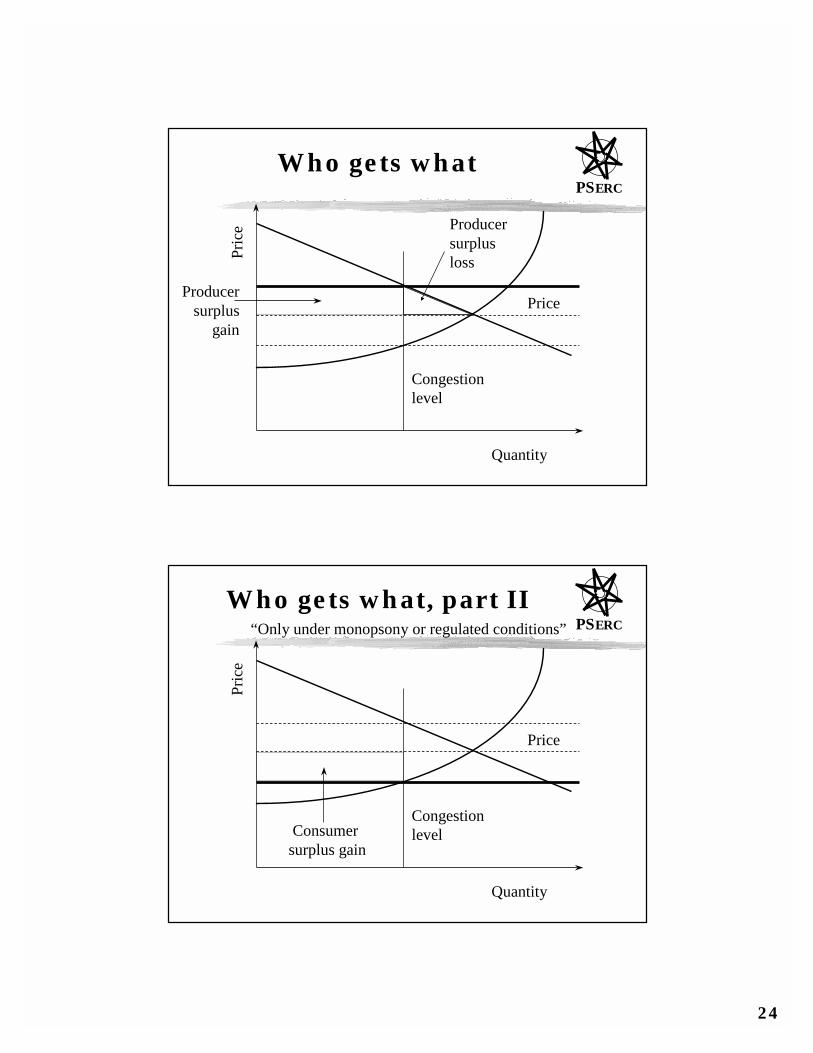
PSERCWho gets what
Quantity
Pric
e
Price
Congestionlevel
Producersurplus
gain
Producersurplusloss
PSERCWho gets what, part II
Quantity
Pric
e
Price
Consumer surplus gain
Congestionlevel
“Only under monopsony or regulated conditions”
25
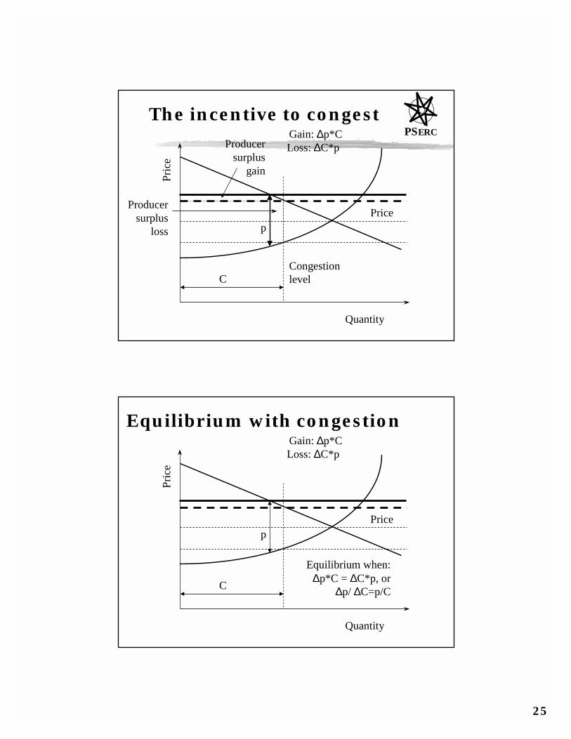
PSERCThe incentive to congest
Quantity
Pric
e
Price
Congestionlevel
Producersurplus
loss
Producersurplus
gain
Gain: ∆p*CLoss: ∆C*p
p
C
Equilibrium with congestion
Quantity
Pric
e
Price
Gain: ∆p*CLoss: ∆C*p
Equilibrium when: ∆p*C = ∆C*p, or
∆p/ ∆C=p/C
p
C
26
PSERCThe effect of congestion
• Congestion creates “gaming” opportunities• Producers have an incentive to congest
• (Up to a point)• The only unambiguous way to characterize the effect of congestion is to look at net surplus loss• Translated: when we compute congestion costs, we do not care who incurs them
52
PSERCAdditional remarks
• Two-technology suppliers can lead to higher than marginal prices as the knee of the supply curve is approached
• Larger number of suppliers reduces this effect
• Market power studies should consider investment recovery issues
• Transmission congestion makes matters worse!!
27
53
PSERCFeatures of the example
• Only two areas (one flowgate)• Radial• Demand is inelastic• Time delays are not an issue• Generators have no startup/shutdown costs or restrictions or minimum power levels
54
PSERCObservations
• Demand elasticity is important• Locational aspects of reserves matter
• LMP for reserves• Ramping rates matter• In deregulated markets only units explicitly
committed to reserves are available• In regulated markets and in PJM all units are
• Reliability requires that we increase supply• Standby charges tend to reduce supply (Tim
Mount)
28
55
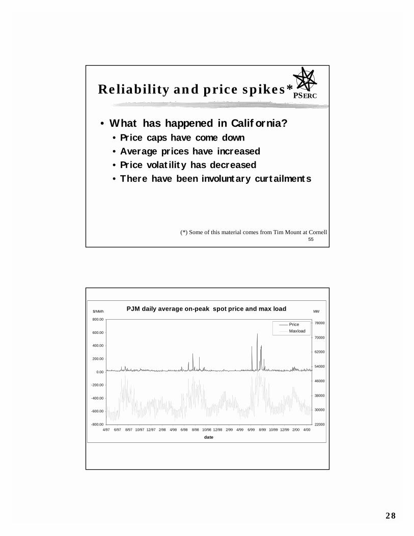
PSERCReliability and price spikes*
• What has happened in California?• Price caps have come down• Average prices have increased• Price volatility has decreased• There have been involuntary curtailments
(*) Some of this material comes from Tim Mount at Cornell
PJM daily average on-peak spot price and max load
-800.00
-600.00
-400.00
-200.00
0.00
200.00
400.00
600.00
800.00
4/97 6/97 8/97 10/97 12/97 2/98 4/98 6/98 8/98 10/98 12/98 2/99 4/99 6/99 8/99 10/99 12/99 2/00 4/00
date
22000
30000
38000
46000
54000
62000
70000
78000PriceMaxload
$/MWh MW
29
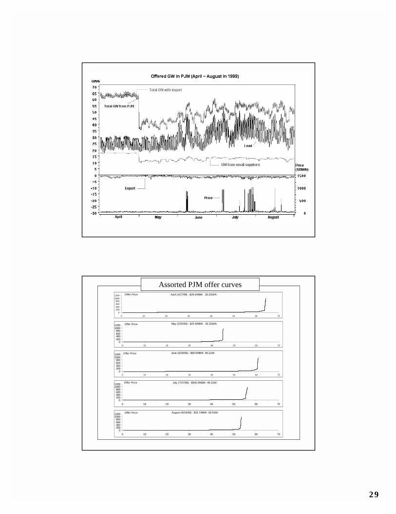
PJM Offer Curves at 5pm from April to August (last Tuesday)
April (4/27/99) : $29.4/MWh 28.2GW/h
0200400600800
10001200
0 10 20 30 40 50 60 70
Offer Price
May (5/25/99) : $25.9/MWh 30.3GW/h
0200400600800
10001200
0 10 20 30 40 50 60 70
Offer Price
June (6/29/99) : $59.5/MWh 48.1GW
0200400600800
10001200
0 10 20 30 40 50 60 70
Offer Price
July (7/27/99) : $935.0/MWh 49.2GW
0200400600800
10001200
0 10 20 30 40 50 60 70
Offer Price
August (8/24/99) : $33.7/MWh 38.5GW
0200400600800
10001200
0 10 20 30 40 50 60 70
Offer Price
Assorted PJM offer curves

30
59
PSERCObservations
• Price spikes have developed not so much under high load conditions as under tight reserve conditions
• For suppliers that own more than one technology, there are strong incentives to withhold capacity
• There is a strong connection between reserves and reliability (and market power)
Market Power?
• The ability to raise prices significantly above the efficient economic equilibrium
• Disclaimer: the slides that follow are not really a market power study but rather they represent a simplified illustration of how higher prices could result as a result of market concentration.
31
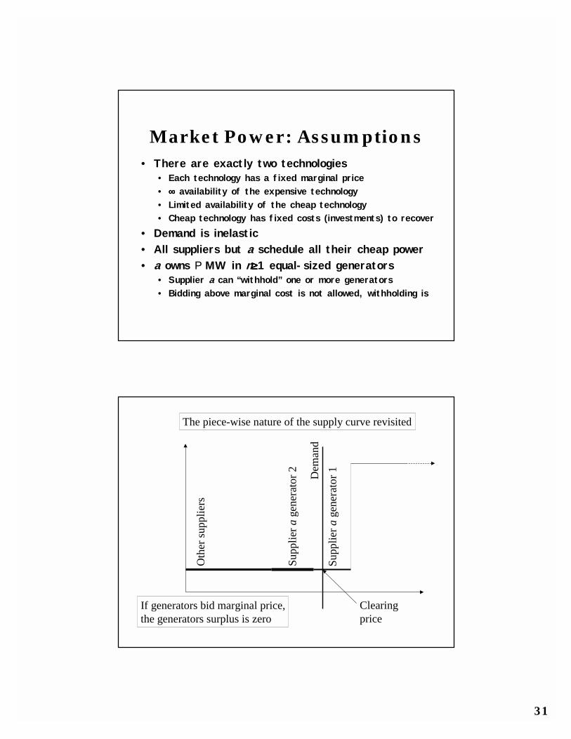
Market Power: Assumptions• There are exactly two technologies
• Each technology has a fixed marginal price• ∞∞∞∞ availability of the expensive technology• Limited availability of the cheap technology• Cheap technology has fixed costs (investments) to recover
• Demand is inelastic• All suppliers but a schedule all their cheap power• a owns P MW in n≥≥≥≥1 equal-sized generators
• Supplier a can “withhold” one or more generators• Bidding above marginal cost is not allowed, withholding is
The piece-wise nature of the supply curve revisited
Oth
er su
pplie
rs
Supp
lier a
gene
rato
r 1Dem
and
Clearingprice
If generators bid marginal price,the generators surplus is zero
Supp
lier a
gene
rato
r 2
32
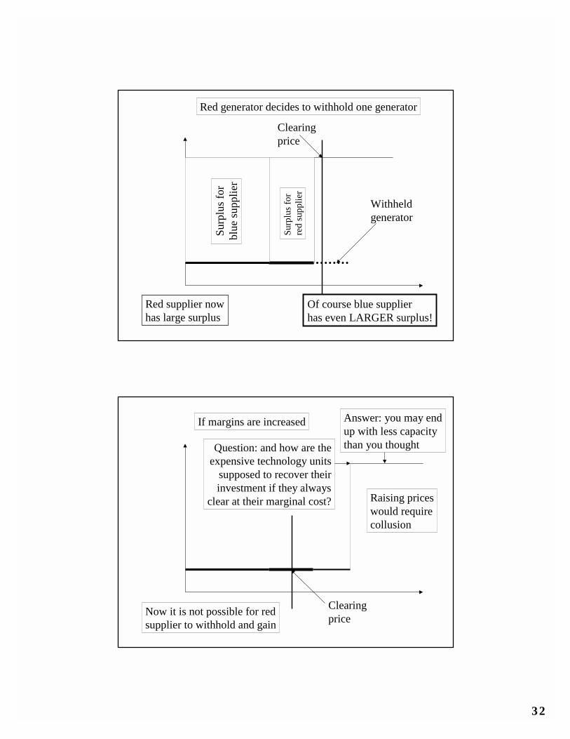
Red generator decides to withhold one generator
Withheldgenerator
Clearingprice
Surp
lus f
orre
d su
pplie
rRed supplier nowhas large surplus
Of course blue supplierhas even LARGER surplus!
Surp
lus f
orbl
ue su
pplie
r
If margins are increased
ClearingpriceNow it is not possible for red
supplier to withhold and gain
Raising priceswould requirecollusion
Question: and how are theexpensive technology units
supposed to recover theirinvestment if they always
clear at their marginal cost?
Answer: you may endup with less capacitythan you thought
33
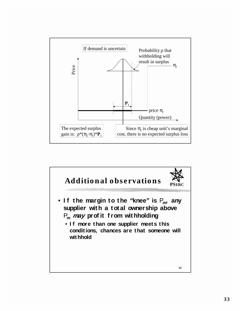
If demand is uncertain
The expected surplusgain is: p*(π2-π1)*P1
Probability p thatwithholding willresult in surplus
π2
P1
price π1
Quantity (power)
Pric
e
Since π1 is cheap unit’s marginalcost, there is no expected surplus loss
66
PSERCAdditional observations
• If the margin to the “knee” is Pm, any supplier with a total ownership above Pm may profit from withholding• If more than one supplier meets this conditions, chances are that someone will withhold
34
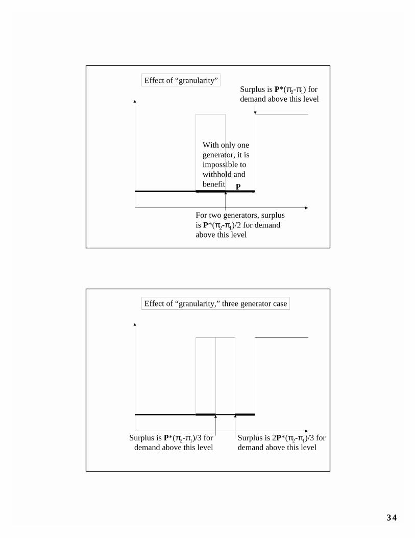
For two generators, surplusis P*(π2-π1)/2 for demandabove this level
Effect of “granularity”
With only onegenerator, it isimpossible towithhold andbenefit P
Surplus is P*(π2-π1) fordemand above this level
Effect of “granularity,” three generator case
Surplus is P*(π2-π1)/3 fordemand above this level
Surplus is 2P*(π2-π1)/3 fordemand above this level
35
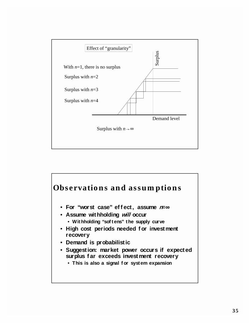
Effect of “granularity”
Surp
lus
With n=1, there is no surplus
Surplus with n=2
Surplus with n=3
Surplus with n=4
Surplus with n→∞
Demand level
Observations and assumptions
• For “worst case” effect, assume n=∞∞∞∞• Assume withholding will occur
• Withholding “softens” the supply curve• High cost periods needed for investment
recovery• Demand is probabilistic• Suggestion: market power occurs if expected
surplus far exceeds investment recovery• This is also a signal for system expansion
36
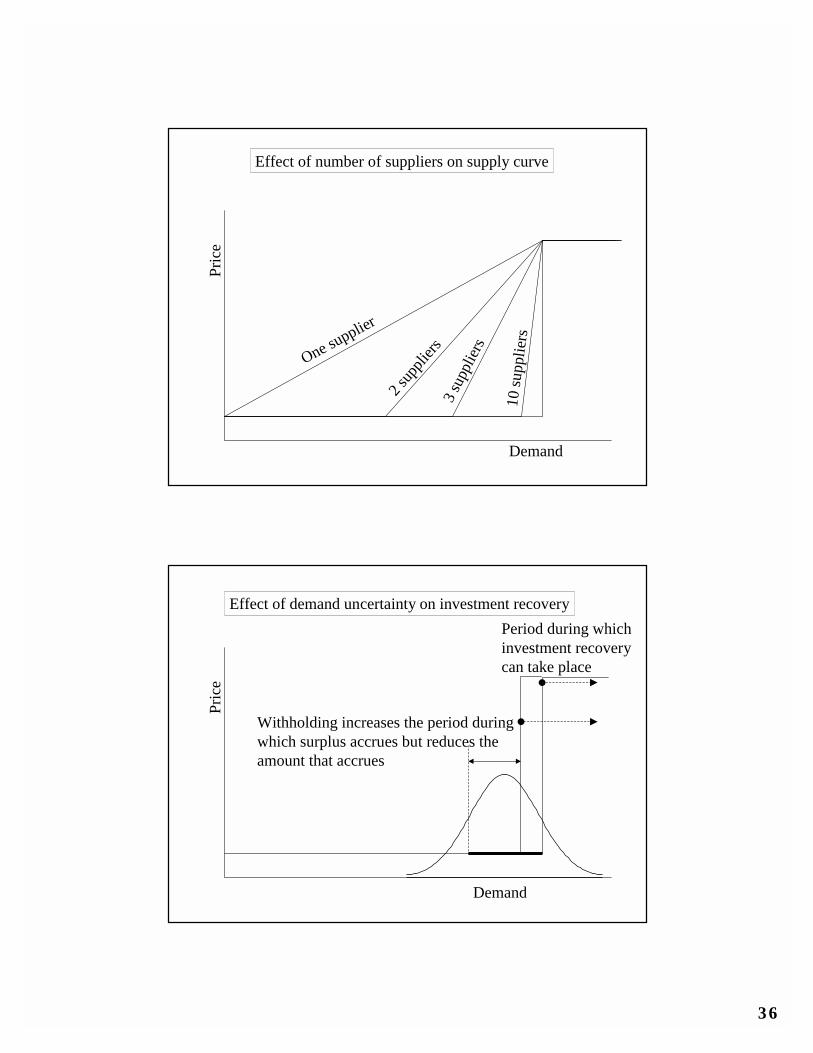
Effect of number of suppliers on supply curve
One supplier
2 sup
pliers
3 su
pplie
rs
10 su
pplie
rs
Demand
Pric
ePr
ice
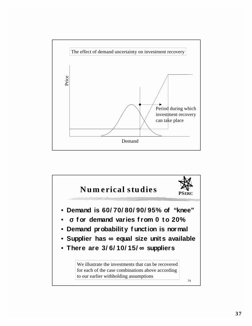
Demand
Period during whichinvestment recoverycan take place
Effect of demand uncertainty on investment recovery
Withholding increases the period duringwhich surplus accrues but reduces theamount that accrues
37
Pric
e
Demand
Period during whichinvestment recoverycan take place
The effect of demand uncertainty on investment recovery
74
PSERCNumerical studies
• Demand is 60/70/80/90/95% of “knee”• σσσσ for demand varies from 0 to 20%• Demand probability function is normal• Supplier has ∞∞∞∞ equal size units available• There are 3/6/10/15/∞∞∞∞ suppliers
We illustrate the investments that can be recoveredfor each of the case combinations above accordingto our earlier withholding assumptions
38
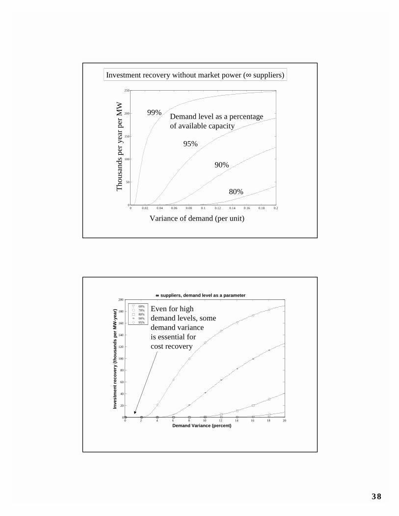
0 0.02 0.04 0.06 0.08 0.1 0.12 0.14 0.16 0.18 0.20
50
100
150
200
250
80%
Variance of demand (per unit)
Investment recovery without market power (∞ suppliers)
Thou
sand
s per
yea
r per
MW
90%
95%
99% Demand level as a percentageof available capacity
0 2 4 6 8 10 12 14 16 18 200
20
40
60
80
100
120
140
160
180
200
Demand Variance (percent)
Inve
stm
ent r
ecov
ery
(thou
sand
s pe
r MW
-yea
r)
∞∞∞∞ suppliers, demand level as a parameter
60%70%80%90%95%
Even for highdemand levels, somedemand varianceis essential forcost recovery
39
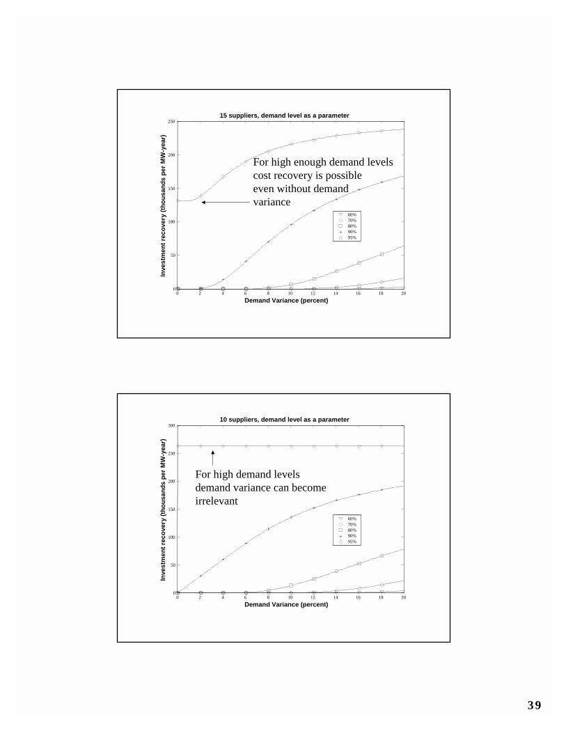
0 2 4 6 8 10 12 14 16 18 200
50
100
150
200
250
Demand Variance (percent)
Inve
stm
ent r
ecov
ery
(thou
sand
s pe
r MW
-yea
r)
15 suppliers, demand level as a parameter
60%70%80%90%95%
For high enough demand levelscost recovery is possibleeven without demand variance
0 2 4 6 8 10 12 14 16 18 200
50
100
150
200
250
300
Demand Variance (percent)
Inve
stm
ent r
ecov
ery
(thou
sand
s pe
r MW
-yea
r)
10 suppliers, demand level as a parameter
60%70%80%90%95%
For high demand levelsdemand variance can becomeirrelevant
40
0 2 4 6 8 10 12 14 16 18 200
50
100
150
200
250
300
350
400
Demand Variance (percent)
Inve
stm
ent r
ecov
ery
(thou
sand
s pe
r MW
-yea
r)
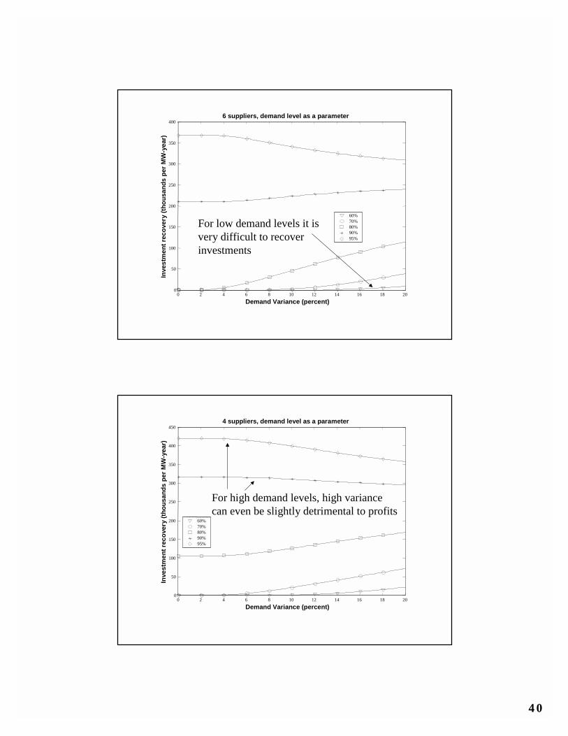
6 suppliers, demand level as a parameter
60%70%80%90%95%
For low demand levels it isvery difficult to recoverinvestments
0 2 4 6 8 10 12 14 16 18 200
50
100
150
200
250
300
350
400
450
Demand Variance (percent)
Inve
stm
ent r
ecov
ery
(thou
sand
s pe
r MW
-yea
r)
4 suppliers, demand level as a parameter
60%70%80%90%95%
For high demand levels, high variancecan even be slightly detrimental to profits
41
0 2 4 6 8 10 12 14 16 18 200
50
100
150
200
250
300
350
400
450
Demand Variance (percent)
Inve
stm
ent r
ecov
ery
(thou
sand
s pe
r MW
-yea
r)
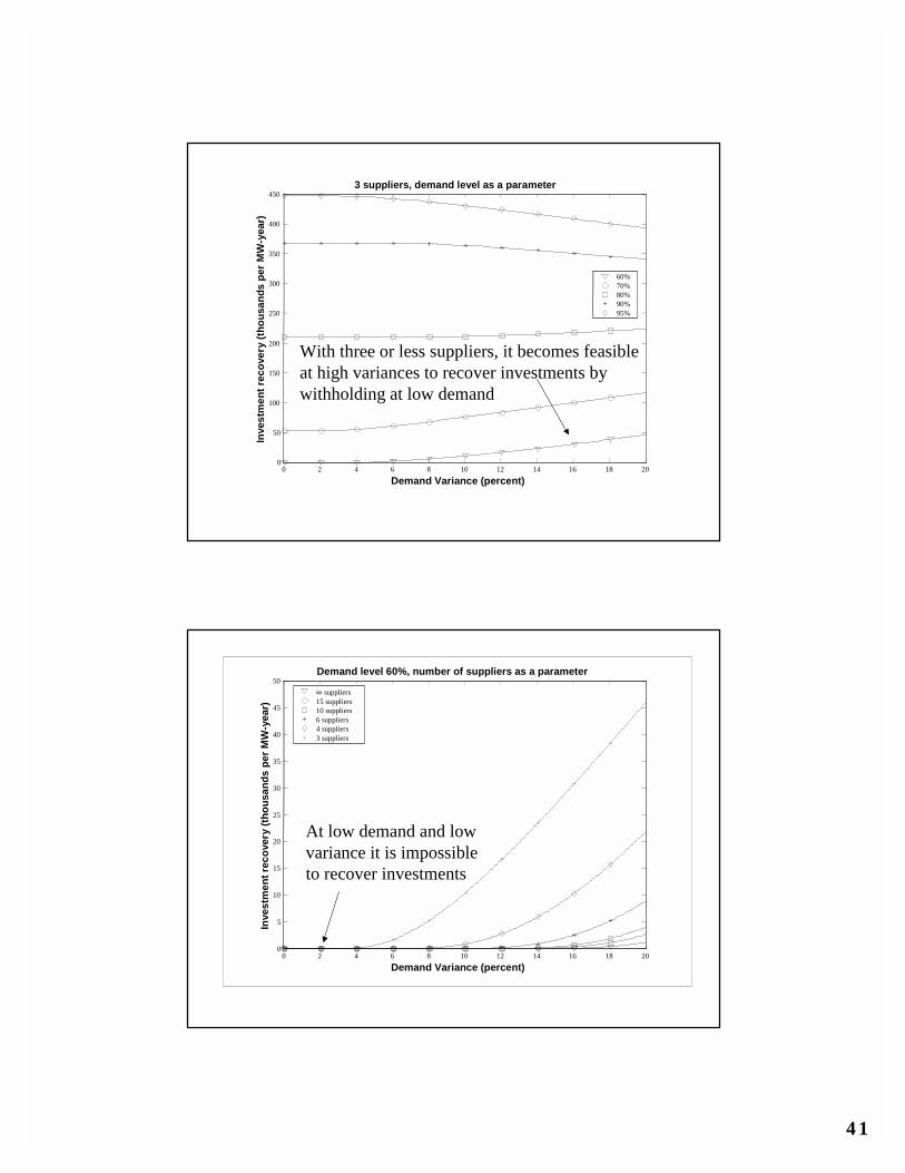
3 suppliers, demand level as a parameter
60%70%80%90%95%
With three or less suppliers, it becomes feasibleat high variances to recover investments bywithholding at low demand
0 2 4 6 8 10 12 14 16 18 200
5
10
15
20
25
30
35
40
45
50
Demand Variance (percent)
Inve
stm
ent r
ecov
ery
(thou
sand
s pe
r MW
-yea
r)
Demand level 60%, number of suppliers as a parameter
∞ suppliers15 suppliers 10 suppliers 6 suppliers 4 suppliers 3 suppliers
At low demand and lowvariance it is impossibleto recover investments
42
0 2 4 6 8 10 12 14 16 18 200
20
40
60
80
100
120
Demand Variance (percent)
Fixe
d co
st re
cove
ry (t
hous
ands
per
MW
-yea
r)
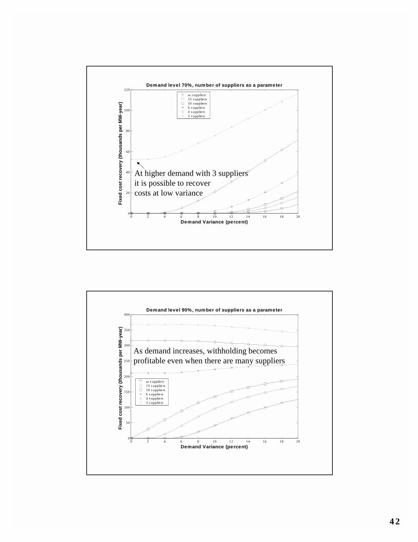
Demand level 70%, number of suppliers as a parameter
∞ s upplie rs15 s upplie rs 10 s upplie rs 6 s upplie rs 4 s upplie rs 3 s upplie rs
At higher demand with 3 suppliersit is possible to recovercosts at low variance
0 2 4 6 8 10 12 14 16 18 200
50
100
150
200
250
300
350
400
Demand Variance (percent)
Fixe
d co
st re
cove
ry (t
hous
ands
per
MW
-yea
r)
Demand level 90%, number of suppliers as a parameter
∞ s upplie rs15 s upplie rs 10 s upplie rs 6 s upplie rs 4 s upplie rs 3 s upplie rs
As demand increases, withholding becomesprofitable even when there are many suppliers
43
0 2 4 6 8 10 12 14 16 18 200
50
100
150
200
250
300
350
400
450
Demand Variance (percent)
Fixe
d co
st re
cove
ry (t
hous
ands
per
MW
-yea
r)
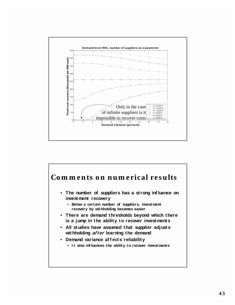
Demand level 95%, number of suppliers as a parameter
∞ s upplie rs15 s upplie rs 10 s upplie rs 6 s upplie rs 4 s upplie rs 3 s upplie rs
Only in the caseof infinite suppliers is it
impossible to recover costs
Comments on numerical results
• The number of suppliers has a strong influence on investment recovery• Below a certain number of suppliers, investment
recovery by withholding becomes easier• There are demand thresholds beyond which there
is a jump in the ability to recover investments• All studies have assumed that supplier adjusts
withholding after learning the demand• Demand variance affects reliability
• It also influences the ability to recover investments
44
87
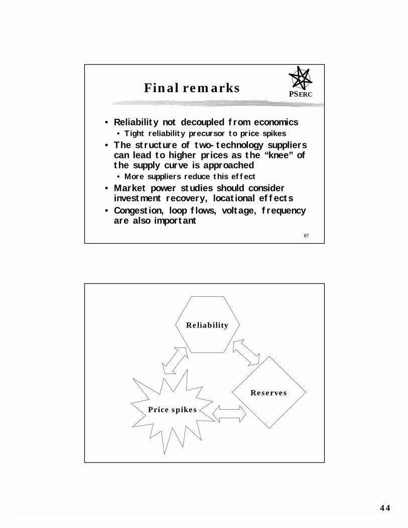
PSERCFinal remarks
• Reliability not decoupled from economics• Tight reliability precursor to price spikes
• The structure of two-technology suppliers can lead to higher prices as the “knee” of the supply curve is approached• More suppliers reduce this effect
• Market power studies should consider investment recovery, locational effects
• Congestion, loop flows, voltage, frequency are also important
Reliability
Reserves
Price spikes