entropy

Article

Refined Multiscale Entropy Using FuzzyMetrics: Validation and Application toNociception Assessment †

José F. Valencia 1,* , Jose D. Bolaños 1, Montserrat Vallverdú 2,3,4 , Erik W. Jensen 5,Alberto Porta 6,7 and Pedro L. Gambús 8,9

1 Department of Electronic Engineering, Universidad de San Buenaventura, Cali 760033, Colombia2 Department of Automatic Control, Universitat Politècnica de Catalunya, 08028 Barcelona, Spain3 Center for Biomedical Engineering Research, Universitat Politècnica de Catalunya, 08028 Barcelona, Spain4 CIBER of Bioengineering, Biomaterials and Nanomedicine (CIBER-BBN), 08028 Barcelona, Spain5 Research and Development Department, Quantium Medical SL, 08302 Mataró, Spain6 Department of Biomedical Sciences for Health, University of Milan, 20133 Milan, Italy7 Department of Cardiothoracic-Vascular Anesthesia and Intensive Care, IRCCS Policlinico San Donato,

San Donato Milanese, 20097 Milan, Italy8 Systems Pharmacology Effect Control & Modeling (SPEC-M) Research Group, Department of Anesthesia,

Hospital CLINIC de Barcelona, 08036 Barcelona, Spain9 Department of Anesthesia and Perioperative Care, University of California San Francisco (UCSF),

San Francisco, CA 94143, USA* Correspondence: jfvalenc@usbcali.edu.co; Tel.: +57-301-5749049† This paper is an extended version of an abstract presented in the 40th Annual International Conference of

the IEEE Engineering in Medicine and Biology Society (EMBC’18), Honolulu, HI, USA, 17–21 July 2018.

Received: 2 July 2019; Accepted: 16 July 2019; Published: 18 July 2019�����������������

Abstract: The refined multiscale entropy (RMSE) approach is commonly applied to assess complexityas a function of the time scale. RMSE is normally based on the computation of sample entropy(SampEn) estimating complexity as conditional entropy. However, SampEn is dependent on thelength and standard deviation of the data. Recently, fuzzy entropy (FuzEn) has been proposed,including several refinements, as an alternative to counteract these limitations. In this work, FuzEn,translated FuzEn (TFuzEn), translated-reflected FuzEn (TRFuzEn), inherent FuzEn (IFuzEn), andinherent translated FuzEn (ITFuzEn) were exploited as entropy-based measures in the computationof RMSE and their performance was compared to that of SampEn. FuzEn metrics were applied tosynthetic time series of different lengths to evaluate the consistency of the different approaches. Inaddition, electroencephalograms of patients under sedation-analgesia procedure were analyzed basedon the patient’s response after the application of painful stimulation, such as nail bed compression orendoscopy tube insertion. Significant differences in FuzEn metrics were observed over simulationsand real data as a function of the data length and the pain responses. Findings indicated that FuzEn,when exploited in RMSE applications, showed similar behavior to SampEn in long series, but itsconsistency was better than that of SampEn in short series both over simulations and real data.Conversely, its variants should be utilized with more caution, especially whether processes exhibit animportant deterministic component and/or in nociception prediction at long scales.

Keywords: fuzzy entropy; conditional entropy; complexity; electroencephalography; pain assessment;refined multiscale entropy; sample entropy; sedation-analgesia

Entropy 2019, 21, 706; doi:10.3390/e21070706 www.mdpi.com/journal/entropy

Entropy 2019, 21, 706 2 of 21

1. Introduction

Recently, fuzzy entropy (FuzEn) has been proposed as an entropy measure that is more consistentand less dependent on the data length [1,2]. Indeed, FuzEn applys the concept of “fuzzy sets” andmembership functions, introduced by Zadeh in 1965, to characterize input–output relations withstochastic components [3]. Some applications of FuzEn in biomedical signal processing has beenpresented in [4–8]. In order to improve the performance of FuzEn in short time series, several variationshave been included in its computation. Some of them are centered and averaged fuzzy entropy [9] andinherent fuzzy entropy [10].

FuzEn, as sample entropy (SampEn) and other entropy rates, gives only a single scale representationof the behavior of a time series. However, these measurements can be extended to provide a multiscaleassessment of irregularity of the time series. Refined multiscale entropy (RMSE), proposed in [11], is atechnique that uses SampEn as an entropy-based measure in order to quantify the complexity of a timeseries in different time scales, which has been applied in processing of electrocardiogram (ECG) andelectroencephalogram (EEG) signals [12–15]. Computation of RMSE is similar to multiscale entropy(MSE) [16] except for two significant modifications: (i) RMSE improves the procedure applied toremove the fast time scales in the signal, avoiding the aliasing, and; (ii) it modifies the coarse-grainingprocedure to avoid an artificial decrease of the entropy as the fast time scales in the signal are eliminated,which is caused by the reduction of the standard deviation that is generated by the filtering process.

Characterization of time series by means of RMSE requires relatively long length series, whichincreases the computation time and makes difficult the implementation of this algorithm in real timemonitoring systems. The implementation of FuzEn and its variants, which offer an entropy-basedmeasure that is less dependent on the data length, emerges as alternative to the traditional SampEnfor the real-time multiscale analysis. This can be very useful, for example, to monitor patients, usingphysiological signals as the EEG in critical settings such as critical care units. For example, undersedation/anesthesia during surgery the assessment of complexity of the EEG via RMSE was founduseful for monitoring the level of consciousness and preventing pain [15]. The assessment of EEGcomplexity as a function of time scales using of RMSE is motivated by the observation that the EEGcontains oscillations at particular frequency bands, and these oscillations become slower and moreregular at higher doses of intravenous anesthetic such as the propofol. In this sense, slower and lessunpredictable oscillations can be associated with a deeper state of sedation [15].

The aim of this study is to compare the performance of SampEn and FuzEn metrics, with itsdifferent variants, when they are exploited for a multiscale analysis by means of RMSE. Synthetic andexperimental time series are analyzed in order to evaluate the behavior of RMSE metrics in signalswith different characteristics: stochastic without or with long-range correlation, stochastic but partiallypredictable, fully predictable determinist or chaotic. The study also involves the analysis of time serieswith different lengths and the application of RMSE to assess the prediction probability of pain responsein patients under sedation-analgesia.

2. Methods

2.1. Database

2.1.1. Synthetic Time Series

Synthetic signals were categorized in:

(a) Type-1, which included (i) Gaussian white noise (GWN) to simulate a fully unpredictableprocess; (ii) 1/f noise or pink noise (1/f) to generate a stochastic signal with long-range correlation;(iii) second-order autoregressive process (AR025), driven by GWN, to simulate a partiallypredictable stochastic process. The AR025 was shaped to have a power spectrum peak withcentral frequency at 0.25 cycles per sample and pole modulus p = 0.98. The parameters in AR025were proposed to check the ability of RMSE to avoid aliasing when the downsampling procedure

Entropy 2019, 21, 706 3 of 21

is applied [11]. Sixty realizations of 100,000 samples were generated for each process (GWN, 1/f,and AR025).

(b) Type-2, which included signals generated from (i) logistic map (LM), defined by xn+1 = axn(1− xn),where the parameter ”a” controls the value of the samples such that the signals converges to asingle fixed point if a ≤ 3, oscillates if 3 < a < 3.54, and becomes increasingly chaotic and more andmore complex structures emerge for larger a [17]. In this study, LM with values of the parametera equals to 3.5 (oscillation condition, LM-3.5), 3.7 (chaotic condition, LM-3.7), and 3.9 (chaoticcondition, LM-3.9) were considered; (ii) Henon map (HM), defined by xn+1 = 1−αxn

2 + βxn−1 [18],was exploited to conduct more detailed exploration of the chaotic dynamics, using α = 1.4 andβ = 0.3. Thirty realizations of 50,000 samples were generated for each process (LM-3.5, LM-3.7,LM-3.9, and HM).

2.1.2. Experimental Time Series

The different approaches of RMSE were applied to EEG signals recorded from 378 patients undersedation-analgesia during an ultrasonographic endoscopy (USE) of the upper gastrointestinal tract.USE is a procedure with an approximate duration of 1 h, which includes periods of stability in theconcentration of the anesthetic drugs, allowing the outcome of painful stimulus to be studied in relationwith the level of sedation. This exploration required at least two endoscopy tube insertions: the firstcomponent carrying a regular gastroscope and a second component carrying the needle for biopsy.This study was approved by the Ethic Committee of Clinical Research of Hospital Clinic de Barcelonaand all patients signed a written informed consent.

Patients were routinely monitored in the USE room. A single channel of the raw EEG signal wasacquired using three electrodes: the positive electrode in the middle forehead; the negative electrodein the malar bone, and; the reference electrode in the left forehead. The recorded EEGs had an averageduration of 60 m and were sampled at 900 samples per second with a resolution of 16 bits per sample.Propofol and remifentanil were infused as, respectively, anesthetic and analgesic agents by meansof a target-controlled infusion system (FreseniusVial, Chemin de Fer, Béziers, France). The Ramsaysedation scale (RSS) score [19] was evaluated, by the attending anesthesiologist, at random timesduring the procedure. Random times were decided instead of a predefined schedule to avoid thatfactors associated with time, such as the infusion volume of propofol and remifentanil, could affect theresults of the RSS measurements. Table 1 contains information about the annotated RSS scores in thedatabase, which are between 2 and 6.

Table 1. Observed categorical responses in the database.

Groups Score Description No. EEG Windows

2 ≤ RSS ≤ 5

RSS = 2 The patient is awake, quiet and cooperative 422RSS = 3 The patient is drowsy but responds to commands 641RSS = 4 The patient is asleep with brisk response to stimulus 428RSS = 5 The patient is asleep with sluggish response to stimulus 360

RSS = 6 No response (absence of movement) to firm nail-bed pressure. 782

GAG = 0 Absence of nausea reflex after endoscopy tube insertion 411

GAG = 1 Presence of nausea reflex after endoscopy tube insertion 125

No. EEG windows: number of EEG segments with a duration between 50 and 60 s recorded just before the responseannotation according to RSS or GAG classification.

After the application of painful stimulation, two observed categorical responses were selectedin the database (see Table 1): (i) the presence (RSS score between 2 and 5) or the absence (RSS = 6)of movement after nail bed compression, and; (ii) the presence or absence of gag reflex (GAG) afterendoscopy tube insertion, where GAG = 1 corresponds to a positive nausea reflex, while GAG = 0corresponds to no response after tube insertion. As the evaluation of RSS scores was done at randomtimes, and the duration of every exploration was determined by the procedure per se, the number of

Entropy 2019, 21, 706 4 of 21

RSS measurements were not equal in all patients (the median number of RSS score evaluations was 11per patient). The number of GAG evaluations was between one and two per patient, according to thenumber of endoscopy tube insertion.

The next preprocessing steps were applied to EEG signals:

(i) They were resampled at 128 Hz after applying a band-pass finite impulse response (FIR) filter of10th order with cut-off frequencies of 0.1–45 Hz, in order to limit the EEG signal to the traditionalfrequency bands: δ (0.1–4 Hz), θ (4–8 Hz), α (8–14 Hz), and β (14–30 Hz).

(ii) The filtered and resampled EEG signals were divided into windows of 1-min duration taken justbefore the response annotation according to RSS or GAG classification.

(iii) The 1-min EEG segments were associated to the correspondent annotated response (RSS orGAG) by considering that the sedation level should remain constant if the plasma concentrationof remifentanil (CeRemi) and propofol (CeProp) remains unvaried. In this work, CeRemiand CeProp were considered constant if the variation of them (∆CeRemi, ∆CeProp), betweenthe first and the last second of the 1-min length window, was ∆CeRemi < 0.1 ng/mL and∆CeProp < 0.1 µg/mL.

(iv) If CeRemi and CeProp were not constant during the 1-min length window, the window wasmaintained but cut at the sample where the conditions were satisfied. If the total useful lengthwas less than 50 s the overall segment was excluded from the analysis.

(v) Windows of EEG were filtered with a filter based on the analytic signal envelope in order toreduce high-amplitude peaks of noise [20].

(vi) If the difference between adjacent samples was higher than 10% of the mean of the differences ofthe previous ten samples, the window was cut at the sample where the artifact was detected. If thetotal useful length was less than 50 s the overall segment was excluded from the analysis. Afterthat, only the EEG windows with a duration between 50 and 60 s were included in the analysis.

Table 1 contains information about the number of EEG windows exploited in the present studyfor each annotated response.

2.2. SampEn and Fuzzy Approaches as Entropy Rates

Let x ={x(i), i = 1, . . . , N

}be a time series where i represents the number of the sample and N is the

length of the series, any estimate of an entropy rate (rate of information generation) is based on a methodfor measuring the probability that two patterns of length m, xm(i) = (x(i), x(i− 1), . . . , x(i−m + 1)) andxm( j) = (x( j), x( j− 1), . . . , x( j−m + 1)), that are similar in the m-dimensional phase-space continuebeing similar after adding a new sample in the pattern, i.e., xm+1(i + 1) and xm+1( j + 1) are also similarin the (m + 1)-dimensional phase-space. In this sense, entropy rates allow the regularity of the timeseries x(i) to be quantified, showing high values for irregular or unpredictable series (series with lowprobability that two similar patterns xm(i) and xm( j) remain similar after adding new samples) andlow values for regular or predictable series.

2.2.1. SampEn

In SampEn [21], two patterns (xm(i), xm( j)) are considered similar or indistinguishable if thedistance (dm

ij ) between them is less than a tolerance parameter r in the multidimensional phase-space. Inthis sense, the pattern similarity is determined by the Heaviside function Θ(dm

ij − r) given in Equation (1),which acts like a two-state classifier that generates two possible categories: the patterns are similaror not.

Θ(dm

ij − r)=

1, i f dmij ≤ r, patterns are similar

0, i f dmij > r, patterns are dissimilar

. (1)

Entropy 2019, 21, 706 5 of 21

The distance dmij is defined as:

dmij = max

{∣∣∣(x(i) − x( j)∣∣∣, ∣∣∣x(i− 1) − x( j− 1)

∣∣∣, . . . , ∣∣∣x(i−m + 1) − x( j−m + 1)∣∣∣}, (2)

namely the maximum absolute difference between the corresponding scalar components of the patternsxm(i) and xm( j) (Chebyshev distance). According to [21], SampEn is defined as Equation (3):

SampEn(m, r, N) = −ln(

Amr

Bmr

), (3)

where:

Bmr =

1N −m

N−m∑i=1

1N −m− 1

N−m∑j=1, j,i

Θ(dmij − r), (4)

Amr =

1N −m

N−m∑i=1

1N −m− 1

N−m∑j=1, j,i

Θ(dm+1i j − r). (5)

Bmr represents the probability that two patterns will match for m samples, and Am

r the probabilitythat two patterns will match for m + 1 samples. The parameter r is usually set as a percentage ofthe standard deviation (SD) of the time series [22], which allows series with different amplitudes tobe compared.

2.2.2. FuzEn

Considering that in the real world the limits between categories may be ambiguous, thus makingthe decision on whether a pattern completely belongs to a specific category difficult, FuzEn employs afuzzy membership function to obtain the degree of similarity between two patterns of length m [1,2].The family of fuzzy functions should include the following characteristics: (i) continuous functions inorder to avoid that the similarity change abruptly; (ii) convex functions to guarantee that self-similarityis the maximum. In FuzEn, the degree of similarity Dm

ij = λ(dmij , n, r) between two patterns xm(i) and

xm( j) is determined by the following fuzzy membership function [1,4]:

λ(dmij , n, r) = exp

−

(dm

ij

)n

r

, (6)

where dmij is the Chebyshev distance between patterns given in Equation (2), r is the tolerance parameter,

and n defines the membership function shape. The membership function corresponds to a Gaussianfunction for n = 2, and to rectangular function for n = ∞. Similar to the definition of SampEn, theprobability that two patterns xm(i) and xm( j) or xm+1(i) and xm+1( j) will match is given, respectively, as

ϕmr =

1N −m

N−m∑i=1

1N −m− 1

N−m∑j=1, j,i

Dmij

, (7)

ϕm+1r =

1N −m

N−m∑i=1

1N −m− 1

N−m∑j=1, j,i

Dm+1i j

. (8)

Finally, FuzEn can be estimated by:

FuzEn(m, r, N) = − ln

ϕm+1r

ϕmr

. (9)

Entropy 2019, 21, 706 6 of 21

In this work, n = 2 was taken as a fixed parameter. It is important to mention that, although inprevious works [1,2,4] xm(i) is generalized by removing a baseline, in the present study FuzEn wascomputed without removing a baseline of xm(i).

2.2.3. Increasing Consistency of FuzEn Estimate

According to [9], although FuzEn offers a more accurate, more consistent, and less dependent onthe data length entropy rate, the length of the series is still an important factor in the precision of FuzEn.In order to address this issue, authors in [9] presented new approaches to calculate FuzEn. These triedto improve FuzEn precision by increasing the number of patterns that are used in the computation,without changing the original length of the series. In this work, two of those approaches were takeninto account: translated FuzEn (TFuzEn) and translated-reflected FuzEn (TRFuzEn).

TFuzEn calculates entropy rate in the same way as FuzEn but defines xm(i) by eliminating themean value of the m-patterns, which can increase the number of similar patterns. The procedure toeliminate the baseline takes the vector xm(i) and subtracts from each component the temporal meancomputed over the entire pattern as follows:

xm(i) = (x(i), x(i + 1), . . . , x(i + m− 1)) − (µ(i),µ(i), . . . ,µ(i)), (10)

where µ(i) is defined as

µ(i) =1m

m−1∑j=0

x(i + j). (11)

The second approach given in [9] involves one additional transformation over the m-dimensionalpatterns, in order to increase the matches of similar patterns. The additional transformation is “reflection”that implies to perform a reflection operation on xm(i), resulting in the reflected subsequence xm

R(i)over the translated pattern as follows:

xmR(i) = (x(i + m− 1), x(i + m− 2), . . . , x(i + 1), x(i)) − (µ(i),µ(i), . . . ,µ(i)), (12)

leading to the elimination of the mean value of the reflected m-dimensional pattern and to thecomputation of TRFuzEn.

2.2.4. Eliminating Trends before FuzEn Computation

Inherent FuzEn (IFuzEn) [10] computes inherent functions, namely intrinsic mode functions(IMFs), obtained from the empirical mode decomposition (EMD), for eliminating superimposed trendsin time series [23–28]. As superimposed trends in physiological signals is very common, and thesetrends could affect the estimation of entropy-based analysis by increasing the standard deviationof the signal, IFuzEn was proposed to increase the reliability of complexity evaluation in realisticEEG applications [10]. Indeed, before applying fuzzy entropy-based methods, IFuzEn implementsa preprocessing stage to eliminate superimposed trends in the time series. In this work, FuzEn andTFuzEn were applied on time series after trend filtering, and they were represented as IFuzEn andITFuzEn, respectively. The concepts about EMD and IMFs are described in Appendix A.

2.3. MSE and RMSE

RMSE is a technique based on the MSE approach [16], which applies SampEn as a function of timescale (TS) in order to perform a multiscale irregularity assessment. In order to do that, MSE followsthe next three steps:

Entropy 2019, 21, 706 7 of 21

(a) Elimination of the fast temporal scales to focus on gradually slower time scales, applying alow-pass finite impulse response (FIR) filter. This FIR filter is based on the average of TS samples,as it is indicated in Equation (13):

xTS( j) =1

TS

TS−1∑k=0

x( j− k), 1 ≤ j ≤ N, (13)

where xTS( j) represents the original series x(i) filtered at the time scale TS. This filter has (i) slowroll-off of the main lobe; (ii) large transition band; (iii) important side lobes, and; (iv) cutoff

frequency fc = 0.5/TS cycles per sample.(b) Downsampling the filtered series xTS( j) by the scale factor TS, so that xTS( j) has the same time

duration of x(i) but with a smaller number of samples as a function of the factor TS. Due tothe large transition band and the important side lobes, the FIR filter given in Equation (13) isinefficient to prevent aliasing when the filtered series are downsampled [11], and therefore, signalswith high-power frequency components, near the center frequency of 0.25 cycles per sample,could generate artifactual components in the downsampled signals.

(c) Calculation of the SampEn in each filtered series xTS( j), according to the Section 2.2.1. In MSE,the tolerance parameter r is fixed as a percentage of the SD of the original series x(i) (usually 15%)and it is kept constant for all the series xTS( j). Due to that, and considering that the SD of filteredseries is reduced by the low-pass filtering procedure, MSE measures not only the variations ofsignals regularity with TS but also the variations in the SD of the series xTS( j).

RMSE introduces two substantial variations in relation with MSE:

(a) The suboptimal FIR filter of MSE is substituted with a sixth order low-pass Butterworth filter toobtain the filtered series xTS( j). This Butterworth filter has the following characteristics: (i) flatresponse in the pass band; (ii) faster roll-off; (iii) no side lobes in the stop band, and; (iv) cutoff

frequency fc = 0.5/TS cycles per sample. This filter, in comparison with the FIR filter given inEquation (13), limits as much as possible the aliasing for any TS during downsampling.

(b) The tolerance parameter r, used for comparing patterns, is updated for each time scale accordingto an assigned fraction of the SD of each filtered series xTS( j). Therefore, RMSE does not dependon the reduction, generated by the low-pass filtering procedure, of the SD of the xTS( j). We makereference to [11] for specific details on the method.

In the present study, RMSE was applied as a technique of multiscale analysis according to(i) the original definition of RMSE (i.e., using a low-pass Butterworth filter, downsampling, andapplying SampEn with tolerance parameter r updated for each time scale over the filtered series), and;(ii) replacing SampEn with FuzEn approaches as FuzEn, TFuzEn, TRFuzEn, IFuzEn, and ITFuzEn.RMSE in its several variants was computed at different TS of the proposed synthetic and experimentaltime series. According to previous works [11–16], in this study r = 0.15 × SD and m = 2 were taken asfixed parameters (in SampEn and FuzEn approaches) to compare RMSE values of the synthetic seriesfor different lengths N. In order to evaluate how the tolerance parameter r affects the performance ofRMSE values of the EEG signals, this parameter was also varied between 0.10 and 0.30 in steps of 0.05.

The different time scales in RMSE can be associated with the traditional EEG-frequency bands δ,θ, α, and β. Indeed, since EEG signals were resampled to 128 Hz, the time scale TS = 1 correspondsto the original EEG signal (with theoretical frequencies from 0 to Nyquist frequency ( fN), i.e.,128/2 = 64 Hz), TS = 2 contains frequencies from 0 to fN/TS = 64/2 = 32 Hz, TS = 3 contains frequenciesfrom 0 to fN/3 = 21.3 Hz, and so on. Therefore, the following approximate association betweenEEG-frequency bands and TS was done: (i) β band corresponds to 2 ≤ TS ≤ 5; (ii) α band correspondsto 5 ≤ TS ≤ 8; (iii) θ band corresponds to 8 ≤ TS ≤ 16, and; (iv) δ band corresponds to TS ≥ 16.

Entropy 2019, 21, 706 8 of 21

Statistical Analysis

In this work, synthetic time series x(i) (see Section 2.1.1) of N = 10,000, N = 1000, and N = 100were analyzed with RMSE. Time scales varied from TS = 1 to TS = 20. Bearing in mind that the lengthof the filtered series xTS( j) is reduced by the scale factor TS, the shorter series (with TS = 20) forN = 10,000 was of 500 samples, for N = 1000 was of 50 samples, and for N = 100 was of five samples.Consistency of RMSE values, in relation to the length N of the series, was evaluated graphically. In thissense, the RMSE metric was consistent whether the plots of RMSE values in different synthetic timeseries held the same relative behavior for different values of N. In other words, if the RMSE values of atime series x1(i) were higher than the RMSE values of a time series x2(i), for a specific TS and length N,that situation had to be maintained for the same TS at different values of N.

The prediction probability score (Pk) was applied to measure how well RMSE of EEG signalpredicted the pain response of the patients. The Pk was proposed in [29] as statistical measurement toassess the performance of anesthetic depth indicators. Indeed, given two random data points withdifferent observed anesthetic states, Pk is the probability that the values of a monitor or indicator inthose data points predict correctly the observed anesthetic states, namely.

Pk =Pc + Ptx/2

Pc + Pd + Ptx, (14)

where Pc, Pd, and Ptx are the respective probabilities of concordance, discordance or x-only tie, betweenthe values of an indicator and the observed anesthetic states. Pk values ranges from 0 to 1, where(i) Pk = 0.5 represents a complete randomness (concordance equal to discordance); (ii) 0.5 < Pk < 1,concordance is more likely than discordance; (iii) Pk = 1 corresponds to perfect concordance (Pd andPtx are both equal to zero); (iv) 0 < Pk < 0.5, concordance is less likely than discordance; (v) Pk = 0means perfect discordance (Pc and Ptx are both equal to zero).

In this work, EEG segments were classified according to the noxious stimuli applied to the patientduring the USE procedure, as follows (see Table 1):

(a) Response after a firm nail-bed pressure: (i) group 2 ≤ RSS ≤ 5, which included patients thatmoved (feel pain) in response to the noxious stimuli; (ii) group with RSS = 6, which did not movein response to the noxious stimuli.

(b) Response after endoscopy tube insertion: (i) group with GAG = 1, which felt pain; (ii) group withGAG = 0, which did not feel pain.

3. Results

3.1. RMSE of Synthetic Time Series

RMSE, using SampEn, FuzEn, TFuzEn, TRFuzEn, IFuzEn, and ITFuzEn, was calculated on allthe realizations of the synthetic time series that were defined in Section 2.1.1. For this analysis,r = 0.15 × SD and m = 2 were taken as fixed parameters in SampEn and FuzEn approaches in order tocompare RMSE values of the synthetic series for different lengths N.

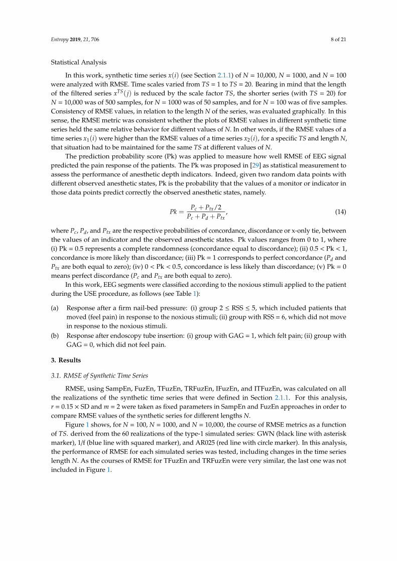
Figure 1 shows, for N = 100, N = 1000, and N = 10,000, the course of RMSE metrics as a functionof TS. derived from the 60 realizations of the type-1 simulated series: GWN (black line with asteriskmarker), 1/f (blue line with squared marker), and AR025 (red line with circle marker). In this analysis,the performance of RMSE for each simulated series was tested, including changes in the time serieslength N. As the courses of RMSE for TFuzEn and TRFuzEn were very similar, the last one was notincluded in Figure 1.

Entropy 2019, 21, 706 9 of 21

Entropy 2019, 21, 706 8 of 20

𝑃𝑘 = 𝑃 + 𝑃 2⁄𝑃 + 𝑃 + 𝑃 , (14)

where 𝑃 , 𝑃 , and 𝑃 are the respective probabilities of concordance, discordance or x-only tie, between the values of an indicator and the observed anesthetic states. Pk values ranges from 0 to 1, where (i) Pk = 0.5 represents a complete randomness (concordance equal to discordance); (ii) 0.5 < Pk < 1, concordance is more likely than discordance; (iii) Pk = 1 corresponds to perfect concordance (𝑃 and 𝑃 are both equal to zero); (iv) 0 < Pk < 0.5, concordance is less likely than discordance; (v) Pk = 0 means perfect discordance (𝑃 and 𝑃 are both equal to zero).

In this work, EEG segments were classified according to the noxious stimuli applied to the patient during the USE procedure, as follows (see Table 1):

(a) Response after a firm nail-bed pressure: (i) group 2 ≤ RSS ≤ 5, which included patients that moved (feel pain) in response to the noxious stimuli; (ii) group with RSS = 6, which did not move in response to the noxious stimuli. (b) Response after endoscopy tube insertion: (i) group with GAG = 1, which felt pain; (ii) group with GAG = 0, which did not feel pain.

3. Results

3.1. RMSE of Synthetic Time Series

RMSE, using SampEn, FuzEn, TFuzEn, TRFuzEn, IFuzEn, and ITFuzEn, was calculated on all the realizations of the synthetic time series that were defined in Section 2.1.1. For this analysis, r = 0.15 × SD and m = 2 were taken as fixed parameters in SampEn and FuzEn approaches in order to compare RMSE values of the synthetic series for different lengths N.

Figure 1 shows, for N = 100, N = 1000, and N = 10,000, the course of RMSE metrics as a function of 𝑇𝑆 derived from the 60 realizations of the type-1 simulated series: GWN (black line with asterisk marker), 1/f (blue line with squared marker), and AR025 (red line with circle marker). In this analysis, the performance of RMSE for each simulated series was tested, including changes in the time series length N. As the courses of RMSE for TFuzEn and TRFuzEn were very similar, the last one was not included in Figure 1.

Entropy 2019, 21, 706 9 of 20

Figure 1. Multiscale analysis with refined multiscale entropy (RMSE), using sample entropy (SampEn) (a)–(c), fuzzy entropy (FuzEn) (d)–(f), translated FuzEn (TFuzEn) (g)–(i), inherent FuzEn (IFuzEn) (j)–(l), inherent translated FuzEn (ITFuzEn) (m)–(o), from 60 realizations of the type-1 simulated series (Gaussian white noise (GWN), 1/f, and AR025) for length N = 100 (left column), 1000 (middle column), and 10,000 (right column). In each case, the length of the simulated series was cropped up to the Nth sample.

We considered the course of RMSE with SampEn and N = 10,000 as a reference (Figure 1c). The panel of Figure 1c shows that (i) the course was flat in the case of GWN; (ii) it had a slow but progressive increase in the case of 1/f noise, and; (iii) it was low and almost constant in short time scales (TS = 1–2) and rapidly increased in TS = 3, reaching a plateau in the case of AR025 process. From the comparison of Figure 1c with the other cases that are plotted in Figure 1, it was observed that:

(a) at N = 10,000, FuzEn (Figure 1f), and IFuzEn (Figure 1l) had a similar behavior of SampEn (Figure 1c) for all the synthetic time series, but the courses of TFuzEn (Figure 1i) and ITFuzEn (Figure 1o) showed a different behavior for the AR025 series, particularly in TS = 1 where the entropy value was higher than TS = 2, presenting a kind of ripple.

(b) at N = 1000, SampEn (Figure 1b) lost consistency in long scales (TS>=10), which was evidenced specially in GWN and AR025 signals where the entropy value, that was higher than 1/f signal for N = 10,000, now was equal or lower that 1/f signal for N = 1000. On the contrary, all the fuzzy approaches (Figure 1e,h,k,n) showed a relative consistency for all the synthetic series at any time scale TS. TFuzEn (Figure 1h) and ITFuzEn (Figure 1n) continued showing a kind of ripple for the AR025 series between TS = 1 and TS = 2;

(c) at N = 100, all the RMSE metrics lost consistency. Although SampEn values (Figure 1a) could not be obtained for time scales TS ≥ 7 (short series with less than 14 samples), all the fuzzy approaches could be computed for TS values between 1 and 20.

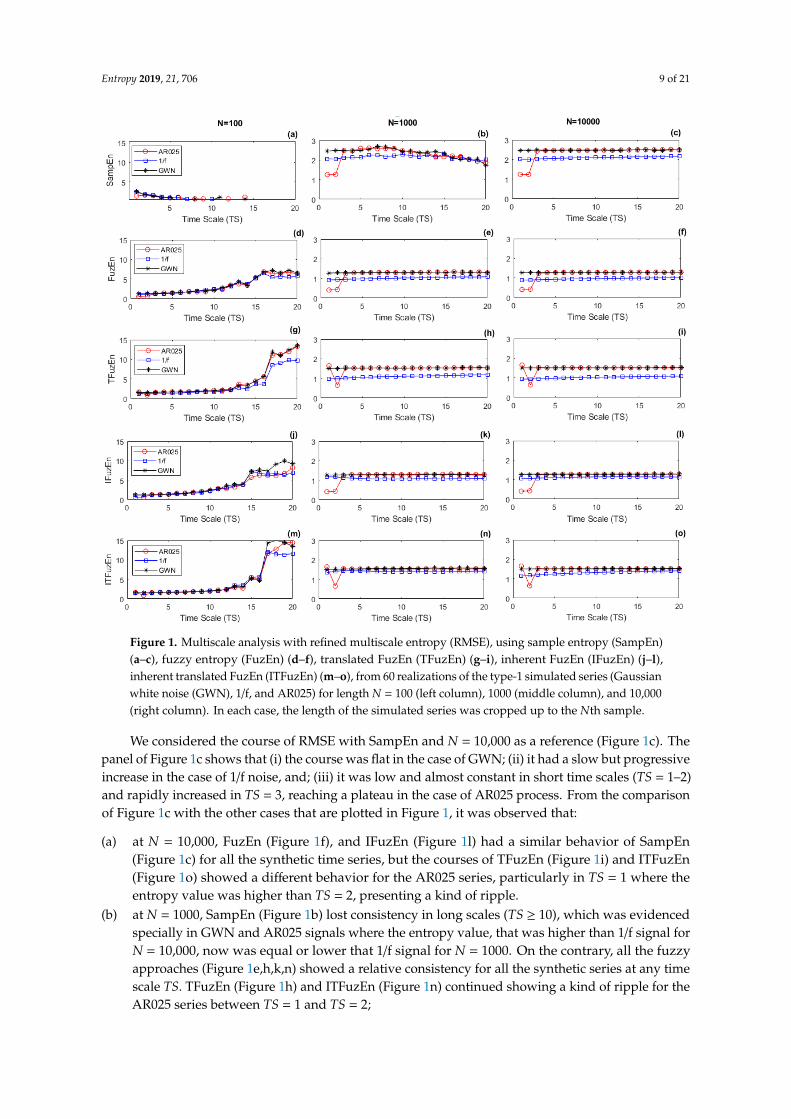
Figure 2 shows, for N = 100, 1000, and 10,000, the course of RMSE approaches as a function of 𝑇𝑆 derived from the 30 realizations of the type-2 synthetic series: Logistic Map with 𝑎 = 3.5 (LM-3.5, blue line with asterisk marker), 𝑎 = 3.7 (LM-3.7, pink line with circle marker), 𝑎 = 3.9 (LM-3.9, black line with diamond marker), and Henon Map with 𝛼 = 1.4 and 𝛽 = 0.3 (HM, red line with square marker).

Figure 1. Multiscale analysis with refined multiscale entropy (RMSE), using sample entropy (SampEn)(a–c), fuzzy entropy (FuzEn) (d–f), translated FuzEn (TFuzEn) (g–i), inherent FuzEn (IFuzEn) (j–l),inherent translated FuzEn (ITFuzEn) (m–o), from 60 realizations of the type-1 simulated series (Gaussianwhite noise (GWN), 1/f, and AR025) for length N = 100 (left column), 1000 (middle column), and 10,000(right column). In each case, the length of the simulated series was cropped up to the Nth sample.

We considered the course of RMSE with SampEn and N = 10,000 as a reference (Figure 1c). Thepanel of Figure 1c shows that (i) the course was flat in the case of GWN; (ii) it had a slow but progressiveincrease in the case of 1/f noise, and; (iii) it was low and almost constant in short time scales (TS = 1–2)and rapidly increased in TS = 3, reaching a plateau in the case of AR025 process. From the comparisonof Figure 1c with the other cases that are plotted in Figure 1, it was observed that:

(a) at N = 10,000, FuzEn (Figure 1f), and IFuzEn (Figure 1l) had a similar behavior of SampEn(Figure 1c) for all the synthetic time series, but the courses of TFuzEn (Figure 1i) and ITFuzEn(Figure 1o) showed a different behavior for the AR025 series, particularly in TS = 1 where theentropy value was higher than TS = 2, presenting a kind of ripple.

(b) at N = 1000, SampEn (Figure 1b) lost consistency in long scales (TS ≥ 10), which was evidencedspecially in GWN and AR025 signals where the entropy value, that was higher than 1/f signal forN = 10,000, now was equal or lower that 1/f signal for N = 1000. On the contrary, all the fuzzyapproaches (Figure 1e,h,k,n) showed a relative consistency for all the synthetic series at any timescale TS. TFuzEn (Figure 1h) and ITFuzEn (Figure 1n) continued showing a kind of ripple for theAR025 series between TS = 1 and TS = 2;

Entropy 2019, 21, 706 10 of 21

(c) at N = 100, all the RMSE metrics lost consistency. Although SampEn values (Figure 1a) could notbe obtained for time scales TS ≥ 7 (short series with less than 14 samples), all the fuzzy approachescould be computed for TS values between 1 and 20.

Figure 2 shows, for N = 100, 1000, and 10,000, the course of RMSE approaches as a function of TSderived from the 30 realizations of the type-2 synthetic series: Logistic Map with a = 3.5 (LM-3.5, blueline with asterisk marker), a = 3.7 (LM-3.7, pink line with circle marker), a = 3.9 (LM-3.9, black linewith diamond marker), and Henon Map with α = 1.4 and β = 0.3 (HM, red line with square marker).Entropy 2019, 21, 706 10 of 20

Figure 2. Multiscale analysis with RMSE, using SampEn (a)–(c), FuzEn (d)–(e), TFuzEn (g)–(i), anslated-reflected FuzEn (TRFuzEn) (j)–(l), IFuzEn (m)–(o), and ITFuzEn (p)–(r), from 30 realizations of the type-2 simulated series (LM-3.5, LM-3.7, LM-3.9, and Henon map (HM)) for length N = 100 (left column), 1000 (middle column), and 10,000 (right column).

We considered the course of RMSE with SampEn and N = 10,000 as a reference (Figure 2c). The panel of Figure 2c shows that (i) the course was flat at zero value for the LM-3.5 signal, which corresponds to the Logistic map in oscillation condition (totally predictable signal) and, therefore, it was expected to have a low value of entropy; (ii) the course exhibited an initial increase at short time scales (1 ≤ TS ≤ 7) and reached a plateau at long time scales for LM-3.7, LM-3.9, and HM signal, which are signals belonging to Logistic and Henon maps in chaotic conditions. From the comparison of Figure 2c with the other cases that are plotted in Figure 2, it was observed that:

(a) at N = 10,000: (i) although all the fuzzy approaches (Figure 2f,i,l,o,r) had a similar behavior of SampEn (Figure 2c) for the chaotic series (LM-3.7, LM-3.9, and HM signals), i.e., the courses exhibited an initial increase and then reached a plateau, the entropy values were lower and with smaller span than SampEn; (ii) only FuzEn (Figure 2f) had a similar behavior than SampEn in the totally predictable signal (LM-3.5); (iii) the course for LM-3.5 showed ripples in TFuzEn (Figure 2i), TRFuzEn (Figure 2l), IFuzEn (Figure 2o) and ITFuzEn (Figure 2r), being TRFuzEn the one with the most prominent ripple;

Figure 2. Multiscale analysis with RMSE, using SampEn (a–c), FuzEn (d–e), TFuzEn (g–i),anslated-reflected FuzEn (TRFuzEn) (j–l), IFuzEn (m–o), and ITFuzEn (p–r), from 30 realizationsof the type-2 simulated series (LM-3.5, LM-3.7, LM-3.9, and Henon map (HM)) for length N = 100 (leftcolumn), 1000 (middle column), and 10,000 (right column).

We considered the course of RMSE with SampEn and N = 10,000 as a reference (Figure 2c).The panel of Figure 2c shows that (i) the course was flat at zero value for the LM-3.5 signal, whichcorresponds to the Logistic map in oscillation condition (totally predictable signal) and, therefore, itwas expected to have a low value of entropy; (ii) the course exhibited an initial increase at short timescales (1 ≤ TS ≤ 7) and reached a plateau at long time scales for LM-3.7, LM-3.9, and HM signal, which

Entropy 2019, 21, 706 11 of 21

are signals belonging to Logistic and Henon maps in chaotic conditions. From the comparison ofFigure 2c with the other cases that are plotted in Figure 2, it was observed that:

(a) at N = 10,000: (i) although all the fuzzy approaches (Figure 2f,i,l,o,r) had a similar behavior ofSampEn (Figure 2c) for the chaotic series (LM-3.7, LM-3.9, and HM signals), i.e., the coursesexhibited an initial increase and then reached a plateau, the entropy values were lower and withsmaller span than SampEn; (ii) only FuzEn (Figure 2f) had a similar behavior than SampEn inthe totally predictable signal (LM-3.5); (iii) the course for LM-3.5 showed ripples in TFuzEn(Figure 2i), TRFuzEn (Figure 2l), IFuzEn (Figure 2o) and ITFuzEn (Figure 2r), being TRFuzEn theone with the most prominent ripple;

(b) at N = 1000: (i) SampEn (Figure 2b) lost consistency in long scales (TS ≥ 10), which was evidencedspecially in the LM-3.9 signal where the entropy value, that was higher or equal than the othersignals for N = 10,000, now was lower than LM-3.7 and HM signals at long scales for N = 1000;(ii) all the fuzzy approaches (Figure 2e,h,k,n,q) showed a relative consistency for all the syntheticseries at any time scale TS; (iii) only SampEn and FuzEn (Figure 2e) showed zero value for LM-3.5in all the time scales; (iv) TFuzEn (Figure 2h), TRFuzEn (Figure 2k), IFuzEn (Figure 2n), andITFuzEn (Figure 2q) continued showing a ripple in the course of LM-3.5;

(c) at N = 100: (i) entropy values decreased in long time scales for SampEn (Figure 2a), while entropyvalues in fuzzy approaches tended to increase in long time scales; (ii) only SampEn and FuzEn(Figure 2d) showed a zero value for LM-3.5 in all the time scales; (iii) SampEn values could not beobtained for time scales TS > 4 (short series with less than 25 samples) in LM-3.9 and for TS > 10for the other series, but all the fuzzy approaches could be computed for all the TS values.

3.2. RMSE of EEG Signals

Firstly, N = 6400, r = 0.15 × SD and m = 2 were taken as fixed parameters in SampEn andFuzEn approaches, in order to compare the prediction probability (Pk values) of the RMSE metricsfor nociception assessment, using EEG signals (Figures 3–5). Secondly, the tolerance parameter r wasvaried between 0.10 and 0.30, in steps of 0.05, to evaluate how this parameter affects the performanceof RMSE metrics in the nociception assessment (Figure 6).

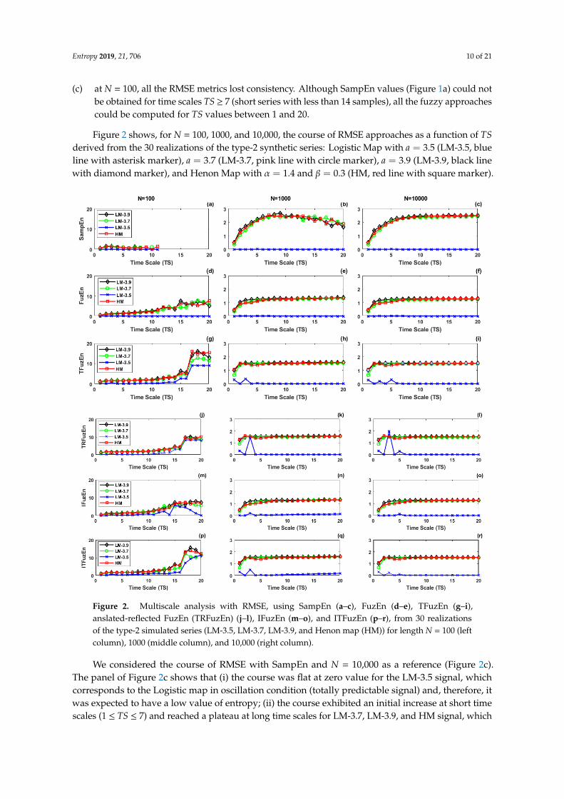
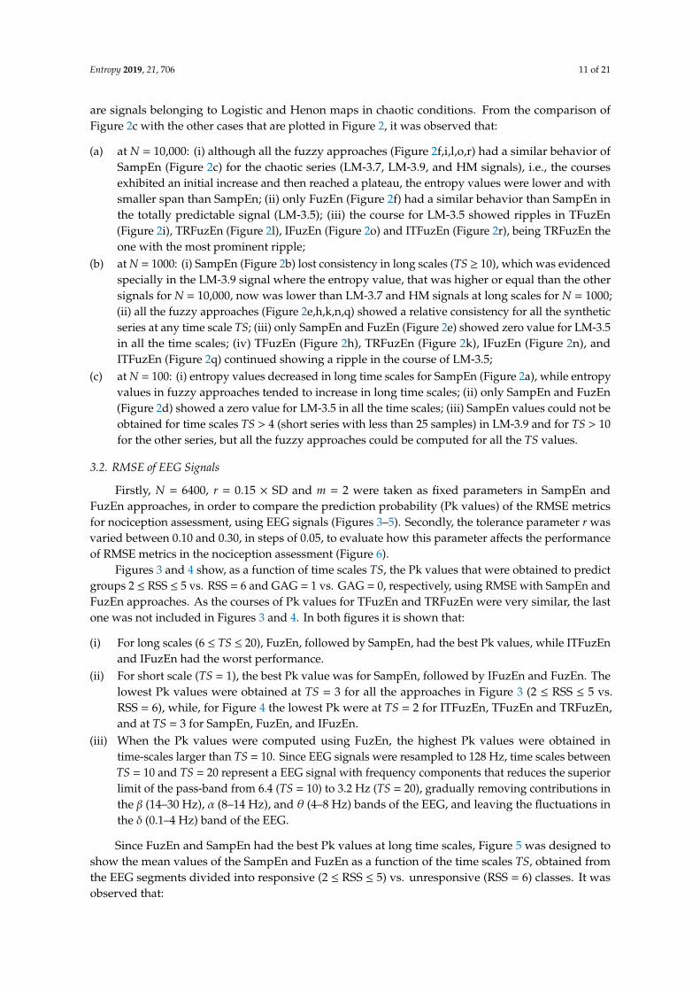
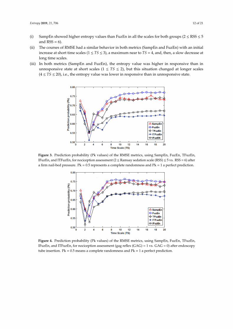
Figures 3 and 4 show, as a function of time scales TS, the Pk values that were obtained to predictgroups 2 ≤ RSS ≤ 5 vs. RSS = 6 and GAG = 1 vs. GAG = 0, respectively, using RMSE with SampEn andFuzEn approaches. As the courses of Pk values for TFuzEn and TRFuzEn were very similar, the lastone was not included in Figures 3 and 4. In both figures it is shown that:

(i) For long scales (6 ≤ TS ≤ 20), FuzEn, followed by SampEn, had the best Pk values, while ITFuzEnand IFuzEn had the worst performance.

(ii) For short scale (TS = 1), the best Pk value was for SampEn, followed by IFuzEn and FuzEn. Thelowest Pk values were obtained at TS = 3 for all the approaches in Figure 3 (2 ≤ RSS ≤ 5 vs.RSS = 6), while, for Figure 4 the lowest Pk were at TS = 2 for ITFuzEn, TFuzEn and TRFuzEn,and at TS = 3 for SampEn, FuzEn, and IFuzEn.

(iii) When the Pk values were computed using FuzEn, the highest Pk values were obtained intime-scales larger than TS = 10. Since EEG signals were resampled to 128 Hz, time scales betweenTS = 10 and TS = 20 represent a EEG signal with frequency components that reduces the superiorlimit of the pass-band from 6.4 (TS = 10) to 3.2 Hz (TS = 20), gradually removing contributions inthe β (14–30 Hz), α (8–14 Hz), and θ (4–8 Hz) bands of the EEG, and leaving the fluctuations inthe δ (0.1–4 Hz) band of the EEG.

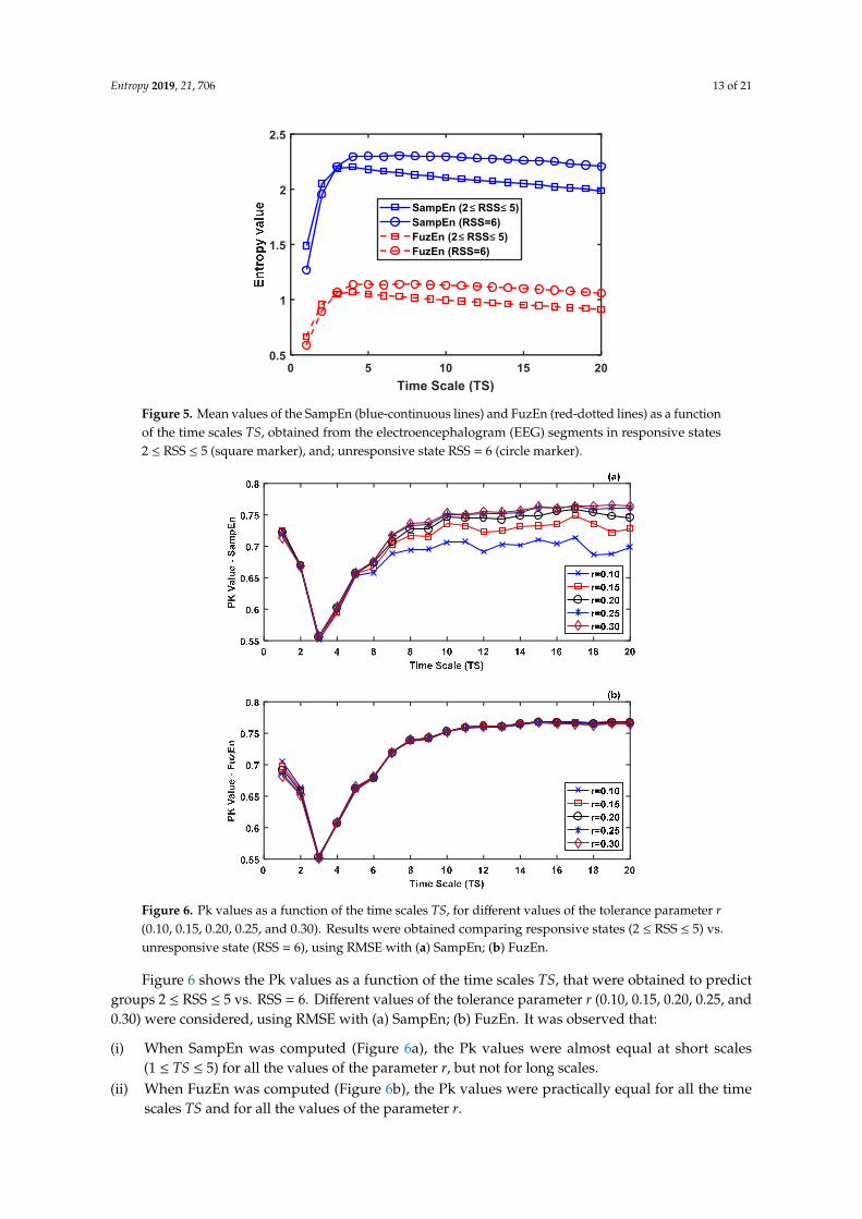
Since FuzEn and SampEn had the best Pk values at long time scales, Figure 5 was designed toshow the mean values of the SampEn and FuzEn as a function of the time scales TS, obtained fromthe EEG segments divided into responsive (2 ≤ RSS ≤ 5) vs. unresponsive (RSS = 6) classes. It wasobserved that:

Entropy 2019, 21, 706 12 of 21

(i) SampEn showed higher entropy values than FuzEn in all the scales for both groups (2 ≤ RSS ≤ 5and RSS = 6).

(ii) The courses of RMSE had a similar behavior in both metrics (SampEn and FuzEn) with an initialincrease at short time scales (1 ≤ TS ≤ 3), a maximum near to TS = 4, and, then, a slow decrease atlong time scales.

(iii) In both metrics (SampEn and FuzEn), the entropy value was higher in responsive than inunresponsive state at short scales (1 ≤ TS ≤ 2), but this situation changed at longer scales(4 ≤ TS ≤ 20), i.e., the entropy value was lower in responsive than in unresponsive state.

Entropy 2019, 21, 706 11 of 20

(b) at N = 1000: (i) SampEn (Figure 2b) lost consistency in long scales (TS >= 10), which was evidenced specially in the LM-3.9 signal where the entropy value, that was higher or equal than the other signals for N = 10,000, now was lower than LM-3.7 and HM signals at long scales for N = 1000; (ii) all the fuzzy approaches (Figure 2e,h,k,n,q) showed a relative consistency for all the synthetic series at any time scale TS; (iii) only SampEn and FuzEn (Figure 2e) showed zero value for LM-3.5 in all the time scales; (iv) TFuzEn (Figure 2h), TRFuzEn (Figure 2k), IFuzEn (Figure 2n), and ITFuzEn (Figure 2q) continued showing a ripple in the course of LM-3.5;

(c) at N = 100: (i) entropy values decreased in long time scales for SampEn (Figure 2a), while entropy values in fuzzy approaches tended to increase in long time scales; (ii) only SampEn and FuzEn (Figure 2d) showed a zero value for LM-3.5 in all the time scales; (iii) SampEn values could not be obtained for time scales TS > 4 (short series with less than 25 samples) in LM-3.9 and for TS > 10 for the other series, but all the fuzzy approaches could be computed for all the TS values.

3.2 RMSE of EEG Signals

Firstly, N = 6400, r = 0.15 × SD and m = 2 were taken as fixed parameters in SampEn and FuzEn approaches, in order to compare the prediction probability (Pk values) of the RMSE metrics for nociception assessment, using EEG signals (Figures 3–5). Secondly, the tolerance parameter r was varied between 0.10 and 0.30, in steps of 0.05, to evaluate how this parameter affects the performance of RMSE metrics in the nociception assessment (Figure 6).

Figures 3 and 4 show, as a function of time scales TS, the Pk values that were obtained to predict groups 2 ≤ RSS ≤ 5 vs. RSS = 6 and GAG = 1 vs. GAG = 0, respectively, using RMSE with SampEn and FuzEn approaches. As the courses of Pk values for TFuzEn and TRFuzEn were very similar, the last one was not included in Figures 3 and 4. In both figures it is shown that:

(i) For long scales (6 ≤ TS ≤ 20), FuzEn, followed by SampEn, had the best Pk values, while ITFuzEn and IFuzEn had the worst performance. (ii) For short scale (TS = 1), the best Pk value was for SampEn, followed by IFuzEn and FuzEn. The lowest Pk values were obtained at TS = 3 for all the approaches in Figure 3 (2 ≤ RSS ≤ 5 vs. RSS = 6), while, for Figure 4 the lowest Pk were at TS = 2 for ITFuzEn, TFuzEn and TRFuzEn, and at TS = 3 for SampEn, FuzEn, and IFuzEn. (iii) When the Pk values were computed using FuzEn, the highest Pk values were obtained in time-scales larger than TS = 10. Since EEG signals were resampled to 128 Hz, time scales between TS = 10 and TS = 20 represent a EEG signal with frequency components that reduces the superior limit of the pass-band from 6.4 (TS = 10) to 3.2 Hz (TS = 20), gradually removing contributions in the 𝛽 (14–30 Hz), 𝛼 (8–14 Hz), and 𝜃 (4–8 Hz) bands of the EEG, and leaving the fluctuations in the 𝛿 (0.1–4 Hz) band of the EEG.

Figure 3. Prediction probability (Pk values) of the RMSE metrics, using SampEn, FuzEn, TFuzEn, IFuzEn, and ITFuzEn, for nociception assessment (2 ≤ Ramsay sedation scale (RSS) ≤ 5 vs. RSS = 6)

Figure 3. Prediction probability (Pk values) of the RMSE metrics, using SampEn, FuzEn, TFuzEn,IFuzEn, and ITFuzEn, for nociception assessment (2 ≤ Ramsay sedation scale (RSS) ≤ 5 vs. RSS = 6) aftera firm nail-bed pressure. Pk = 0.5 represents a complete randomness and Pk = 1 a perfect prediction.

Entropy 2019, 21, 706 12 of 20

after a firm nail-bed pressure. Pk = 0.5 represents a complete randomness and Pk = 1 a perfect prediction.

Figure 4. Prediction probability (Pk values) of the RMSE metrics, using SampEn, FuzEn, TFuzEn, IFuzEn, and ITFuzEn, for nociception assessment (gag reflex (GAG) = 1 vs. GAG = 0) after endoscopy tube insertion. Pk = 0.5 means a complete randomness and Pk = 1 a perfect prediction.

Since FuzEn and SampEn had the best Pk values at long time scales, Figure 5 was designed to show the mean values of the SampEn and FuzEn as a function of the time scales TS, obtained from the EEG segments divided into responsive (2 ≤ RSS ≤ 5) vs. unresponsive (RSS = 6) classes. It was observed that:

(i) SampEn showed higher entropy values than FuzEn in all the scales for both groups (2 ≤ RSS ≤ 5 and RSS = 6). (ii) The courses of RMSE had a similar behavior in both metrics (SampEn and FuzEn) with an initial increase at short time scales (1 ≤ TS ≤ 3), a maximum near to TS = 4, and, then, a slow decrease at long time scales. (iii) In both metrics (SampEn and FuzEn), the entropy value was higher in responsive than in unresponsive state at short scales (1 ≤ TS ≤ 2), but this situation changed at longer scales (4 ≤ TS ≤ 20), i.e., the entropy value was lower in responsive than in unresponsive state.

Figure 5. Mean values of the SampEn (blue-continuous lines) and FuzEn (red-dotted lines) as a function of the time scales TS, obtained from the electroencephalogram (EEG) segments in responsive states 2 ≤ RSS ≤ 5 (square marker), and; unresponsive state RSS = 6 (circle marker).

0 5 10 15 20Time Scale (TS)

0.5

1

1.5

2

2.5

SampEn (2≤ RSS≤ 5)SampEn (RSS=6)FuzEn (2≤ RSS≤ 5)FuzEn (RSS=6)

Figure 4. Prediction probability (Pk values) of the RMSE metrics, using SampEn, FuzEn, TFuzEn,IFuzEn, and ITFuzEn, for nociception assessment (gag reflex (GAG) = 1 vs. GAG = 0) after endoscopytube insertion. Pk = 0.5 means a complete randomness and Pk = 1 a perfect prediction.

Entropy 2019, 21, 706 13 of 21

Entropy 2019, 21, 706 12 of 20

after a firm nail-bed pressure. Pk = 0.5 represents a complete randomness and Pk = 1 a perfect prediction.

Figure 4. Prediction probability (Pk values) of the RMSE metrics, using SampEn, FuzEn, TFuzEn, IFuzEn, and ITFuzEn, for nociception assessment (gag reflex (GAG) = 1 vs. GAG = 0) after endoscopy tube insertion. Pk = 0.5 means a complete randomness and Pk = 1 a perfect prediction.

Since FuzEn and SampEn had the best Pk values at long time scales, Figure 5 was designed to show the mean values of the SampEn and FuzEn as a function of the time scales TS, obtained from the EEG segments divided into responsive (2 ≤ RSS ≤ 5) vs. unresponsive (RSS = 6) classes. It was observed that:

(i) SampEn showed higher entropy values than FuzEn in all the scales for both groups (2 ≤ RSS ≤ 5 and RSS = 6). (ii) The courses of RMSE had a similar behavior in both metrics (SampEn and FuzEn) with an initial increase at short time scales (1 ≤ TS ≤ 3), a maximum near to TS = 4, and, then, a slow decrease at long time scales. (iii) In both metrics (SampEn and FuzEn), the entropy value was higher in responsive than in unresponsive state at short scales (1 ≤ TS ≤ 2), but this situation changed at longer scales (4 ≤ TS ≤ 20), i.e., the entropy value was lower in responsive than in unresponsive state.

Figure 5. Mean values of the SampEn (blue-continuous lines) and FuzEn (red-dotted lines) as a function of the time scales TS, obtained from the electroencephalogram (EEG) segments in responsive states 2 ≤ RSS ≤ 5 (square marker), and; unresponsive state RSS = 6 (circle marker).

0 5 10 15 20Time Scale (TS)

0.5

1

1.5

2

2.5

SampEn (2≤ RSS≤ 5)SampEn (RSS=6)FuzEn (2≤ RSS≤ 5)FuzEn (RSS=6)

Figure 5. Mean values of the SampEn (blue-continuous lines) and FuzEn (red-dotted lines) as a functionof the time scales TS, obtained from the electroencephalogram (EEG) segments in responsive states2 ≤ RSS ≤ 5 (square marker), and; unresponsive state RSS = 6 (circle marker).

Entropy 2019, 21, 706 13 of 20

Figure 6 shows the Pk values as a function of the time scales TS, that were obtained to predict groups 2 ≤ RSS ≤ 5 vs. RSS = 6. Different values of the tolerance parameter r (0.10, 0.15, 0.20, 0.25, and 0.30) were considered, using RMSE with (a) SampEn; (b) FuzEn. It was observed that:

(i) When SampEn was computed (Figure 6a), the Pk values were almost equal at short scales (1 ≤ TS ≤ 5) for all the values of the parameter r, but not for long scales. (ii) When FuzEn was computed (Figure 6b), the Pk values were practically equal for all the time scales TS and for all the values of the parameter r. (iii) The best Pk values were obtained for long scales in both RMSE using SampEn and using FuzEn.

Figure 6. Pk values as a function of the time scales TS, for different values of the tolerance parameter r (0.10, 0.15, 0.20, 0.25, and 0.30). Results were obtained comparing responsive states (2 ≤ RSS ≤ 5) vs. unresponsive state (RSS = 6), using RMSE with (a) SampEn; (b) FuzEn.

4. Discussion

In previous works [1,2], FuzEn has been proposed as an entropy measure that is more consistent and less dependent on the data length than SampEn, and several variants have been designed to further improve FuzEn performance over short time series. Indeed, approaches as TFuzEn, TRFuzEn, IFuzEn, and ITFuzEn have been introduced [9,10] to increase the number of patterns that are compared without changing the length of the time series and limiting the effect of local variation of the mean. In the present work, these metrics were included in a multiscale analysis, using RMSE applied to signals with different characteristics (fully stochastic, stochastic with long-range correlation, stochastic with some deterministic parts and thus partially predictable, totally predictable, chaotic and real EEG signals). The study was mainly focused to compare the performance of RMSE, with SampEn and FuzEn approaches, as a function of the length of the data and the type of the series. Additionally, metrics were compared according to the prediction probability value (Pk) of pain response in patients under sedation-analgesia, while varying the tolerance parameter r.

In relation with long data series (N = 10,000), the results showed that the course of RMSE had the same tendency with FuzEn approaches as with SampEn, when they were applied to signals with the following behavior (Figures 1 and 2): fully stochastic (GWN), stochastic with long-range

Figure 6. Pk values as a function of the time scales TS, for different values of the tolerance parameter r(0.10, 0.15, 0.20, 0.25, and 0.30). Results were obtained comparing responsive states (2 ≤ RSS ≤ 5) vs.unresponsive state (RSS = 6), using RMSE with (a) SampEn; (b) FuzEn.

Figure 6 shows the Pk values as a function of the time scales TS, that were obtained to predictgroups 2 ≤ RSS ≤ 5 vs. RSS = 6. Different values of the tolerance parameter r (0.10, 0.15, 0.20, 0.25, and0.30) were considered, using RMSE with (a) SampEn; (b) FuzEn. It was observed that:

(i) When SampEn was computed (Figure 6a), the Pk values were almost equal at short scales(1 ≤ TS ≤ 5) for all the values of the parameter r, but not for long scales.

(ii) When FuzEn was computed (Figure 6b), the Pk values were practically equal for all the timescales TS and for all the values of the parameter r.

Entropy 2019, 21, 706 14 of 21

(iii) The best Pk values were obtained for long scales in both RMSE using SampEn and using FuzEn.

4. Discussion

In previous works [1,2], FuzEn has been proposed as an entropy measure that is more consistentand less dependent on the data length than SampEn, and several variants have been designed tofurther improve FuzEn performance over short time series. Indeed, approaches as TFuzEn, TRFuzEn,IFuzEn, and ITFuzEn have been introduced [9,10] to increase the number of patterns that are comparedwithout changing the length of the time series and limiting the effect of local variation of the mean.In the present work, these metrics were included in a multiscale analysis, using RMSE applied tosignals with different characteristics (fully stochastic, stochastic with long-range correlation, stochasticwith some deterministic parts and thus partially predictable, totally predictable, chaotic and real EEGsignals). The study was mainly focused to compare the performance of RMSE, with SampEn andFuzEn approaches, as a function of the length of the data and the type of the series. Additionally,metrics were compared according to the prediction probability value (Pk) of pain response in patientsunder sedation-analgesia, while varying the tolerance parameter r.

In relation with long data series (N = 10,000), the results showed that the course of RMSE had thesame tendency with FuzEn approaches as with SampEn, when they were applied to signals with thefollowing behavior (Figures 1 and 2): fully stochastic (GWN), stochastic with long-range correlation(1/f), and chaotic (LM-3.7, LM-3.9, and HM). However, there were important differences between someof the RMSE courses obtained from partially predictable (AR025) and totally predictable (LM-3.5)signals. The more relevant case was the one related to the totally predictable (LM-3.5) signal. LM-3.5is a periodic signal with a deterministic behavior, which should have a very low entropy rate valueresulting from its periodic nature that does not generate new information. However, all the FuzEnvariants, with the exception of FuzEn, showed ripples with values different from zero in this typeof signal. This suggests that metrics such as TFuzEn, TRFuzEn, IFuzEn, and ITFuzEn introducesome kind of irregularity with different levels of predictability, especially in the longer time scales.Approaches as TRFuzEn and ITFuzEn are based on TFuzEn [9], so that all of them remove the meanvalue of m-dimensional patterns before computing the probability of finding matched patterns, thussuggesting that removing the mean over patterns might be responsible for the introduction of somedegree of randomness.

Comparing the performance of RMSE courses as a function of the series length N, SampEn metriclost consistency using series with length N = 1000 in comparison to series of length N = 10,000. On thecontrary, all the fuzzy approaches showed a relative consistency for all the synthetic series at any timescale TS, demonstrating to be less dependent on the data length as it was indicated in [1,2]. The loss ofconsistency in SampEn was more evident for long scales (TS ≥ 10), where the series has reduced itslength to N/TS = 1000/10 = 100 samples or less. This result is in agreement with [21], where it wasreported the dependence of SampEn with the series length and how this metric loses consistency whendata length is smaller than 300.

The analysis with series of length N = 100 allowed the performance of RMSE metrics in shorttime series to be evaluated. Although all the metrics lost consistency compared to series with lengthN = 10,000, the most relevant finding was that, while SampEn values could not be obtained for longtime scales, fuzzy approaches could be computed for all the TS values (from 1 to 20). For example,in this study, SampEn could not be computed for short series with less than 25 samples in LM-3.9signals. By its definition, SampEn depends of the logarithm of the ratio (Am

r /Bmr ), and this logarithm

is indeterminate if there are not patterns that match for m and m + 1 samples at the same time. Thiscondition is minimized in Fuzzy entropy definition and in its variants that increment the number ofpatterns that are compared without changing the length of the time series, allowing the computationof the metrics even in very short series.

About the nociception assessment using EEG signals for classifying RSS values and GAG responses(2≤RSS≤ 5 vs. RSS = 6 and GAG = 1 vs. GAG = 0 in Figures 3 and 4, respectively), the best performance

Entropy 2019, 21, 706 15 of 21

was obtained with FuzEn, followed by SampEn, in middle and long scales. These results suggest thatalthough the variants of FuzEn are metrics less dependent on the data length, this does not meanthat they provide an estimate of conditional probability better than SampEn or FuzEn. The methodsused for these metrics to create new patterns increase the probability of finding similar patterns, thusincreasing the regularity of the series and reducing conditional entropy, and this attitude reducesthe possibility to differentiate nociceptive states. Considering that the procedure to compute RMSEreduces the time series length as a function of TS, the best Pk values that were obtained with FuzEncan be related with the fact that FuzEn was more consistent and less dependent on the data length thanSampEn. On the other hand, ITFuzEn and IFuzEn had the worst performance in middle and longscales. These two approaches are based on the EMD as a method to reduce superimposed trends intime series, in order to moderate the effect of trends in the increment of the standard deviation of thedata. However, this procedure seems to worsen the performance of RMSE in middle and long scales incomparison with approaches that do not eliminate the trends as SampEn. This can be related with thefact that RMSE adjusts the tolerance for comparing patterns as function of the standard deviation ofeach the time series, thus limiting the dependence of RMSE on the reduction of variance due to theelimination of the fast temporal scales [11].

In relation to the results of RMSE obtained from the EEG segments when they were divided intoresponsive (2 ≤ RSS ≤ 5) and unresponsive (RSS = 6) classes (Figure 5), we conclude that (i) the lowervalues of FuzEn compared to SampEn are linked to the fact that the fuzzy membership functionsincreases the probability of finding similar patterns that match for m and m + 1 samples at the sametime, thus increasing the regularity in the series; (ii) the regularity of the EEG signal was higher atshort time scales (TS < 3) than in long time scales, which indicates that the lower frequency bands as α,θ and δ contain the more complex activity of the EEG in those patients; (iii) the complexity of the EEGsegments relevant to the responsive class was higher at short time scales (TS = 1) and lower at longtime scales than those relevant to the unresponsive class. As was discussed in [15], the scalp and facialmuscle activity, in patients of the responsive group (patients with low sedation level), is associated tothe higher complexity of the EEG in short time scales and to a greater probability of feel pain thanthe unresponsive group. At long time scales, the higher complexity in unresponsive group (patientswith higher sedation level than the responsive group) is associated with the displacement of the EEGactivity to low frequency bands as the level of sedation increases.

The impact of the tolerance parameter r, used to determine the similarity between patterns inSampEn and FuzEn, on the Pk statistic was evaluated. Indeed, the Pk was computed for differentvalues of r, between r = 0.10 and 0.30, for each one of the RMSE metrics as a function of the TS, inrelation to the ability of predicting responsive (2 ≤ RSS ≤ 5) and unresponsive (RSS = 6) subjects. Atlong time scales, RMSE with SampEn showed important variations in the Pk statistic for different rvalues at the same TS, while the Pk was practically equal in FuzEn for all the r values at the sameTS. This multiscale analysis evidenced the low dependence of FuzEn with the value of the toleranceparameter r, in comparison with SampEn. As was pointed out in [1,2], the Heaviside function used bySampEn creates a rigid boundary that can lead to sudden variations of the entropy values when thetolerance parameter r varies. As a result, SampEn may rise or fall dramatically when the tolerance r isslightly changed. Conversely, FuzEn employs an exponential function with soft boundaries, in such away that entropy values are more stables to changes in r.

5. Conclusions

This work validated the RMSE performance when FuzEn, with different refinements, wasimplemented instead of SampEn for computing the entropy-based measure. Indeed, SampEn, FuzEn,TFuzEn, TRFuzEn, IFuzEn, and ITFuzEn were applied at different time scales to synthetic andexperimental time series. The results of the present study suggest that it is necessary to be cautiouswith the application of some FuzEn variants, and with the interpretation of their findings. Indeed,approaches based on the elimination of the mean value of the patterns before computing the probability

Entropy 2019, 21, 706 16 of 21

of finding matches (TFuzEn, TRFuzEn, and ITFuzEn) showed high entropy values over predictableprocess that should have low entropy values. Additionally, FuzEn methods using the EMD approachto reduce the effect of superimposed trends in time series (ITFuzEn and IFuzEn) seem to worsen theperformance of RMSE at middle and long scales. In general, FuzEn showed a similar behavior toSampEn in series with long lengths, with the advantage of being more consistent than SampEn overshort-length time series, less dependent on the tolerance parameter r, and stronger in the nociceptionprediction especially at long time scales (6 ≤ TS ≤ 20). Therefore, because of that, FuzEn can be moresuitable in real-time and real-world applications.

Author Contributions: Conceptualization, J.F.V., M.V. and A.P.; methodology, J.F.V. and J.D.B.; software, J.F.V.and J.D.B.; validation, J.D.B.; formal analysis, J.F.V.; M.V. and A.P.; writing—original draft preparation, J.F.V. andJ.D.B.; writing—review and editing, M.V., E.W.J., A.P. and P.L.G.; funding acquisition, J.F.V. and P.L.G.

Funding: This research was funded by COLCIENCIAS, grant number 1232-807-64083 and the UPC member wassupported by MINECO (DPI2017-89827-R) from Spanish Government. CIBER of Bioengineering, Biomaterialsand Nanomedicine, an initiative of ISCIII.

Conflicts of Interest: The authors declare no conflict of interest. The funders had no role in the design of thestudy; in the collection, analyses, or interpretation of data; in the writing of the manuscript, or in the decision topublish the results.

Appendix A Empirical Mode Decomposition (EMD)

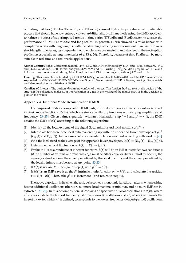
The empirical mode decomposition (EMD) algorithm decomposes a time series into a series ofintrinsic mode functions (IMFs), which are simple oscillatory functions with varying amplitude andfrequency [23–25]. Given a time signal x(t), with an initialization step i = 1 and ρ0 = x(t), the EMDobtains the IMFs of x(t) according to the following algorithm:

(1) Identify all the local extrema of the signal (local minima and local maxima of ρi−1).(2) Interpolate between these local extrema, ending up with the upper and lower envelopes of ρi−1

(Eup(t) and Elow(t)). In this case a cubic spline interpolation was used according with work in [25].(3) Find the local trend as the average of the upper and lower envelopes, Qi(t) = (Eup(t) +Elow(t))/2.(4) Determine the local fluctuation as, h(t) = X(t) −Qi(t).(5) Evaluate h(t) as a candidate of inherent functions; h(t) will be an IMF if it satisfies two conditions:

(i) the number of extrema and zero crossings must be either equal or differ at most by one; (ii) theaverage value between the envelope defined by the local maxima and the envelope defined bythe local minima, must be zero at any point [23,25].

(6) If h(t) is not an IMF, then go to step (1) with ρi−1 = h(t).(7) If h(t) is an IMF, save it as the ith intrinsic mode function mi = h(t), and calculate the residue

r = x(t) − h(t). Then, take ρi = r, increment i, and return to step (1).

The above algorithm halts when the residue becomes a monotonic function, it means, when residuehas no additional oscillations (there are not more local maxima or minima), and no more IMF can beextracted [23–28]. In this decomposition, mi contains a “spectrum” of local oscillations in x(n), wherem1 corresponds to the highest frequency (shortest-period) oscillations and ml, where l represents thelargest index for which mi is defined, corresponds to the lowest frequency (longest-period) oscillations.

Entropy 2019, 21, 706 17 of 21

Entropy 2019, 21, 706 16 of 20

The empirical mode decomposition (EMD) algorithm decomposes a time series into a series of intrinsic mode functions (IMFs), which are simple oscillatory functions with varying amplitude and frequency [23–25]. Given a time signal 𝑥(𝑡), with an initialization step 𝑖 = 1 and 𝜌 = 𝑥(𝑡), the EMD obtains the IMFs of 𝑥(𝑡) according to the following algorithm: (1) Identify all the local extrema of the signal (local minima and local maxima of 𝜌 ). (2) Interpolate between these local extrema, ending up with the upper and lower envelopes of 𝜌

(𝐸 (𝑡) and 𝐸 (𝑡)). In this case a cubic spline interpolation was used according with work in [25].

(3) Find the local trend as the average of the upper and lower envelopes, 𝑄 (𝑡) = (𝐸 (𝑡) +𝐸 (𝑡))/2. (4) Determine the local fluctuation as, ℎ(𝑡) = 𝑋(𝑡) − 𝑄 (𝑡). (5) Evaluate ℎ(𝑡) as a candidate of inherent functions; ℎ(𝑡) will be an IMF if it satisfies two

conditions: (i) the number of extrema and zero crossings must be either equal or differ at most by one; (ii) the average value between the envelope defined by the local maxima and the envelope defined by the local minima, must be zero at any point [23,25].

(6) If ℎ(𝑡) is not an IMF, then go to step (1) with 𝜌 = ℎ(𝑡). (7) If ℎ(𝑡) is an IMF, save it as the 𝑖 intrinsic mode function 𝑚 = ℎ(𝑡), and calculate the residue 𝑟 = 𝑥(𝑡) − ℎ(𝑡). Then, take 𝜌 = 𝑟, increment 𝑖, and return to step (1).

The above algorithm halts when the residue becomes a monotonic function, it means, when residue has no additional oscillations (there are not more local maxima or minima), and no more IMF can be extracted [23–28]. In this decomposition, 𝑚 contains a ‘‘spectrum’’ of local oscillations in 𝑥(𝑛) , where 𝑚 corresponds to the highest frequency (shortest-period) oscillations and 𝑚 , where 𝑙 represents the largest index for which 𝑚 is defined, corresponds to the lowest frequency (longest-period) oscillations.

Figure A1. Empirical mode decomposition (EMD) results on a sinusoidal input signal with five frequency components: 10, 50, 100, 300, and 500 Hz, with an amplitude of 30, 10, 1, 20 and 5, respectively.

Figure A1. Empirical mode decomposition (EMD) results on a sinusoidal input signal with fivefrequency components: 10, 50, 100, 300, and 500 Hz, with an amplitude of 30, 10, 1, 20 and 5, respectively.

Figure A1 shows the EMD results on a sinusoidal input signal with five frequency components:10, 50, 100, 300, and 500 Hz, with an amplitude of 30, 10, 1, 20 and 5, respectively.

If we sum all IMFs and residue, we will obtain the original input signal. This is,

x(n) =

l∑i=1

mi

+ r. (A1)

However, the main purpose of using EMD on our input signal is performing a trend filtering.This can be done choosing the best IMF index i∗ which allows to separate the trend from thefluctuation [25–27]. In the presence of a trend, the IMF index i shows a rupture in two properties; (i) themean frequency of the successive IMFs of broadband processes decrease [24–26]; (ii) the “energy” ofthe IMFs decreases as the index of the IMFs increases [25,27,28]. Taking into account the describedIMFs properties, the authors in [25] carried on a study to determine the best approach to estimate i∗.Results in [25] showed that the best one is the energy-ratio approach. This approach combines theenergy approach and ratio approach in order to reduce the false detections of i∗.

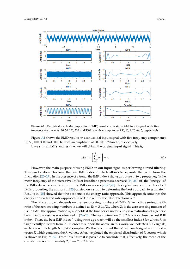
The ratio approach depends on the zero crossing numbers of IMFs. Given a time series, the ithratio of the zero crossing numbers is defined as Ri = Zi−1/Zi, where Zi is the zero crossing number ofits ith IMF. The approximation Ri ≈ 2 holds if the time series under study is a realization of a genericbroadband process, as was observed in [24–26]. The approximation Ri ≈ 2 fails for i close the best IMFindex. Then, the best IMF index i∗ using ratio approach will be the smallest index i for which Ri is“significantly different from 2”. In order to support the above, in this work, we took 2633 EEG signals,each one with a length N = 6400 samples. We then computed the IMFs of each signal and found avector R which contained the Ri values. After, we plotted the empirical distribution of R vectors whichis shown in Figure A2. From this figure it is possible to conclude that, effectively, the mean of thedistribution is approximately 2, then Ri ≈ 2 holds.

Entropy 2019, 21, 706 18 of 21

Entropy 2019, 21, 706 17 of 20

Figure A1 shows the EMD results on a sinusoidal input signal with five frequency components: 10, 50, 100, 300, and 500 Hz, with an amplitude of 30, 10, 1, 20 and 5, respectively.

If we sum all IMFs and residue, we will obtain the original input signal. This is,

𝑥(𝑛) = 𝑚 + 𝑟. (11)

However, the main purpose of using EMD on our input signal is performing a trend filtering. This can be done choosing the best IMF index 𝑖∗ which allows to separate the trend from the fluctuation [25–27]. In the presence of a trend, the IMF index 𝑖 shows a rupture in two properties; (i) the mean frequency of the successive IMFs of broadband processes decrease [24–26]; (ii) the ‘‘energy’’ of the IMFs decreases as the index of the IMFs increases [25,27,28]. Taking into account the described IMFs properties, the authors in [25] carried on a study to determine the best approach to estimate 𝑖∗. Results in [25] showed that the best one is the energy-ratio approach. This approach combines the energy approach and ratio approach in order to reduce the false detections of 𝑖∗.

The ratio approach depends on the zero crossing numbers of IMFs. Given a time series, the 𝑖 ratio of the zero crossing numbers is defined as 𝑅 = 𝑍 /𝑍 , where 𝑍 is the zero crossing number of its 𝑖 IMF. The approximation 𝑅 ≈ 2 holds if the time series under study is a realization of a generic broadband process, as was observed in [24–26]. The approximation 𝑅 ≈ 2 fails for 𝑖 close the best IMF index. Then, the best IMF index 𝑖∗ using ratio approach will be the smallest index 𝑖 for which 𝑅 is ‘‘significantly different from 2’’. In order to support the above, in this work, we took 2633 EEG signals, each one with a length N = 6400 samples. We then computed the IMFs of each signal and found a vector 𝑅 which contained the 𝑅 values. After, we plotted the empirical distribution of R vectors which is shown in Figure A2. From this figure it is possible to conclude that, effectively, the mean of the distribution is approximately 2, then 𝑅 ≈ 2 holds.

Figure A2. Ratio approach: empirical distribution of R vectors of EEG signals used in this work. The vertical red line represents the mean of the distribution of the R vectors (𝑅 ≈ 2). Vertical black lines represent the left and right thresholds using a value of 𝑝 = 15.

The energy approach is based on an empirical property of the so-called ‘‘energy’’ of the IMFs, which can be defined as: 𝐺 = |𝑚 | , 1 ≤ 𝑖 ≤ 𝑙. (12)𝐺 is a decreasing sequence in 𝑖 if the time series under study are realizations of a generic broadband process [27,28]. Thus, the best IMF index 𝑖∗, using energy approach, will be the smallest

Figure A2. Ratio approach: empirical distribution of R vectors of EEG signals used in this work. Thevertical red line represents the mean of the distribution of the R vectors (Ri ≈ 2). Vertical black linesrepresent the left and right thresholds using a value of p = 15.

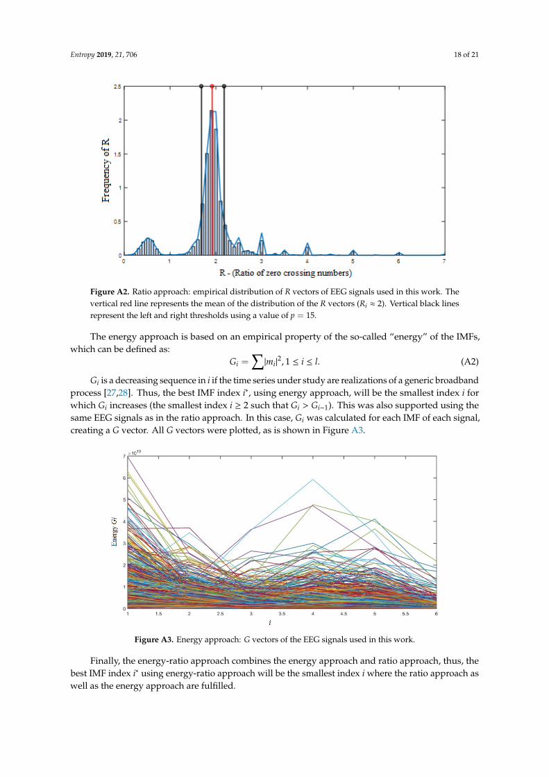
The energy approach is based on an empirical property of the so-called “energy” of the IMFs,which can be defined as:

Gi =∑|mi|

2, 1 ≤ i ≤ l. (A2)

Gi is a decreasing sequence in i if the time series under study are realizations of a generic broadbandprocess [27,28]. Thus, the best IMF index i∗, using energy approach, will be the smallest index i forwhich Gi increases (the smallest index i ≥ 2 such that Gi > Gi−1). This was also supported using thesame EEG signals as in the ratio approach. In this case, Gi was calculated for each IMF of each signal,creating a G vector. All G vectors were plotted, as is shown in Figure A3.

Entropy 2019, 21, 706 18 of 20

index 𝑖 for which 𝐺 increases (the smallest index 𝑖 ≥ 2 such that 𝐺 > 𝐺 ). This was also supported using the same EEG signals as in the ratio approach. In this case, 𝐺 was calculated for each IMF of each signal, creating a 𝐺 vector. All 𝐺 vectors were plotted, as is shown in Figure A3.

Figure A3. Energy approach: 𝐺 vectors of the EEG signals used in this work

Finally, the energy-ratio approach combines the energy approach and ratio approach, thus, the best IMF index 𝑖∗ using energy-ratio approach will be the smallest index 𝑖 where the ratio approach as well as the energy approach are fulfilled.

Therefore, trend 𝑇(𝑡) and fluctuation 𝐹(𝑡) are defined as:

𝑇(𝑡) = 𝑚∗ , (13)

𝐹(𝑡) = 𝑚∗ . (14)

An example of the above is presented in Figure A4.

Figure A4. Trend filtering process applied on a sinusoidal input signal with five frequency components.

Figure A3. Energy approach: G vectors of the EEG signals used in this work.

Finally, the energy-ratio approach combines the energy approach and ratio approach, thus, thebest IMF index i∗ using energy-ratio approach will be the smallest index i where the ratio approach aswell as the energy approach are fulfilled.

Entropy 2019, 21, 706 19 of 21

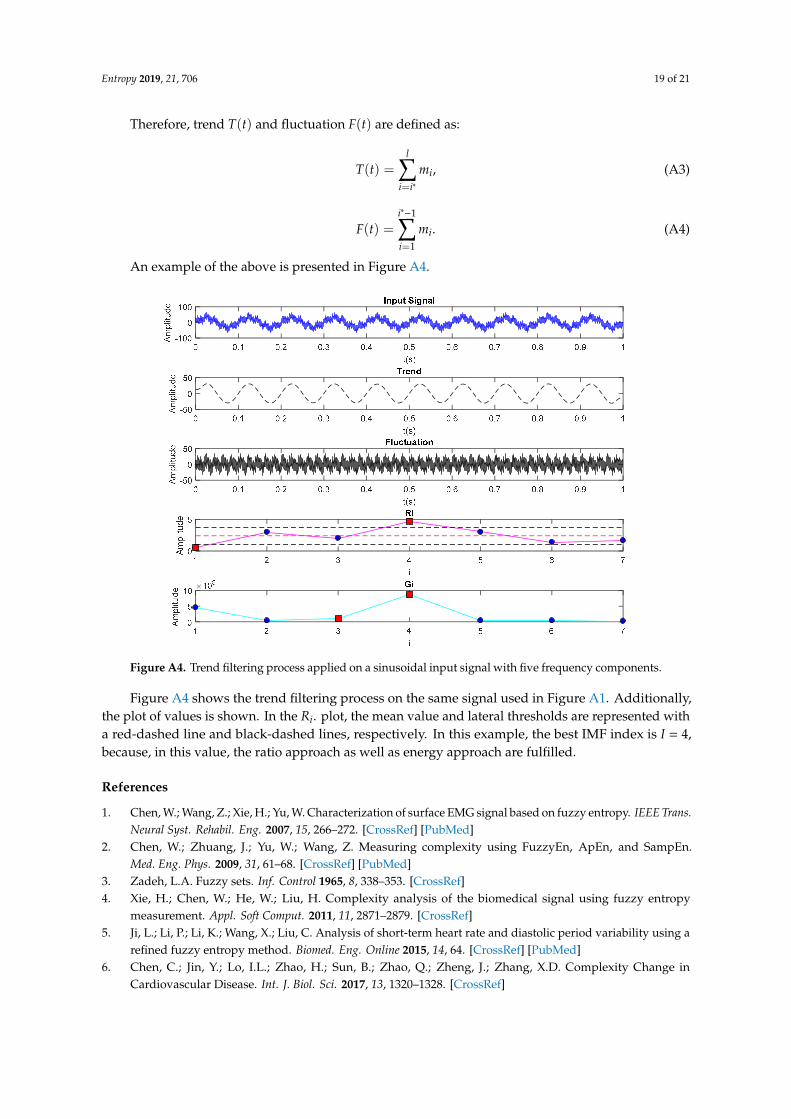
Therefore, trend T(t) and fluctuation F(t) are defined as:

T(t) =l∑

i=i∗mi, (A3)

F(t) =i∗−1∑i=1

mi. (A4)

An example of the above is presented in Figure A4.

Entropy 2019, 21, 706 18 of 20

index 𝑖 for which 𝐺 increases (the smallest index 𝑖 ≥ 2 such that 𝐺 > 𝐺 ). This was also supported using the same EEG signals as in the ratio approach. In this case, 𝐺 was calculated for each IMF of each signal, creating a 𝐺 vector. All 𝐺 vectors were plotted, as is shown in Figure A3.

Figure A3. Energy approach: 𝐺 vectors of the EEG signals used in this work

Finally, the energy-ratio approach combines the energy approach and ratio approach, thus, the best IMF index 𝑖∗ using energy-ratio approach will be the smallest index 𝑖 where the ratio approach as well as the energy approach are fulfilled.

Therefore, trend 𝑇(𝑡) and fluctuation 𝐹(𝑡) are defined as:

𝑇(𝑡) = 𝑚∗ , (13)

𝐹(𝑡) = 𝑚∗ . (14)

An example of the above is presented in Figure A4.

Figure A4. Trend filtering process applied on a sinusoidal input signal with five frequency components.

Figure A4. Trend filtering process applied on a sinusoidal input signal with five frequency components.

Figure A4 shows the trend filtering process on the same signal used in Figure A1. Additionally,the plot of values is shown. In the Ri. plot, the mean value and lateral thresholds are represented witha red-dashed line and black-dashed lines, respectively. In this example, the best IMF index is I = 4,because, in this value, the ratio approach as well as energy approach are fulfilled.

References

1. Chen, W.; Wang, Z.; Xie, H.; Yu, W. Characterization of surface EMG signal based on fuzzy entropy. IEEE Trans.Neural Syst. Rehabil. Eng. 2007, 15, 266–272. [CrossRef] [PubMed]

2. Chen, W.; Zhuang, J.; Yu, W.; Wang, Z. Measuring complexity using FuzzyEn, ApEn, and SampEn.Med. Eng. Phys. 2009, 31, 61–68. [CrossRef] [PubMed]

3. Zadeh, L.A. Fuzzy sets. Inf. Control 1965, 8, 338–353. [CrossRef]4. Xie, H.; Chen, W.; He, W.; Liu, H. Complexity analysis of the biomedical signal using fuzzy entropy

measurement. Appl. Soft Comput. 2011, 11, 2871–2879. [CrossRef]5. Ji, L.; Li, P.; Li, K.; Wang, X.; Liu, C. Analysis of short-term heart rate and diastolic period variability using a

refined fuzzy entropy method. Biomed. Eng. Online 2015, 14, 64. [CrossRef] [PubMed]6. Chen, C.; Jin, Y.; Lo, I.L.; Zhao, H.; Sun, B.; Zhao, Q.; Zheng, J.; Zhang, X.D. Complexity Change in

Cardiovascular Disease. Int. J. Biol. Sci. 2017, 13, 1320–1328. [CrossRef]

Entropy 2019, 21, 706 20 of 21

7. Xie, H.; Guo, T. Fuzzy entropy spectrum analysis for biomedical signals de-noising. In Proceedings ofthe 2018 IEEE International Conference on Biomedical & Health Informatics (BHI), Las Vegas, NV, USA,4–7 March 2018; Volume 1, pp. 50–53.

8. Ahmed, M.U.; Chanwimalueang, T.; Thayyil, S.; Mandic, D. A Multivariate Multiscale Fuzzy EntropyAlgorithm with Application to Uterine EMG Complexity Analysis. Entropy 2017, 19, 2. [CrossRef]

9. Girault, J.M.; Heurtier, A.H. Centered and Averaged Fuzzy Entropy to Improve Fuzzy Entropy Precision.Entropy 2018, 20, 287. [CrossRef]

10. Cao, Z.; Lin, C.T. Inherent Fuzzy Entropy for the Improvement of EEG Complexity Evaluation. IEEE Trans.Fuzzy Syst. 2016, 26, 1032–1035. [CrossRef]

11. Valencia, J.F.; Porta, A.; Vallverdú, M.; Claria, F.; Baranowski, R.; Orlowska, E.; Caminal, P. Refined multiscaleentropy: Application to 24-h Holter recordings of heart period variability in healthy and aortic stenosissubjects. IEEE Trans. Biomed. Eng. 2009, 56, 2202–2213. [CrossRef]

12. Valencia, J.F.; Vallverdú, M.; Porta, A.; Voss, A.; Schroeder, R.; Vázquez, R.; de Luma, A.B.; Caminal, P.Ischemic risk stratification by means of multivariate analysis of the heart rate variability. Physiol. Meas. 2013,34, 325–338. [CrossRef]

13. Bari, V.; Valencia, J.F.; Vallverdú, M.; Girardengo, G.; Marchi, A.; Bassani, T.; Caminal, P.; Cerutti, S.;George, A.L., Jr.; Brink, P.A.; et al. Multiscale complexity analysis of the cardiac control identifies asymptomaticand symptomatic patients in long QT syndrome type 1. PLoS ONE 2014, 9, e93808. [CrossRef] [PubMed]

14. Bari, V.; Girardengo, G.; Marchi, A.; De Maria, B.; Brink, P.A.; Crotti, L.; Schwartz, P.J.; Porta, A. A RefinedMultiscale Self-Entropy Approach for the Assessment of Cardiac Control Complexity: Application to LongQT Syndrome Type 1 Patients. Entropy 2015, 17, 7768–7785. [CrossRef]

15. Valencia, J.F.; Melia, U.; Vallverdú, M.; Borrat, X.; Jospin, M.; Jensen, E.W.; Porta, A.; Gambús, P.L.; Caminal, P.Assessment of Nociceptive Responsiveness Levels during Sedation-Analgesia by Entropy Analysis of EEG.Entropy 2016, 18, 103. [CrossRef]

16. Costa, M.; Goldberger, A.L.; Peng, C.K. Multiscale entropy analysis of biological signals. Phys. Rev. E 2005,71, 021906. [CrossRef] [PubMed]

17. Riihijarvi, J.; Wellens, M.; Mahonen, P. Measuring Complexity and Predictability in Networks with MultiscaleEntropy Analysis. In Proceedings of the EEE INFOCOM 2009, Rio de Janeiro, Brazil, 19–25 April 2009;Volume 1, pp. 1107–1115.

18. Wen, H. A Review of the Hénon Map and Its Physical Interpretations; School of physics, Georgia Institute ofTechnology: Atlanta, GA, USA, 2014.

19. Ramsay, M.A.; Savege, T.M.; Simpson, B.R.; Goodwin, R. Controlled sedation with alphaxalone-alphadolone.Br. Med. J. 1974, 2, 656–659. [CrossRef] [PubMed]

20. Melia, U.; Clariá, F.; Vallverdú, M.; Caminal, P. Filtering and thresholding the analytic signal envelopein order to improve peak and spike noise reduction in EEG signals. Med. Eng. Phys. 2014, 36, 547–553.[CrossRef]

21. Richman, J.S.; Moorman, J.R. Physiological time-series analysis using approximate entropy and sampleentropy. Am. J. Physiol. 2000, 278, H2039–H2049. [CrossRef]

22. Pincus, S.M. Approximate entropy as a measure of system complexity. Proc. Natl. Acad. Sci. USA 1991, 88,2297–2301. [CrossRef]

23. Hu, K.; Ivanov, P.C.; Chen, Z.; Carpena, P.; Stanley, H.E. Effect of trends on detrended fluctuation analysis.Phys. Rev. E 2001, 64, 011114. [CrossRef]

24. Huang, N.E.; Shen, Z.; Long, S.R.; Wu, M.C.; Shih, H.H.; Zheng, Q.; Yen, N.C.; Tung, C.C.; Liu, H.H. Theempirical mode decomposition and the Hilbert spectrum for nonlinear and non-stationary time seriesanalysis. Proc. R. Soc. Lond. Ser. A 1998, 454, 903–995. [CrossRef]

25. Moghtaderi, A.; Flandrin, P.; Borgnat, P. Trend filtering via empirical mode decompositions. Comput. Stat.Data Anal. 2013, 58, 114–126. [CrossRef]

26. Flandrin, P.; Rilling, G.; Gonçalves, P. Empirical mode decomposition as a filter bank. IEEE Signal Process. Lett.2004, 11, 112–114. [CrossRef]

27. Flandrin, P.; Gonçalves, P.; Rilling, G. Detrending and denoising with empirical mode decompositions.In Proceedings of the EUSIPCO 2004, Vienna, Austria, 6–10 September 2004; pp. 1581–1584.

Entropy 2019, 21, 706 21 of 21

28. Rilling, G.; Flandrin, P.; Gonçalves, P. Empirical mode decomposition, fractional Gaussian noise, and Hurstexponent estimation. In Proceedings of the IEEE International Conference on Acoustics, Speech, and SignalProcessing 2005, Philadelphia, PA, USA, 23–23 March 2005; pp. 489–492.

29. Smith, W.D.; Dutton, R.; Smith, N.T. Measuring the performance of anesthetic depth indicators. Anesthesiology1996, 84, 38–51. [CrossRef] [PubMed]

© 2019 by the authors. Licensee MDPI, Basel, Switzerland. This article is an open accessarticle distributed under the terms and conditions of the Creative Commons Attribution(CC BY) license (http://creativecommons.org/licenses/by/4.0/).