*

FORAERONAUTICS

TECHNICAL NOTE 2787

== s..

AIRFOIL PROFILES FOR MINIMUM PRESSURE DRAG AT SUPE~SONIC

VELOCITIES - APPLICATION OF SHOCK-EXPANSION THEORY, .

INCLUDING CONSIDERATION OF HYPERSONIC RANGE

By Dean R. Chapman

Ames Aeronautical Laboratory

Moff ettField, Calif.

Washington

Septemker 17, 1952

TECHLIBRARYKAFB,NM

iV1:11111111111

NATIONAL ADVISORY COMMI’I”TEEFOR AERONAUTICS lxlLs%2i

mCID?ICAL Nom 2787

-i! AIRFOIL PROFILES FOR MINIMUM PRESSURE DRAG AT SUPERSONIC

VELOCITIES - APPLICATION OF SHOCK-EXPANSION.THEORY,

INCLUDING CONSIDERATION OF HYPERSONIC RANGE

By Dean R. Chapmsn

suMMARY

A theoretical investigation is made of airfoil profiles at supersonicvelocities to determine the shapes having minimum pressure drag at zerolift for various given auxiliary conditions. Shock-expansion theory isemplo~d, thereby extending the applicability of the results through thehypersonic range. curves are presented for Mach numbers of l.~, 2, 3,4, 6, 8, and mwhich.enable the shape and the drag of an optimum profileto be determined readily if the base pressure is known from experiments.

*_. Examples are presented of optimum profiles determined with the aid ofexperimental base pressure data. Variations in profile shape are inves-tigated to provide information on the degree to which deviations in

sshape from the optimum can be made without resulting in a significantdrag incre~e.

A comparison of optimum profiles determined by the shock-expansionmethod of this report with corresponding profiles determined by thelinearized-theorymethod of a previous report shows only small differ-ences in shape at Mach n~bers up to infinity even though the linearizedtheory at high supersonic Mach numbers breaks down completely insofar asthe drag of the profile is concerned. The experimentally observeddependence of base pressure on trailing-edge thickness is found to havea significant effect on the shape and drag of opthum profiles of smallthickness ratio. Curves are presented which show that for thin airfoilsthe use of a trailing-edge thickness considerably greater than the theo-retical opttium can result in an excessive drag penalty at moderatesupersonic Mach numbers, though not at hypersonic Mach numbers.

In 1933 Saengerinfinite Mach number

INTRODUCTION

observed that for the extreme case of flow atan airfoil designed to have minimum pressure drag

2 NACA TN 2787

would have its maxbmm thickness at the trailing edge. (See refer- . , *-–ence 1.) A related result can be inferred-from the numerical calcula- -,

tions of Ivey (reference 2) which indicate that the drag of a 10-percent-thick-wedge airfoil at a Mach number of 8 is less than that of a double-

“*—wedge airfoil having the ssme thickness ratio. In both of these cases . ,the desirability of employing a thick trailing edge in conjunction witha small surface slope may be attributed to the fact that at hypersonic ““”-

—

Mach numbers the suction forces (forces due”to pressures below embient).-

are small compared to the positive pressure-forces, even when the suctionforce corresponds-to a vacuum. Recently, Snielt(reference 3) has dis-cussed this latter characteristic of hypersonic flow and its possibleapplication to the determination of efficient airfoil shapes for use at

-L

very high Mach numbers. ‘Theinvestigations.~fSaenger, Ivey, and Smelt,however, do not provide general quantitative information on the airfoilprofile having minimum pressure ,dragin hypersonic .flowbecause of twolimitations of their 8nalyses: Airfoils having a trailing-edge thicknessless than the maximum airfoil thickness were.not considered, and the

.-

airfoil structural ch&racteristicswere not-~considered(comparisonsweremade on the basis of a given airfoil thickne~s). .—

At low and moderate supersonic Mach numbers the suction forces onan airfoil csm amount to several times the positive pressure forces,particularly if an excessively thick trailing edge is employed. As a 5

result, the oltimum trailing-edge thiclmessLin this lower Mach numberrange depends to a great extent on the base pressure.

.=By presuming that

the base pressure is known from experiments and that the airfoil Profile ‘*”’_must satisfy a given structural requirement (such as a given sectionmodulus or a given section moment of inertia), a method of calculatingthe profile of minimum pressure drag at zero lift has been developed bythe present writer in reference 4. Although-the basic equations devel-oped in reference 4 for calculating such profiles are.applicable to “-higher-order theories, a detailed solution was given only for the caseof linearized supersonic flow.

Because of the well-known shortcomings of linearized theory, it wasthought worthwhile to conduct an investigati~nparallel to that of .-reference 4 in which the shape Smd drag of optinnqnairfoils are determined” . _from shock-expansion theory instead of linearized theory. Shock-ewansiontheory appears adequate for this purpose, particularly in view of therecent investigation of Eggers and 6yvertson (reference 5) which indicatesthat shock-eqansion calculations accurately determine surface pressureson thin airfoils in inviscid flow at Mach numbers from just above thatfor bow-wave attachment to infinity. From the viewpoint of the engineerwho always has to make desi~ compromises, it was thought desirable inthe present study also to determine how much the optimum-profile shapecan be altered, especially near the trailing edge> ~d still not increasethe drag excessively. The purposes of the present investigation, there-

A

fore, were (1) to develop a usable method for determining the shape anddrag of optimum prgfiles in the Mach number .rsngebeyond that covered

.-

adequately by linearized theory (step-by-step details involved in applying*

NACA ~ 27~7

s the method developed &re-given.in an appendix), andcurves showing the rate at which the total pressurethe profile shape deviates from the optimum.

-7

.-. 1

L

M

n

P

Pt

P

Re

s

t

v

x

3

(2) to determinedrag increases as

NOMENCLATURE●

airfoil chord

pressure drag coefficient

constant depending on y

trailing-edge thickness

(hdimensionless trailing-edge thickness[z )

, iol[&]$}given value of auxiliary integral “~

-r- dtiensionless value of I

l-j

no~liZiW3 factor for E(Y), defined by

length of surface of constant thickness

equation (10)

{z ‘)dtiensionless length of surface of constant thickness ‘-(s

Mach number

parmneter appearing Jn definition of I

pressure

total pressure

()pressure coefficient ~ - ‘~pJ&

Reynolds number

chordwise distance from leading edge to first downstream positionof msx- thiclmess

maximum thickness of airfoil

velocity

chordwise distance from leading edge to point on airfoil surface

L

4

Y ordinate of upper surface of airfoil

NACA TN 2787

x dimensionless distance()xz

,YW

dimensionless distance ~y2

7 ratio of specific heats (1.40 for air) ●

k arbitrary constant

P mass density

5 local angle of inclination of airfoil surface with respect tochord iine (tan-~~)

E(Y) characteristic function determining optimum-profileby equation (9)

q(Y) characteristic function kiefinedby equation (12)

o airfoil surface

1 airfoil surface

m free stresm

Subscripts

at leading edge

at trailing edge

b base, or trailing edge, o~ airfcil ..”.

ca circular-arc biconvex airfoil having sharp trailing

Superscripts

shape, defined

.-

. .=

edge

1 differentiation with respect to x “,

ANALYSIS

Solution for Arbitrary Structural Requ~rement .

“

As in reference 4, it is assuaed throughout this analysis that theoptimum airfoil has a sharp Ieading”edge, a fixed.chord length, and is.set.at the zero-lift ~gle. It also 5.sass~ed that the flow is a ‘ t

WWA TN 2787 5

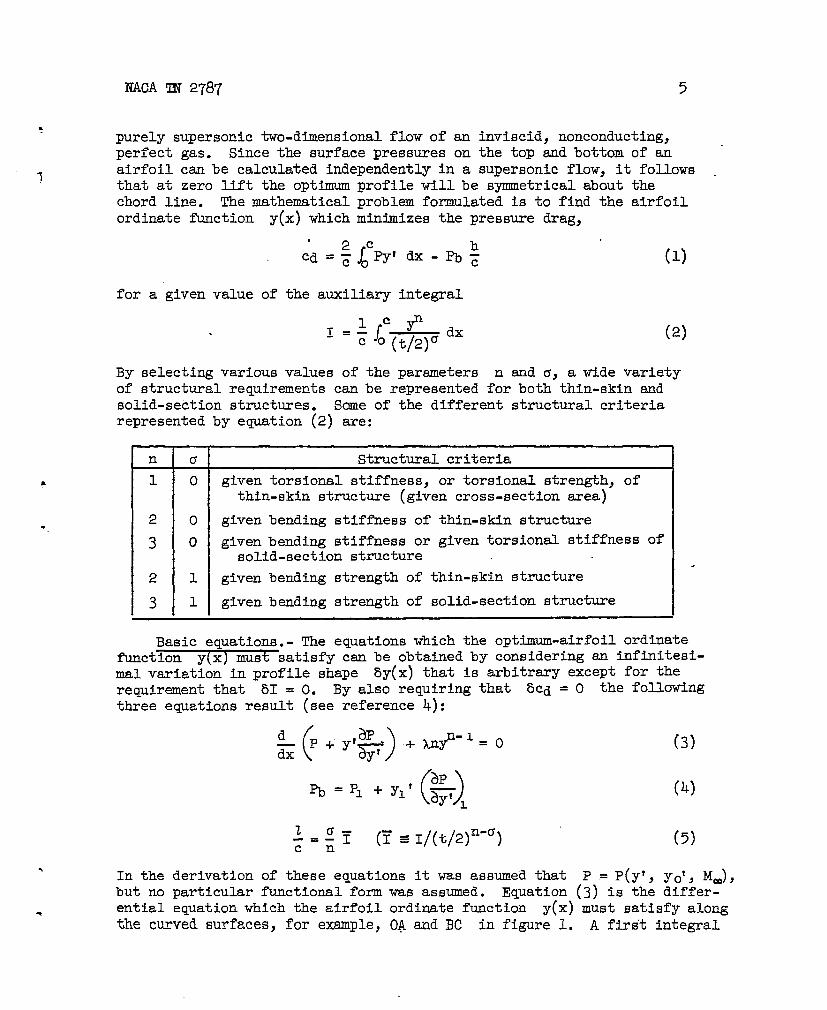
.purely supersonic two-dimensional flow of an inviscid, nonconducting,perfect gas. Since the surface pressures on the top and bottom of an ‘

? airfoil can be calculated independently in a supersonic flow> it fo~ows .that at zero lift the opttium profile will be symmetrical about thechord line. The mathematical problem formulated is to find the airfoilordinate function y(x) which rnintiizesthe

, 2Ccd=~ &m ‘dx -a

for a given value of the auxiliary integral

Ilc~dxs—‘F o (t/2)u

pressure drag,

hz (1)

(2)

By selecting various values of the parameters n and u, a wide varietyof structural requirements can be represented for both-thin-skin andsolid-section structures. Some of the different structural criteriarepresented by equation (2) are:

n 0 Structural criteria

1 0 given torsional stiffness, or torsional strength, ofthin-skin structure (given cross-section area)

2 0 given bending stiffness of thin-skin structure

3 0 given bending stiffness or given torsional stiffness ofsolid-section structure

2 1 given bending strength of thin-skin structure

3 1 given bending strength of solid-section structure

.

Basic equations.- The equations which the optimum-airfoil ordinatefunction y(xj must satisfy can be obtained by considering an infinitesi-mal variation in profile shape by(x) that is arbitrary except for therequirement that 51 = O. By also requiring that bcd = O the fo~o~uthree equations result (see reference 4):

2 :T-=.c

(~ = I/(t/2)n-a) (5)

.In the derivation of these equations it was assumed that P = P(y’, ye’, M=),but no particular functional form was assumed. Equation (3) is the differ-

* ential equation which the airfoil ordinate function y(x) must satisfy alongthe curved surfaces, for example, OA and BC in figure 1. A first integral

6 lUCA TN 2787

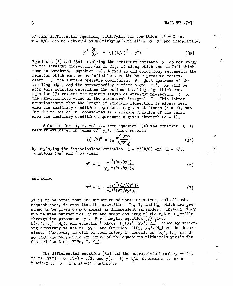
of this differential equation, satisfying the condition y’ = O at

Y= t/2, can be obtained by”multiplying both.sides by y’ and integrating.

2 aPY’ ~ = x [(t/2)n - yn] (3a)

Equations (3) and (Sa) involving the arbitrary constant x do not applyto the straight midsection (AB in fig. 1) along which the airfoil thick-ness is constant. Equation (4), termed an end condition, represents therelation which must be satisfied between the base pressure coeffi-cient m, the surface pressure coefficient PI Just upstrean of thetrailing edge, and the corresponding surface slope yl’. As will beseen this equation determines the optimum trailing-edge thickness.Equation (5) relates the optimum length of straight midsection 1 tothe dimensionless value of the structural integral ~. This latterequation”shows that the length of straight midsection is always zerowhen the auxiliary condition represents a given stiffness (a = O), butfor the values of n considered is a sizable fraction of the chordwhen the auxiliary condition represents a given strength (a = 1).

#

*

—

—

—

Solution for Y, H, and X.- ltrcmequation (Sa) the constant x isreadily evaluated in terms of yo~. There results

(jx(t/2)n = yof2 +

By employing the dimensionless variables Y =equations (Sa) and (3b) yield

F=l-yf2(aP/ayf)

Yo’2(W~Y’)o

A

(3b)

Y/(’t/Z) and H = h/t,A

(6)

and hence

(7)

It is to be noted”that the structure of these equations, and all sub-sequent ones, is such that the quantities Pb, I, tid Mm which are pre-sumed to be given do not appear as independent variables. Instead, theyare related parametrically to the shape and drag of the optimum profilethrough the parsmeter y’. For exsmple, equation (7) gives

) and equation 4 gives Pb(yli, ye’, M~, hence by select-H(Y1’S yOtj Mm >ing arbitrary values of ylt the function H(%, yet, Mm) cam be deter-mined. Moreover, as will be seen later, I depends on ye’, M@ and H,so that the parametric structure of the equa~ions ultimately yields thedesired function Il(Pb,I, Mm).

The differential equation (3a) and the appropriate boundary condi-tions. y(o),= O, y(s)=t/2, and y(s + Z) = t/2 determine x as afunction of y by a single quadrature. “-: —

.

r

NACA TN 2787

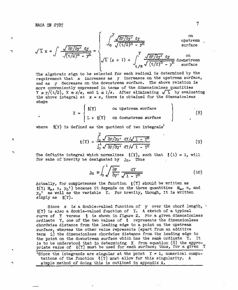
JTx=f

IJ- I(S +2)+y mm dYJ~,,J (t/2)n - f-’

7

onupstremn ,surface

ondownstream

surface

The algebraic sign to be sel~cted for each radical is determined by therequirement that x increases as y increases on the upstream surface,and as v decreases on the downstream surface. The above relation is.more conveniently expressed in terms of the dimensionless cwantitiesY ~ Y/(t/P), x =x/s,the above integral atshape

x=

/

and L ~1/s.x = s, there

3(Y) on

L+

where 5(Y) is defined as

Thefor

E(Y) on

After eliminating fi- by evaluatingis obtained for the

upstreem surface

downstream surface

the quotient of two integrals

dimensionlesss

(9)

definite integral which normalizes ~(Y), such that !%(1) = 1, willsake of brevity be designated by jn. Thus

If1 aP dY

Jn-o F J~(lo)

Actually, for completeness the function E(Y) should be written asE(Y; I&, n, Ye’) because it depends on the three quantities Mm, n, andYor as well as the variable Y. For brevity, though, it is writtensimply as E(Y).

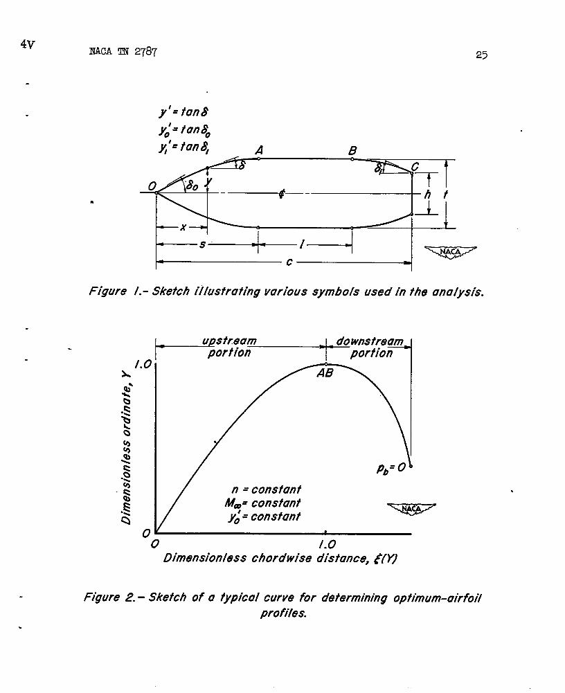
Since x is a double-valued function of y over the chord length, -5(Y) is also a double-valued function of Y. A sketch of a typicalcurve of Y versus g is shown in figure 2. For a given dimensionlessordinate Y, one of the two values of ~ represents the dimensionlesschordwise distance from the leading edge to a point on the upstreamsurface, whereas the other value represents (apart from an additiveterm L) the dimensionless chordwise distance from the leading edge tothe point on the downstream surface which has the same ordinate Y. Itis to be understood that in determining X from equation (8) the appro-priate value of g(Y) must be used for each surface; thus, for a given Y

%3ince the integrands are singular at the point Y = 1, numerical compu-tations of the function E(Y) must allow for this singularity. Asimple method of doing this is outlined in appendix A.

8 NACA TN 2787

the value of E(Y) appropriate to the downstream”surface always isgreater than for the upstream surface.

From the foregoing and the fact that E(Y) is independent of Pband u, it follows that a curve of Y versus ~(Y), such as is illus-trated in figure 2, determines the curved portions of an infinite numberof optimum profiles, all having the ssme valuresof YO1, &, and n. Itmay be noted that a (equation (5)) essentially determines the lengthof straight midsection which is to be placed between the two curvedportions after separating them at the point where ~ =fig. 2); whereas

1 (point A.B inPb (equations (4) smd (7)) essentially detetines H,

the value of Y beyond which the downstream portion of the curve ts notused in a given case. It is noted that although the chord is fixed,the value of ~ corresponding to the trailing edge is not. This isbecause ~ s x/s changes whenever s changes.

As maybe deduced from equation (7’),yl’ determines H for agiven n, ~,and YO1. Moreover, ylf determines ~ from equation (~).Hence, for any given value of base pressure the point on the downstreamsurface which corresponds to the trailing-edge position can be indicatedon each E(Y) curve. (See fig. 2 where the point corresponding to zerobase pressure is indicated.)

Solution for L,’~, t/c, and s/c.- Turning now to the determinationof the optimum length of straight midsection 1, one sees from equa-tion (~) that such a determination will also give ~. Since Z is afunction of yor and the given quantities n, a, n, and L, thisenables ye’,to be relatedif I is thethe following

— ..- . —,

—

—

—

A

the quantity used as a parsneter in the present analysis,to the quantity ~, which is a more convenient one to useactual quantity given. Starting with the definition of ~equations result:

—

~ = I/(t/2)n-a

. ;$ocbynd~ = ;f/s [1 - (1 - Yn)] m

[

Sc=- - -/oH(1 - Yn) + dYCB 1

or, by using the relation

dxl raP/3y’(11) .- –

==X 1-Y”:.

which follows from equations (8), (9), and (10), there results

2VITACATN 2787

. For convenienceas 7(H).

.

the right-hand member of this equation is defined

v(H) .~-]- d,

9

(12)

From equations (8) and (5),

~=L+~(H)

‘::~+~(H)

Combining this with the above relation between ~ and s/c gives

s n-a

c!- = n~(H) - cTq(H)

and

~ .(13)

(14)

●

RecaJling that H isM- n> Yo’)j one sees

. of IQ, n, u, ~, and

determined by ~ for a given _!i(Y)curve (giventhat equation (14) determines I as a function

Ye’= A convenient determination of ~, of course,can only be made if the function q(H) in addition to ~(Y) has beencomputed. The function 7(H), which for completeness sho~d be writtenas ?(H; Ma n, ye’), is somewhat easier to compute thsn E(Y) since itis not singular at Y = 1. Attention is called to the fact that all.theabove integrals with limits ranging from Y = O to Y = E, as in equa-tion (12), for example, really correspond to integration over bothcurved surfaces, first from Y = O to Y =1, andthenfromY=lto Y= H.

With the position ofmaximmun thickness determinedly equation (13),the maxhuun thickness ratio can be determined in terms of the surfaceslope at the leading edge.

(%)=?(s)Ot ()-=2:c (dY~i)o

or, from equation (n), in an alternate form

(15)

(15a)

Calculation of ureseure drag of an ODtimunlDrofile.- In reference 4it was shown that for linearized supersonic airfoil theory the pressure

10 IWCA TN 2787

drag coefficient of an optimum profile was a stiple algebraic functionof certain qusmkities such as H and S/C. Since these quantities areknown once the shape of the optimum profile is determined, a separateintegration is not required in order to calS_ulate.thepressure drag.Fortunately, a similar algebraic relation csn.also be developed for thepresent case. In so doing, integration.byparts is employed startingwith the defining equation for pressure drag.

(16).—

In these equations, and subsequent ones, the integration is carried out .only over the two curved portions since the straight midsection can con-tribute no drag. From equation (3a),

aPdJ?=—

()

~“ aP dx

a(l/y’) d y’= -Y’2 —

()by’ d ~

= -k [(t/2)n - #] d(~)

hence, substituting into equation (16) and again integrating by partsgives

:C=2d

The firsttion (4).

U;z [(t/2)n - (n + I)yn] dx

bracketed term on the right side v.snishesby vir~e of equa-The remaining integrals csm be simplified by noting that

There results.

()3Pcd =2Y:2 ~ [(n+ l-u)T -11o

(17)

This equation enables the pressure drag to be readily calculated if thebase pressure is given, since pb determines H for a given yoi andMm, and H determines ~ in accordance with equation (14). Thus,equation (17) involves the base drag tiplicitly, but not explicitly.For the special case of linearized supersonic flow,

aP—=by’

2/J~

and the above equation for cd can be shown to reduce to the correspond-ing equation for pressure drag developed in.reference 4.

*.—

.-

.———

.=

e-

—

r.

/J

*-

NJJCA‘IN

.

7When

2787

Closed-Form Solution for the Special Case of GivenCross-Section Area n = 1, a = O ●

the cross-section area of a profile is prescribed (n = 1,

11

a = O), corresponding to a given wing ~olume, torsional stiffiess,-ortorsional strength of a thin-skin structure, then the differentialequation (3) can be integrated immediately with respect to x to yielda solution in

The constantsandx=sto

Here P(0) is

closed form for the airfoil shape. There results

aP-lx= P+y~

F+ constant (18)

can be eliminated by evaluating this e~ressfon at x = Oobtain

;sx=g(y)=l- P+ yqap/ayq - P(0)

po + yo’(bpny’)o - ‘(O)

the pressure coefficient at y! . 0, and P. is the

(19)

pressure coefficient at x = O. For practical p@poses F(O) usuallycan be taken as zero, although strictly speaking it should be regarded

a as a small quantity compared to P. + yo’(8P/ay’)o. The parametricequations for Y and H in terms of yl sre the same as before, onlywith n = 1.

.

Theand

H=l- .y1f2(ap/ayqL

Yo’2(ap/ayt )0

(20)

(21)

general equation for the base pressure coefficient does not involve n,hence is the same as before.

(4)

The constant in equation (18) csn be evaluated at x = c insteadofatx=s. Combining such & evaluation with theyields the alternate e~-ression

x P + Yqaqayt) - m● -41-

C PO + Yo’(&/ay’)0 ‘pb.

which involves Pb instead of P(0). The equationscan be derived easily from the preceding equations.

. details, the following results are obtained:

above equation for ~

(22)

fOr t/C, S/C, and cdOnitting algebraic

12 NACA ~ 2787

BY evaluating equation (1.8)at x = c, and combining with equations (3b)

t 2yot2(aP/ay’)oc!‘=po + yo@/by?)o - pb

by evaluating equation (22) at x = s~ —

B1-

P(o) -PtJ-=c po + y~f(~p/ayt)O - ~

and by substituting n = 1 and a = O into equation (17),

Solution for the Specialn=~,

In reference 4 it was shown

Case of Givena = finite

1)

Thickness Ratio

that the limiting values n =oo,

(23)

(24)

(25)

a = finite, represent the auxiliary condition of a given airfoil thick-ness ratio. The mathematical simplification inherent in the use ofapproximate theories such as linearized flow enables the solution fora given thickness ratio to be obtained directly by passing the generalsolution to the limit as n-. For shock-expansion theory, though,a general-solution in closed explicit form cannot be obtained, andrecourse to the alternate method tndicated in reference 4 is required.This alternate method deals directly with the appropriate differentialequation, which, for the ‘caseof given airfoil thickness, becomes stiply

2 apY’ —=by’

constit (26)

which is satisfied by a profile composed of any number of straight seg-ments. As shown in reference 4, the constant in the above equation doesnot change over the entire chord, with the result that the upper halfof the profile forward of the ‘trailingedge is composed of-two straightlines, one extending from x = O = y to x = s, y = t/2, and the other

extending from x = s, y = t/2 .to the trailing edge x = c, y = h/2.The slope is discontinuous at the point where y = t/2. To obtain asolution using any given airfoil theory, it is necessary to satisfy thedifferential equation (26), the end condition (4), and the boundarycondition of a fixed thickness ratio.

Equation (17) for cd becomes indeterminate as n~m becaus~T*O. For this case, however, the shape is known and the pressure drag

.

-..—

n,

can be determined from simple

‘Cd)given t/c =

physical considerations:

~[Po -Fl(l -H) -~H] .

—

NACA ‘IN2787 . 13

.

.

APPLICATION OF

Flow at Infinite

ANALYSIS

Mach Nwnber

Prior to considering shock-expansion theory, the relatively simplecase of flow at infinite Mach number over slender airfoils with smallsurface curvature will be considered. For such conditions the pressurecoefficient on a surface facing upstream is proportional to the squareof the local surface slope, that is, P = Cy’2. Since the pressu~e coef-ficient is zero on any surface facing downstream it follows from physicalconsiderations that H = 1. Equation (4) is satisfied by requiring that

Y1’ = o- By consideration of the differential equation (Sa) as special-ized to the present case it follows that

f [011/6

$= J57=(2C)1’3 ~ y’ (1 - Ynp=

By substitution into equation (9), snd employment of gama functions toevaluate the intkgral in the denominator, there results

()2nr —++E(Y) = 3

001

(1 - Yn)-l’=dY.

r~r+(27)

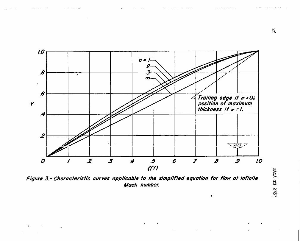
The function Yversus E(Y) is plotted in figure 3 for n = 1, 2, 3, and=.The infinite value of n corresponds to the auxiliary condition of agiven thickness ratio, and the optimum profile in this case is a wedge,

since()

+r : +1 and ~(Y)*Y as n+=. It is seen that there is

little difference between the three curves for finite n.

The other characteristic function needed for the complete determina-tion of an optimum profile is 7(H). ‘By substituting H = 1 in equa-tions (I-2),(13), (14), and (17), and employing equations (5), (10), and(28), the following expressions are obtained:

q(l) = +2n+3

s—=c!

T=

2-=c

(n - a)(2n + 3)

n(2n+ 3 - 20)

Q

ti+3-2c

3CT

n(2n + 3 - 2Cf)

(28)

(29)

(30)

(31)

.’

14XACA ~ 2787

..

(32)

If desired, this last equation for the pressure drag coefficient can bewritten in terms of 1 inetead of t/c, inasmuch as I is related tothe thickness ratio through equation (32). lt should be noted that theabove equations relate in closed form all pertinent properties of theoptimum profile to the given quantities 1, n, and a. Exmnples of opti-mum profiles determined with the aid of these equations are presentedsubsequently.

Shock-E~ansion Theory

When the oblique shock-wave and Prandtl-Meyer equations are combinedto calculate the pressure on an airfoil surface in supersonic flow, theresulting equations for P are quite involved. The appropriate equa-tion for ~PPyl, however, maybe obtained-by starting with the localdifferential relation

(35)

This point relation is formally the ssme as the corresponding relationapplied throughout sn entire flow field in linearized-supersonicairfoiltheory. The partial derivative bp/&5 is-taken tith Mmand 50 “heldconstant. Expressing equation (35) in terms of the pressure coefficientand free-stream conditions

there results

or, since

●

,

—

d

.

NACA TN 2787

.This equation appearscomputed readily with

15

fairly simple, but is not in a form which can bethe aid

as local pressure ratio p/pt-.

wave pt/Pt~ are tabulated.ting purposes is

aP 2 FM2

a

.

.

.

of existing tables where quantities suchand total-pressure ratio across a ‘shock

Thus, a more convenient form for calcula-

From this equation a numerical value of bp/bl can be determined fromtabulated oblique-shock and expansion characteristics once yet, M=,and the local slope y’ are specified.

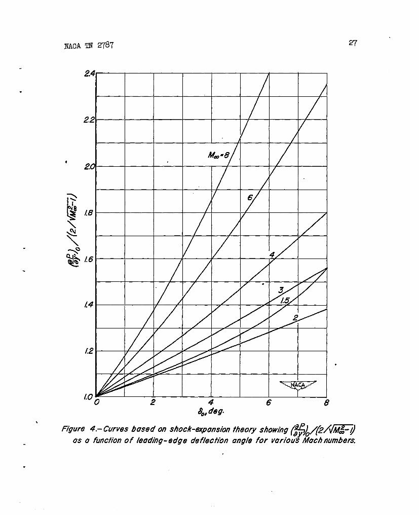
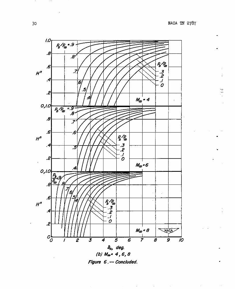
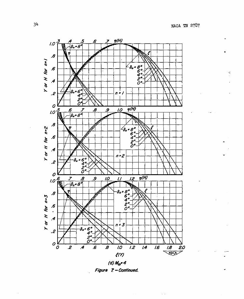
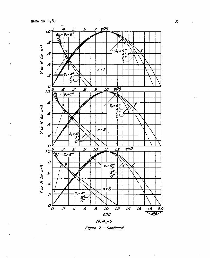
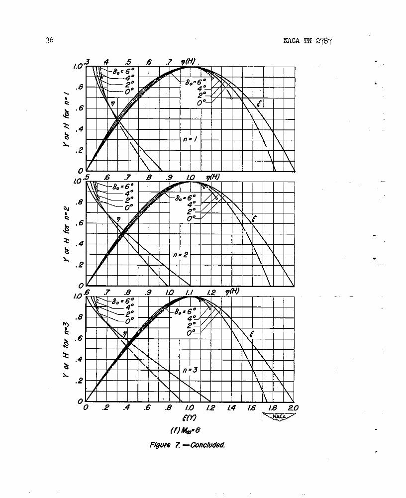
The functions E(Y) and 7(H) have been calculated for shock-, “expansion theory by substituting equation (36) into equations (9) and (12),respectively, and then performing the indicated integration graphicallyby the method outlined in appendix A. In this process other usefulquantities are calculated such as (~P/~y’)o and jn. The results arepresented in figures 4, 5, 6, and 7. In figure J+the quantity

(bP/ay’)o/(2/~), which is equal to (ap/bY’)o/[(a?/bY’).15 ~OJ

is plotted as a function of 80 for various values of Mm. StiiO~rly,

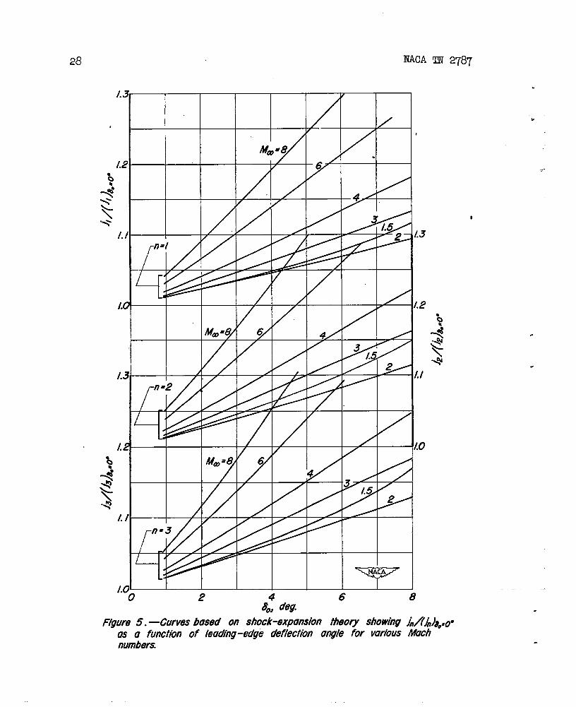
jn/(jn)boqo is plotted in figure 5. It is to be noted

where

kn =

Curves of F? versus 50

[

2forn=lIf/2for n = 2 1 (37)1.l+023...forn = 3

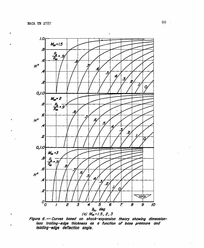
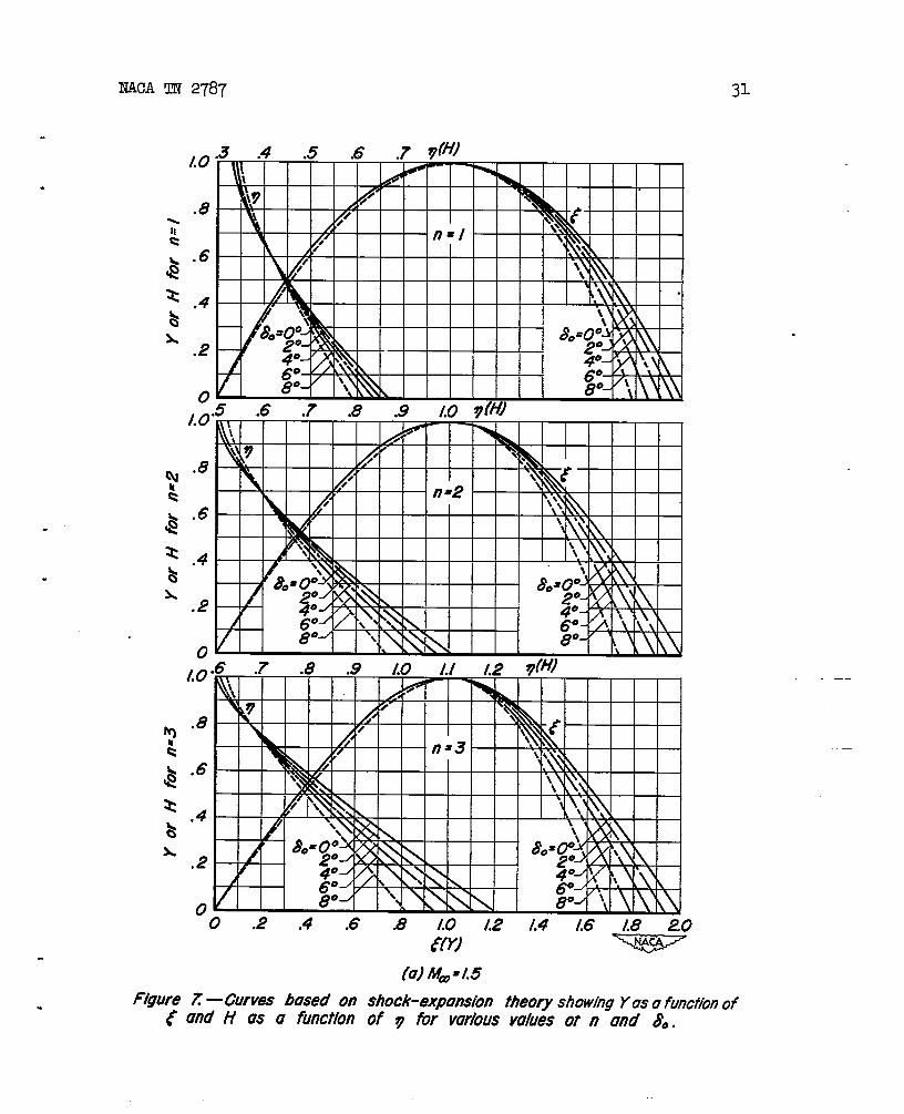
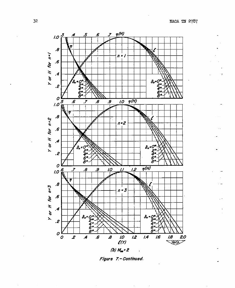
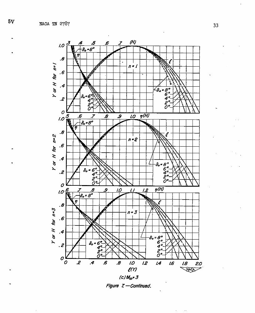
for various values of base pressure are pre-sented in figure 6, from which it is apparent that the dimensionlesstrailing-edge thiclmess increases if either the airfoil thicknessincreases (50 increases), or if the base pressure increases. In figure 7the functions E(Y) and v(H) for various 50,&, and n are presentedplotted in the form Y versus ~, and H versus q. The cties of Yversus E determine the shape of the optimum profile, while the curvesof E versus q are useful in determining I, S/C,curves of Y versus ~ have been terminated at thesmall circle) corresponding to zero base pressure.

EXAMPLES AND DISCUSSION

and t/c. Many of thepoint (indicated by

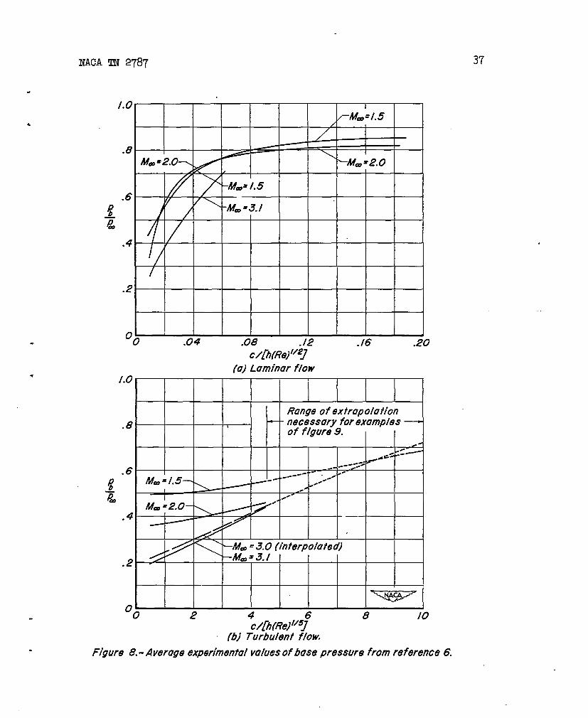
In order to determine an optimum profile it is necessary, of course,to know the base pressure. Experiments have shown that base pressure intwo-dtiensional flow depends principally on the Mach number, type of

,

16

boundary-layer(See reference

NACA TN 2787

flow, and the boundary-layer thiclmess at the base. . .

6.) Average experimental valu$s are shown in figure 8for both lsminar &d turbulent flow Ilotted .asa function of the parame-ters proportional to the ratio of boundary-layer thickness to trailing- ?-

edge thiclmess. Step-by-step details of the method of determining anoptimum profile by combining experimental base pressure data with thecurves of figures 4 to 7 me giyen in appendix B. ,

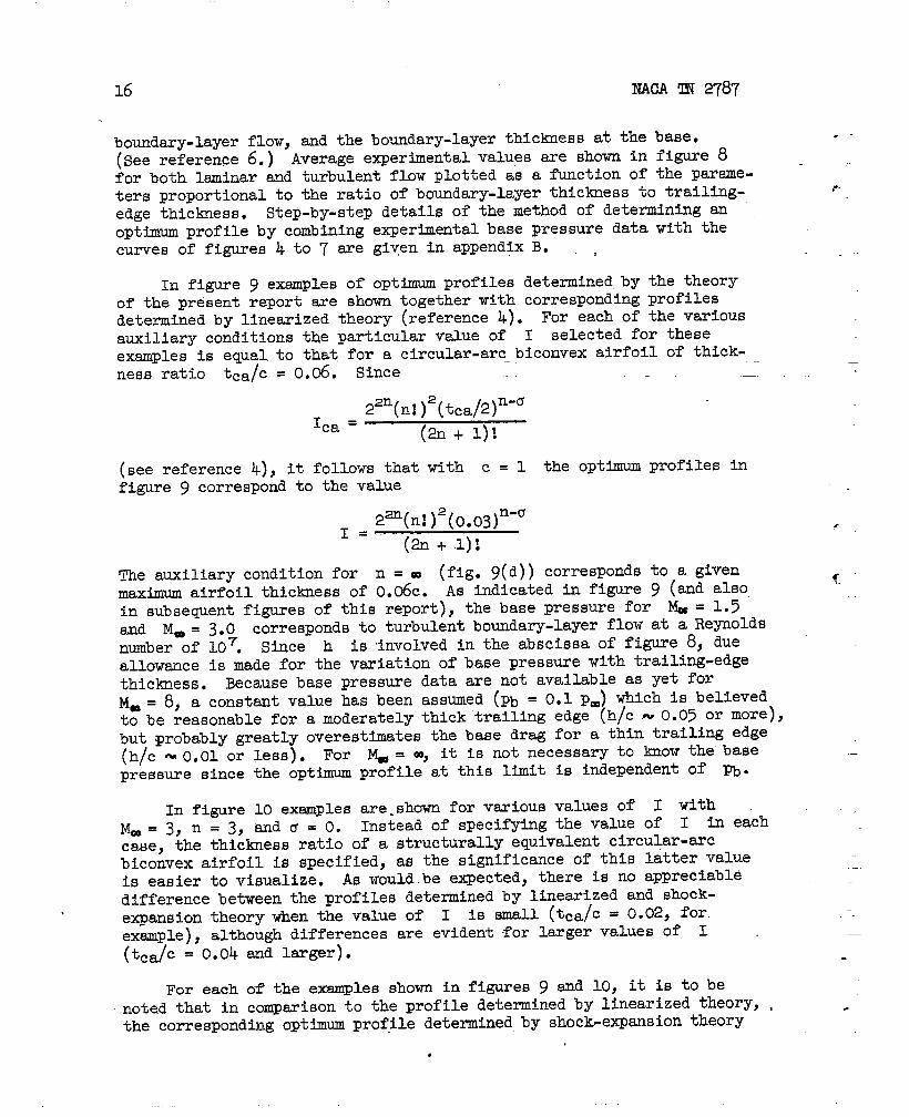
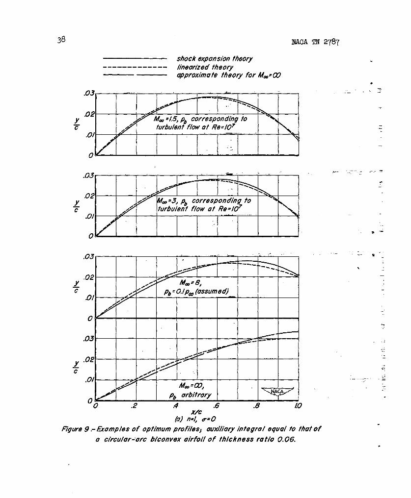
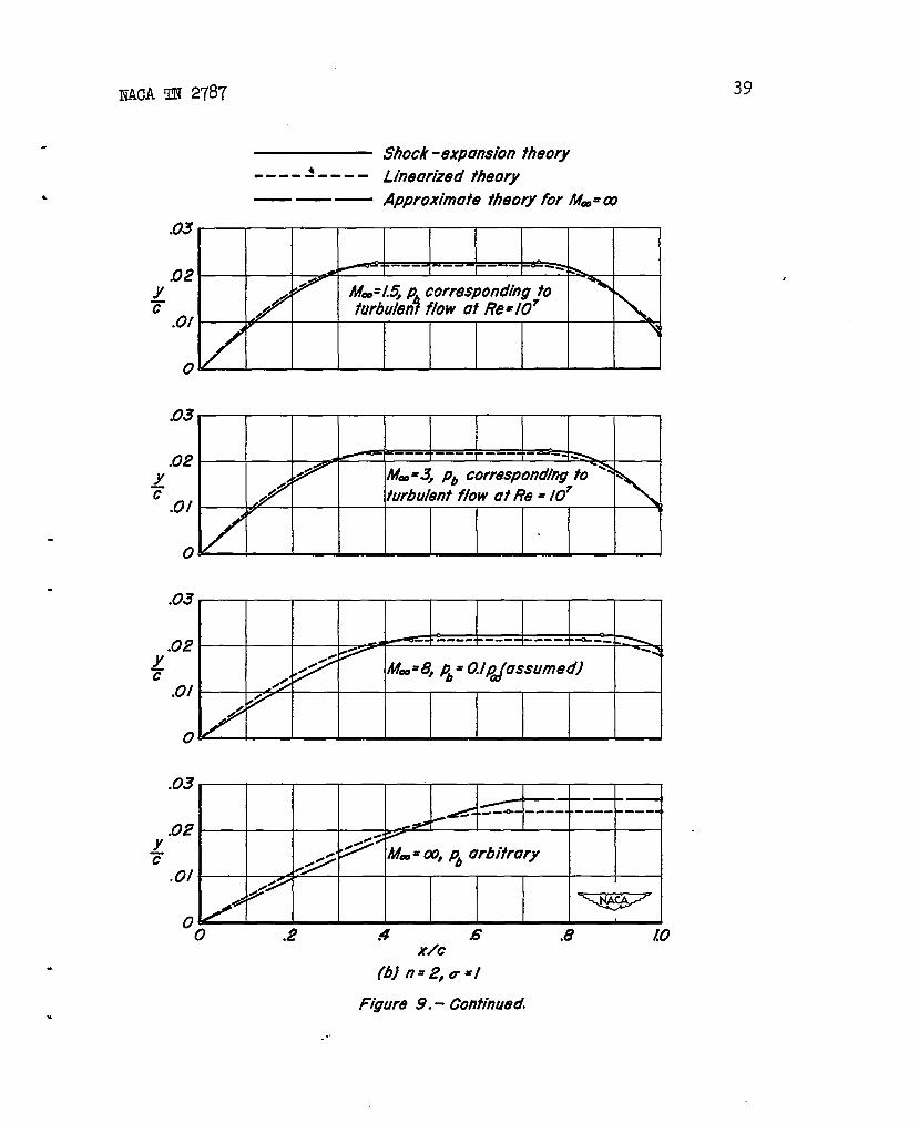
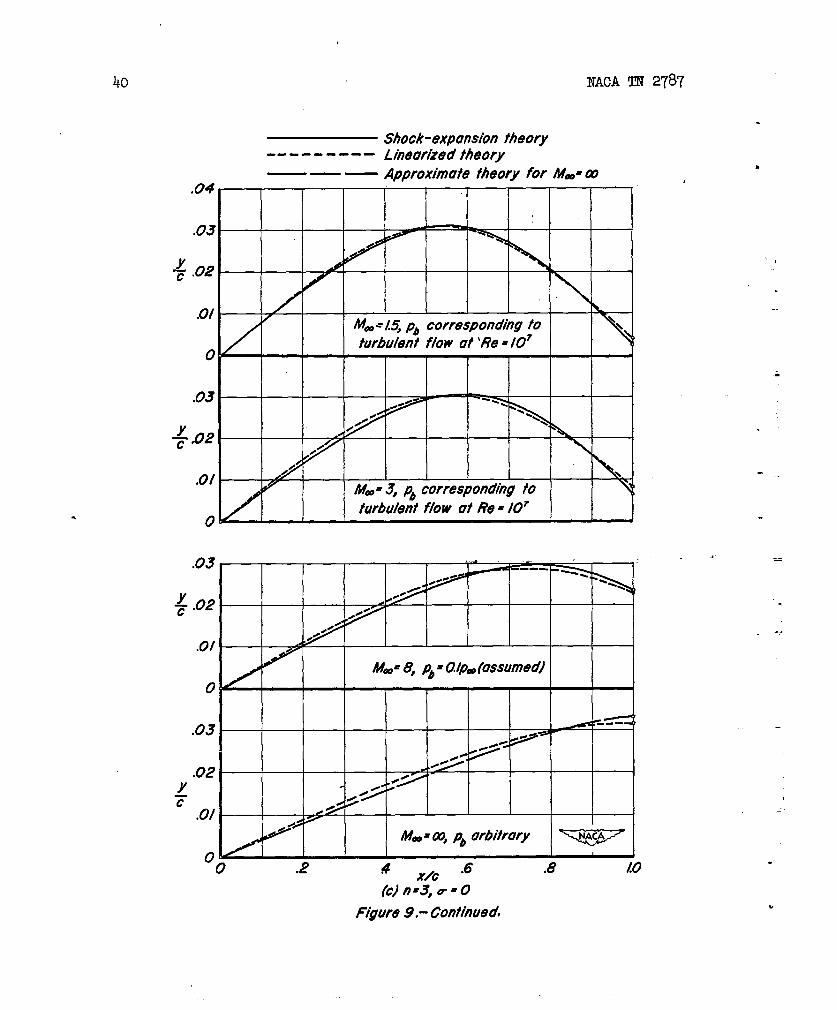
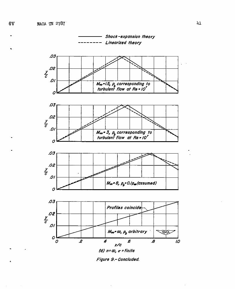
In figure 9 exsmples of optimum profiles determined by the theoryof the present report are shown together with corresponding profilesdetermined by linearized theory (reference 4). For each of the variousauxiliary conditions the Particular v~ue of I selected for ‘heseexamples is equal to that for a circular-arc biconvex airfoil of thick-ness ratio tea/C = 0.06. Since

.-

22n(n!)2(tca/2)n-a1ca = (2n + 1)!

(see reference 4), it follows that with c = 1 the optimum profiles infigure 9 correspond to the value

2m(n!)2(().()3)n-”I

*=.(2n + .1)!

The auxiliary condition for n = m (fig. 9(d)) corresponds to a givenmaxhnum airfoil thickness of 0.06c.

fAs indicated in figure 9 (and also

in subsequent figures of this report), the base pressure for & = 1.5and Mm= 3.0 corresponds to turbulent boundary-layer flow at a Reynoldsnumber of 107. Since h is involved in the abscissa of figure 8, dueallowance is made for the variation of base pressure with trailing-edgethickness. Because base pressure data are not available as yet forMm = 8, a constant value has been assumed (pb = 0.1 pa) which is believedto be reasonable for a moderately thick ’trailingedge (h/c N 0.05 or more),

.-

but Trobably greatly overestimates the base drag for a thin trailing edge(h/c * 0.01 or less). For B&= w, it is not necessary to how the base

pressure since the optimum profile at this limit is independent of pb.

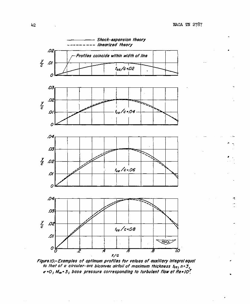
In figure 10 examples are.shown for various values of I withM==3,n =3, andu=0. Instead of specifying the value of I in eachcase, the thickness ratio of a structurally equivalent circular-arcbiconvex airfoil is specified, as”the significance of this latter valueis easier to visualize. AS would.be expected} there iS no appreciable

.-

difference between the profiles determined by linearized and shock-expansion theory when the value of I is small (tea/c = 0.02, for.exemple), although differences are evident for larger values of I

(t~a/C = O.O4 and.larger). .

For each of’the e-pies show in figures 9 -d 10s it is to benoted that in comparison to the profile determined by linearized theory, ,the corresponding optimum profile determined by shock-expansion theory

.

●

3V17~CA ZN 2787

.has a smaller slopeposition of maximum

over the portion of surface facing upstre~, athictiess farther aft, and a greater slope over the

* portion of surface facing downstream. This difference which increaseswith increasing Mach number is to be e~ected, as indicated in refer-ence 4, because the linearized theory overestimates the suction forcesand underesttites the positive pressure forces.

As regards drag coefficient, it is evident that drag calculationsb~sed on linearized theory cannot be used at hypersonic Mach numberssince the computed coefficient approaches zero as the Mach numberincreases. Also, it is to be remembered that linearized theory is con-siderably less accurate in predicting the drag of blunt-trailing-edgeairfoils than of sharp-trailing-edge airfoils, since the Busemann second-order terms for the Wstream and downstream surfaces do not cancel asthey do when the trailing edge is sharp.

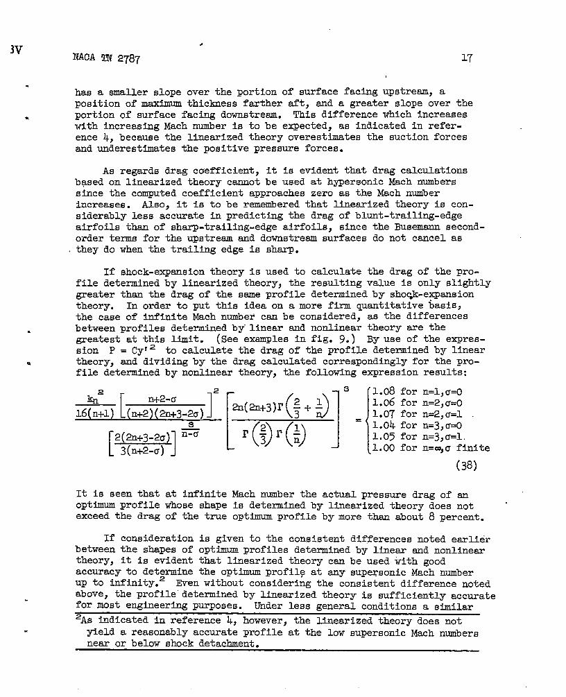
If shock-e~ension theory is used to calculate the drag of the pro-file determined by linearized theory, the resulting value is only slightlygreater than the drag of the ssme profile determined by she@-eWansiontheory. In order to put this idea on a more firm quantitative basis,the case of infinite Mach numbed can be considered, as the differences

. between profiles determined by”linear and nonlinear the~ry are thegreatest at this limit. (See exsmples in fig. 9.) By use of the expres-sion P = Cyf2 to calculate the drag of the profile determined by linear

e theory, and dividing by the drag calculated correspondingly for the pro-file determined by nonlinear theory, the following expression results:

2

422

[

n+2-a

16(ni-1) (n+2)(2n+3-2a)1[ 12@&2Q~

3(n+2-a)

It is seen thatoptimum profileexceed the drag

3

s

‘1.08 for n=l,c=O1.o6 for n=2,a=01.07 for n=2,cr=l1.04 for n=3,a=01.05 for n=3,cr=l,1.00 for n=~a finite

(38)

at infinite Mach number the actual pressure drag of anwhose shapeof the true

is determined by linearized theory ~oes not ‘optimum profile by more than about 8 percent.

If consideration is given to the consistent differences noted earlierbetween the shapes of optimum profiles determined by linear and nonlineartheory, it is evident that linearized theory can be used with goodaccuracy to determine the optimum profil~ at any supersonic Mach numberup to infinity.2 Even without considering the consistent difference notedabove, the profile”determined by linearized theory is sufficiently accuratefor most engineering purposes. Under less general conditions a similar

2As indicated in reference 4, however, the linearized theory does notyield a reasonably accurate profile at the low supersonic Mach numbersnear or below shock detachment.

NACA TN 2787

result also has been found in the recent investigation of Klunker andHarder (reference 7) which appeared while the present report was beingprepared. The shape of some of the optimum proPiles determined inreference 7, however, does not agree with the shape of analogous profilesin this report. For’example, it is indicated in reference 7 that theprofile of least drag for t/c = 0.06 has a--sharptrailing edge at allMach numbers below about 6, whereas the corresponding profiles shown infigure 9(d) indicate appreciable trailing-edge thickness even at Machnumbers of 1.5 and 3. This discrepancy is attributed to the arbitrarybase pressure curve assumed in reference 7 which does not correspond tomeasured data for thin trailing edge~. -

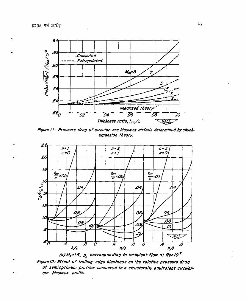
From an engineering viewpoint it is desirable to know how much lowerthe drag of an optimum profile is than that of a sharp-trailing-edgeprofile, and also how much the optimum profile can be altered withoutsignificantly increasing the drag. In order to-provide a basis of com-parison, the zero-lift pressure drag of a fsmily of sharp-trailing-edgecircular-arc biconvex airfoils of various thickness ratios has beencalculated by shock-expansion theory for the Mach number range between..1.5 and 8. The results are shown in figure 11. Thus, for any profilethe drag of a structurally equivalent (ssme value of I) circular-arcbiconvex profile can be determined readily from the curves in figure 11by simply calculating tca from the equation

I Ica == #n(n!)2(tca/2)n-o/(2n+ 1)!

Computations of drag have been made for a family of “semioptimum”profiles having arbitrarily selected values of trailing-edge bluntness H,a shape forward of the trailing edge that yields minimum foredrag for eachparticular H, and the ssme value of I “as “acircular-arc biconvex pro-file of thickness ratio tea. These calculations have been carried outfor tea/c = 0.02, 0.04, 0.06, 0.08, and 0.10 at Mach numbers of 1.5, 3,and 8, and for vtiious combinations of n and a. As in previousexamples, the base drag in each case was determined from the curves offigure 8 for turbulent-boundary-layerflow at Re = 107. The results areshown in figure 12 plotted in the form of a drag ratio versus H. Eachcurve corresponds-to a constant value of 1, and is identified by thethickness ratio (tea/c) of a circular-arc biconvex profile having thesane value for I. In order to maintain a constant value of 1, theactual thickness ratios (t/c)of the semioptimum profiles change somewhatas H varies between O and 1 (the ratio t/tea lies between about 0.90and 1.05 for the case n=l,u = O, between about 0.71 and 0.84 forn= 2, a = 1, and between about 0.97 and 1.08 for n = 3, cr= O). Foreach curve in figure 12 the semioptinmm profile having the minimum dragcoincides with the optimum profile determined from the curves of fig-ures 5 to 8. The ordinate of each minhaum point indicates the relativedrag of the opthnun compared to a structurally equivalent circular-arcbiconvex profile, while the rise on each side of the minimum indicatesthe ciragpenalty resulting from the use of too much or too littletrailing-edge thickness. It may be noted that some of the curves do not

●

..

-——..

—-.

..——

—.-

——

“

.

NACA TN 2787 19

. cover the complete range of values of H. In all such cases, however,sufficient calculations were made so that the minimum point was bracketed.

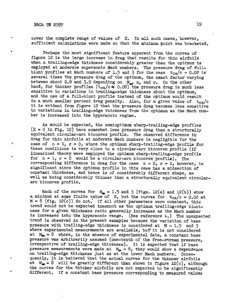
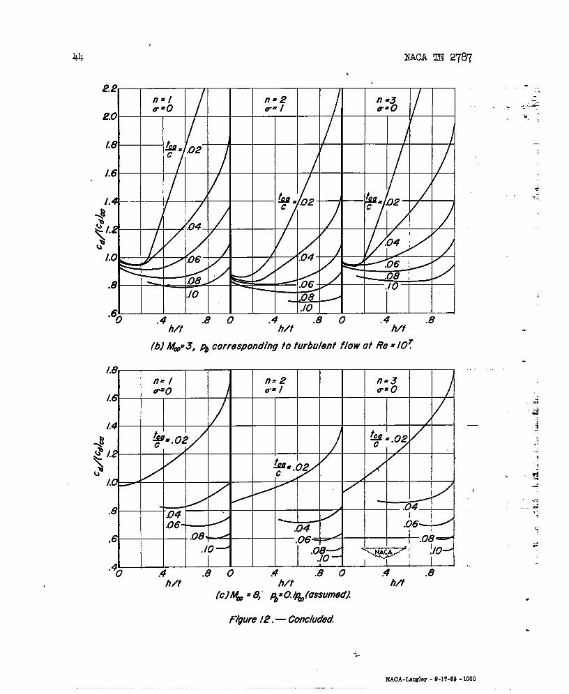
. Perhaps the most significant feature apparent from the curves offigure 12 is the large increase in drag that results for thin airfoilswhen a trailing-edge thickness considerably greater than the optimum isemployed at moderate supersonic Mach numbers. The pressure drag of full-blunt profiles at Mach numbers of 1.5 snd 3 for the case tc$c = 0.02 isseveral times the pressure drag of the optimum, the exact factor varyingbetween about 2.8 and 3.9 depending on Mti n, and a. On the otherhand, for thicker profiles (tea/c~ 0.08) the pressure drag is much lesssensitive to variations in trailing-edge thickness about the optimum,and the use of a full-blunt profile instead of the opthnun would resultin a much smaller percent drag penalty. Also, for a given value of tea/Cit is evident from figure 12 that the pressure drag becomes less sensitiveto variations in trai~ng-edge thickness from the optimum as the Mach num-ber is increased into the hypersonic regime.

As would be ~ected, the semiopttium sharp-trailing-edge profiles(H = O in fig. 12) have somewhat less pressure drag than a structurallyequivalent circular-src biconvex profile. The observed difference indrag for thin airfoils at moderate Mach numbers is negligible for the

* case of n = 1, cr= O, since the optimum sharp-trailing-edge profile forthese conditions is very close to a circular-arc biconvex profile (iflinearized theory were employed the optimum sharp-trailing-edge profile

. for n=l,u = O would be a circular-arc biconvex profile). Thecorresponding difference in drag for the case n=2,cr = 1, however, issignificant since the optimum profile in this case has a midsection ofconstant thickness, and hence is of considerably different shape, aswell as being considerably thinner than aarc biconvex profile.

Each of the curves for ~ = 1.5 anda minimum at some finite value of H. but

structurally equival&k circular-

3 (figs. 12(a) and 12(b)) showthe curves for tea/c = 0.02 at

M =8 (fig. 12(c)) do not; If all o~her parameters were constant, thistrend would not be expected inasmuch as the optimum trailing-edge-blunt-ness for a given thickness ratio generally increases as the Mach numberis increased into the hypersonic range. (See reference 4.) The unexpectedtrend is observed in the present exsmples because the variation of basepressure with trailing-edge thickness is considered at M = 1.5 and 3where expertiental measurements sre available, butiit is not consideredat & = 8 where, in the absence of expertiental data, a constant basepressure was arbitrarily assumed (one-tenth of the free-stream pressure,irrespective of trailing-edge thiclmess). It is expected that if basepressuremeasurements were made at IQ= 8, they would show a dependenceon trailing-edge thiclmess just as at the lower Mach numbers. Conse-quently, it is believed that the acttil curves for the thinner airfoilsat Mm = 8 will be greatly different than shown in figure 12(c), althoughthe curves for the thicker airfoils are not e~ected to be significantlydifferent. If a constant base pressure corresponding to measured values

20

on thick trailingfor tc~c = 0.02than at u = 8.

NACA TN 2787

edges were assumed at & = 1.5 and 3, the curves .

would rise starting from H = O even’more steeplyThis illustrates the necessity of considering the

dependence–of base pressure on trailing-edge thickness in such an .=

analysis.s

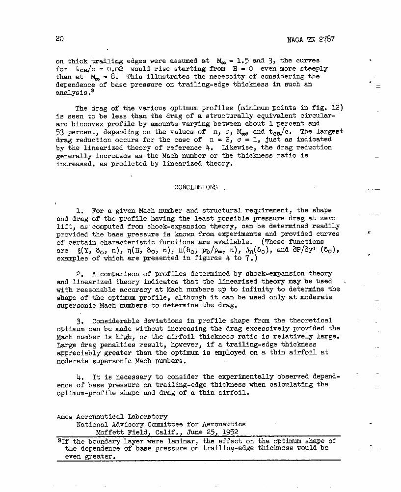
The drag of the various optimum profiles (mintium points in fig. H)is seen to be less than the drag of a structurally equivalent circular-arc biconvex profile by amounts varying between about 1 percent and53 percent, depending on the values of n, a, Ma and tca C./ The largestdrag reduction occurs for the case of n = 2, CT= 1, just as indicatedby the linearized theory of reference 4. Likewise, the drag reductiongenerally increases as the Mach number or the thickness ratio isincreased, as predicted by linearized theory.

CONCLUSIONS .

1. For a given Mach number and structural requirement, the shapeand drag of the profile having the least possible pressure drag at zerolift, ascomputed from shock-expansion theory, can be determined readilyprovided the base pressure is known from experhnents and provided curves x

of certain characteristic functions are available. (These functionsare E(Y, 5., n), q(H, Go, n), H(50, Pb/P~, n), jn(~o), and bphY’ (bo)~ ~exsmples of which are presented in figures 4 to 7.)

2. A cmparison of profiles determined by shock-e~ansion theoryand linearized theory indicates that the linearized theory may be Used twith reasonable accuracy at Mach numbers up to infinity to determine theshape of the optimum profiles although it cw be used only at moderatesupersonic Mach numbers to determine the drag.

—

3. Considerable deviations in profile shape frcm the theoreticaloptimum can be made without increasing the drag excessively provided theMach number is high, or the airfoil thickness ratio is relatively large.Large drag penalties result, hpwever, if a trailing-edge thicknessappreciably greater than the optimum is employed on a thin airfoil atmoderate supersonic Mach numbers.

4. It is necessary to consider the expertientally observed depend- - -ence of base pressure on trailing-edge thickness when calculating theoptimum-profile shape and drag of a thin airfoil.

—

Ames Aeronautical LaboratoryNational Advisory Co?mnitteefor Aeronautics .

Moffett Field, Calif., June 2’j, 195231f the bo~darY layer were l~inarj the effect on the optimum shape of

the dependence of base pressure on trailing-edge thiclmess would bew-

.

.

NACA ‘IS’T2787 21

APPENDIX A

MBTHOD OF cALCULATING 5(Y)

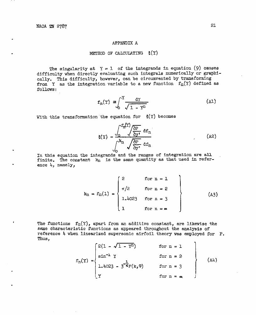
The singularity at Y = 1 of the integrands in equation (9) causesdifficulty when directly evaluating such integrals numerically or graphi-cally. This difficulty, however, canbe circumvented by transformingfrom Y as the integration variable to a new function fn(Y) defined as

follows:

[

Yfn(Y) =

&

(Al)

Yn

With this transformation the equation for ~(Y) becomes

.

In thisfinite.

. ence k,

,(Y) ]’n(y~dfn‘ % aPdfn

(A2),

Jr by’

equation the ‘integrandsand the ranges of integration ~e auThe constant kn is the ssme quantity as that used in refer-nsmely,

112 forn=l

m/2 forn=2kn =fn(l) =

1.k023 forn=3

1 f’orn=rn

(A3)

R The functions fn(Y), apart from an additive constsnt, sre likewise thessme characteristic functions as appeared throughout the ~alysis ofreference h when linearized supersonic airfoil theory was employed for P.Thus,

1

2(1 - J-) forn=l

sin-~ Y forn=2f~(Y) =

1

(Ak)

1.4023 - 3~F(k, 9) for n = 3

.Y forn=rn. j

22

where F(k,~) is the incomplete elliptic integralmod!ulus k = sin 75° = 0.9659, ~d ~plitude

$). ~o~-. (J-? -1 +--Y)

(J’3+ 1-Y)

NACA TN 2787

of the first kind of ?...

.

With the transformation to fn} the integrals in equation (A2) areevaluated by first selecting a number of values of yf ranging from yofto large negative values. For each y’ the ordinate Y is computedfrom equation (6), fn from equation (Ak), ~d ?lP/~y~ from the particu-lar airfoil theory. A plot is then maae of ~Pfiy’ versus fn in orderto evaluate the integrals determining E.(Y).

NACA ‘IN2787 . 23

.APPENDIX B

. DETAILS OF METHOD OF DETERMINING THE SHAPE AND DRAG OF

AN OPTIMUM PROFILE BY SHOCK-EXPANSION METHOD

In the shock-expansion equations the leading-edge deflectionangle b. is a more convenient parameter to use them the given valueof I, hence the steps outlined below involve an iterative procedure.

(1) Assume values of 80 and pb/p=

(2) Read value of Hn from figure 6 ~d ccmpute H

(3) Read values of E(H) and v(H) from figure 7; compute ~ fromequation (14) and s/c from equation (13)

(4) Read value of (aP/ay’)0 from figure 4, jn/(jn)~o s Oo

from figure 5; compute (jn)bo . ~o from equation (37),

t/c from equation (15a).

(5) Compute I = ~ (t/2)n-u

. By comparison of the computed value of I with the given value, a newvalue of 50 can be estimated. Also, frcm the computed value of h/c,the experimental base pressure curves in figure 8 yield a new value of

Pb/Pa●By repetition of the above steps until the final computed value

of I is equal to the given value, and the final computed value of h/ccorresponds to the final base pressure assumed, all characteristics”(~0, t/c, S/C, H, 6(Y), (aP/ay’)0, Jnj and ~) of the optimum profile aredetermined. The pressure drag is then calculated from equation (17).

24 JYACATN 2787

REFERENCES s-

1. Saenger, Eugen: Raketen-Flugtechnik. R. Oldenbourg, Munchen und xBerlin, 1933.

2. Ivey, H. Reese:/

Notes on the Theoretical Characteristics of Two-Dimensional Supersonic Airfoils. NACA TN 1179, 1947.

3. Smelt, R.: Problems of Missiles at Extreme Speeds. NOLR 1131, -Symposium on Ordnance Aeroballistics, June 1949, PP. 51-68.

A-

4. Chawan, Dean R.: Airfoil Profiles for llinhnumPressure Drag atSupersonic Velocities -.General Analysis and Application to

.—

Linearized Supersonic Flow. NACA TN2264, 1951..

5. Eggers, A. J., Jr., and Syvertson, Clarence A.: Inviscid Flow AboutAirfoils at High Supersonic Speeds. NACA TN 2646, 1952.

6. Chapman, DeanR., Wtibrow, William R., and Kester, Robert H.:Experimental Investigation of Base Pr-essureon Blunt-Trailing-Edge J

—

Wings at Supersonic Velocities. NACA TN 2611, 1952...=

7. Klunker, E. B.,and Harder, Keith C.: Comparison of Supersonic.

Minimum-Drag Airfoils Determined by Linear and Nonlinear Theory.NACA TN 2623, 1952. .

4V

.

.

m

mm TN 2787

.

.

Figure !.- Sketch illusfruting various symbols used in the anuiysis.

-z:; I downsfre~Dorfion.

/.0’ I .

L

JLj’b

“sk*~.3Qc n = constant

.$Q

o 90 /.0

Dimensionless choro’wise o’istunce, [(V

Figure 2.- Sketch of o typical curve for

profiles.

determining optimum-airfoil

Lo

.8

.6

Y

.4 -

.2

mm

/)s/.

2-

,a–

~ - Wiling 8tfgt? if e = o;position of muximum

thickness if w =1.

o f .2 .3 # .5 .6 .7 .8 .9 Lo

#Y)

Figure 3- Characteristic curves applicable to the simplified equation for flow at Infinite g

~ach numbef El

2* %

‘

, ,

.

.

.

NACA ZN 2@7 27 “

2.4

2.2

/.0

/$f&.8

/

● /

/ A

/

//

/ /

,

/ I

) 2 4 6 8& deg.

●

Rgure 4.-Curves bused on shock-mponsion theory showing ~~~/@/~MX~

os o function of Ieudiig - edge deflection angle for variou3’ Mach numbers.

28

.

4/

/

/ / /#●

/ //

/4

0 28.; deg.

Z-4

+

3/.5 2-

wFigure 5. —Curves hosed on shock-expansion theory showing ~/(jJ8a=00

as a function of leading-edge deflection angle for wrlous Mdch -numbers

.

“

.

—. —

.

.

NACA m 2787 29

.

.

.

.

H“.4

.2 t / / / /

(2,/.0 ‘I I I I /

M@=3

“0/23456 789108., deg

(0” A&= /.5, 2,3

Figure 6.— Curves bused on shock-expansion theo~ showing dimension-less trailing-edge thickness us o function of hose pressure mdleading-edge deflection ongte.

30 NACA TN 2787

/+n

o,

/in

8., deg.

(b) M-” 4,6,8

—--

.

if

.

.Figure 6. — Concluded.

NACA TN 2787 31

.

●

.

/.0

0/.0

0

,.3 .4 .5 .6 .7 @)

.

Lo

h “8&~ .6

x .4b

L .2

00 .2 .4 .6 - - -

Figure Z —Curves hosed on{ and H us u function

.8 /.2 /.4 /.6 /.8 2.0j%) w

(a) Mm=l.5

shock-expansion theory showing Y os o function ofof T for various values or n and &.

32 NACA TN 2787

“

/.0

0/.0

0

.5 .6 .7 .8 .9 10 7(W

O 2 .4 .6 .8 LO 12 /.4 16 L8 2.0

W)

.

.

—

.

—

.—

@)MD’2 .

Figure Z-Continued.

5V NACA TN 2787 33

.

.

.

.

0

A

(c)M&= 3

Figure Z —Gonthued.

34 NACA TN 2787’

/.0

n

.3 .4 .5 .6 .7 v(W

T

I .2 .4 .6 .8 1.0 1.2 1.4 /.6 k8 2.0

t[v w

.

—

(d) M@=4

Figure Z- Oonfinuea. ●

NACA. TN 2787—

35

/ ‘

.:.5 .6 .7 .8 .9 Lo M)f.u

/.0”’

.8~

: .6e

x .4a

L .2

0-0 .2 .4 .6 .8 /.0 /.2 L4 16 /,8 2.0

[(H) v

[e) M&6

Figure Z — Continued

36 NACA TN 2787

/.0”3 4 “5 “6 .7 VW.

.8

.6

.4

.2

0

/ I I I I I \ l\ I

.8

.6

.4

.2

n‘.6 .7 .8 .9

/.0 10 /./ 12 v~~’

.8

.6

.4

.2

00 .2 .4 .6 .8 1.0 L2 14 L6 /.8 2.0

.

.—

+

.

-. —

[(v -(f)&=8

Figure Z —Concluded

.

/.0

.8

.

.4

.2

0

I I I I t I J’+f==m I

) .04 .08 ./2 .16 .20c/[h(Re)”2]

(0)Lamini7r flow1.0

Range of extrapolation

.8- - necessary for examples —\

of figure 9...”

/ . ~---.-s. -

.6- ..--.0

> ----- ----- #O.-~“

~ I~ /@-

M’ =2.0– < / p#“

.4- ~

-M* =3.o (’inferpoluted)e

.2 / —M* =3. /

v

00 2 4 8 10c/[h(Re)1J5]6

(b) Turbulent flow.

Figure 8.- Averoge experimental values of base prt?ssure from reference 6.

shock exponsion theory------------- Iineorized theory

upproximofe theory for A&= W

.03

.02

turbulent flow of Re=107.0/

o

.03.-. , -. .. . ..

( I.02 1

ky I&=3, P. corresponding to ] ‘% I

o

.01

0o .2 .4 .6 .8 /!0

x/c(o) n=~ fl=O

Figure 9.- EYomples of optimum pro filesj ouxiliury integrol equol to thot of

L--

—

●

✎✎ �✚�

—

.- ...- ,...=

..

..:---.—

.s.——

..,.

0 circulur-orc biconvex oirfoil of thickness rotio 0.06.

.

.

Shock-expansion theory

---- 2---- Linearized theory—— — Approximate theory for AL= w

.03

.02----- ---- ---- P- -=d ~ t

Y Mm=@ p correspondthg toF turbulen+ flow d Re=107

.0/

o

.03

.02YF

.0/

o

.03, 4

.--e - ----- ----- ----- ~-H

.02 eY /“

/ ~Mm=m, ~ arbitrary

F

.0/

ORo .2 .4 E .8 [0

x/c

(b)n=2, e=l

Figure 9.- Continued

,..

NACA TN 2787

.

Shock-expansion theory--------- Lrheartied theory—. . Approximate theory for A&= w

.04. .

.03

.02 A

0/

o

.03

+ X22

.0/

turbulent flow at Re = /07 Io

.03

+ .02

.0/

.03

.02

n“o .2 # x/c .6 .8 Lo

.,

.

b

‘,

.

—

(c) ns3, u= oFigure 9.- Gontinuede

w

41

.

. .

d

Shock -expansion theory

-------- Linearized theory

.03

.02YF

.0/

o

.03

/.02

Y +●

7.0/

o

.03

.02

oM..= 8, pb=O.lpJ..ssumed)

.03

.02YF

.0/ / -

00 .2 f? .8 .8 10

x/c

(d) n= m, u= finite

Figure 9.- Concluded

NACA TN 2787

Shock- exponsion theory--------- linearized theory

.02Profiles coincide wifhh width of line

.0/

o

.03

.02

.0/

o

.04

a

.02/ ‘

“\ \ten/C =.06

.0/

o

x/c

F@we 10.-Examples of optimum profiles for volues of auxiliary integrol equolto that of o circuhr- me biconvex oirfoi/ of maximum thickness tea; n= 3,

~ =0; Mm= 3, hose pressure corresponding to turbulent flow at Re =/0?

.

—

9.

2787.

.64-,/’/

.6 ‘0

2 —Con@ed /

------ Extrapolated/“’ /’,/ 0

.60 4

&+8

.58 /

.56 “ /

54 t1linearized theory’ ‘

520 .02 .04 .06 .08 Jo

43

Thich9ss rotio, tCo/c--

Rgurell.-Pressure drug ofclrculor-arc bicmvmolrfoils o’eterminedbysbock-mpansion theory.

2.2~.f nn2 nm3~.o @.*/ @..o

20

L8 It~~ ftca tca

7.02L6

-z .04 .04$14

/ /

12// ‘

/f

/ ,

.Oy/

.Oy * ~10 ~! / ) /

.08 / ‘do

“ yI

— v“.60 .4 .8 0 .4 .8 0 .4 . .8

h/~ h/~

(a) M’ =1.5, pb corresponding to

Figure 12.- Effect of trailing-edge bluntness

of semioptimum profiles compared to aarc bicorwex profile.

h~

turbulent flow utRe=107

on the relutlve pressure dregstructurally equivulen t circuk7r-

44 NACA m 2787

L

2.2~.~

2.0C=o

1.8 1

c

/.6

4 / i

8/”c

‘we /.\2

/ ~/

Qe}

/

\ ~ .08.8 — d

~ .10.10 .08

.60./0

.4 .8 0 .4 .8 0 .4 .8h/t h/t Wt

-.

. .—..-..___—

.

(b) M’=3, pb corresponding to turbulent flow at Re = 10?

.Z.:

.1

.

Fl@re 12. — Concludedb

-..

NACA-Lnngley-9-17-62-1000