Embed Size (px)
Citation preview

https://ntrs.nasa.gov/search.jsp?R=19920015081 2020-01-26T21:14:32+00:00Z

H
m
I
T _

NASA Conference Publication 3145
TwentiethNASTRAN o
Users'Colloquium
Computer Software Management and Information CenterUniversity of Georgia
Athens, Georgia
Proceedings of a colloquium held in
Colorado Springs, Colorado
April 27-May 1, 1992
National Aeronautics and
Space Administration
Office of Management
Scientific and TechnicalInformation Program
1992


FOREWORD
NASTRAN® (NASA STRUCTURAL ANALYSIS) is a large, comprehensive,nonproprietary, general purpose finite element computer code for structuralanalysis which was developed under NASA sponsorship and became available tothe public in late 1970. It can be obtained through COSMIC® (ComputerSoftware Management and Information Center), Athens, Georgia, and is widelyused by NASA, other government agencies, and industry.
NASA currently provides continuing maintenance of NASTRAN through COSMIC.Because of the widespread interest in NASTRAN, and finite element methods ingeneral, the Twentieth NASTRAN Users' Colloquium was organized and held at theSheraton Colorado Springs, Colorado Springs, Colorado on April 27 - May I,1992. (Papers from previous colloquia held in 1971, 1972, 1973, 1975, 1976,1977, 1978, 1979, 1980, 1982, 1983, 1984, 1985, 1986, 1987, 1988, 1989, 1990and 1991 are published in NASA Technical Memorandums X-2378, X-2637, X-2893,X-3278, X-3428, and NASA Conference Publications 2018, 2062, 2131, 2151, 2249,2284, 2328, 2373, 2419, 2481, 2505, 3029, 3069 and 3111.) The TwentiethColloquium provides some comprehensive general papers on the application offinite element methods in engineering, comparisons with other approaches,unique applications, pre- and post-processing or auxiliary programs, and newmethods of analysis with NASTRAN.
Individuals actively engaged in the use of finite elements or NASTRANwere invited to prepare papers for presentation at the Colloquium. Thesepapers are included in this volume. No editorial review was provided by NASAor COSMIC; however, detailed instructions were provided each author to achievereasonably consistent paper format and content. The opinions and datapresented are the sole responsibility of the authors and their respectiveorganizations.
NASTRAN_ and COSMIC® are registered trademarks of the National Aeronautics andSpace Administration.
i i i PR'ECEDiNG PAGE BLANK NOT FILMED


CONTENTS
FOREWORD ...............................
le NASTRAN INTERNAL IMPROVEMENTS FOR 92 RELEASE
by Gordon C. Chan
(UNISYS Corporation)
Q EVOLUTION OF A NASTRAN TRAINER .................
by H. R. Grooms, P. J. Hinz and M. A. Collier(Rockwell International)
. ANIMATION OF FINITE ELEMENT MODELS AND RESULTS .........
by Robert R. Lipman
(David Taylor Research Center)
, ACCURACY OF THE TRIA3 THICK SHELL ELEMENT ............
by William R. Case, Marco Concha and Mark McGinnis
(NASA/Goddard Space Flight Center)
¢ VALIDATION OF THE CQUAD4 ELEMENT FOR VIBRATION AND SHOCK ANALYSISOF THIN LAMINATED COMPOSITE PLATE STRUCTURE ...........
by Douglas E. Lesar(Naval Surface Warfare Center)
6o A CASE OF POOR SUBSTRUCTURE DIAGNOSTICS .............
by Thomas G. Butler
(Butler Analyses)
e ALTERNATIVE METHODS TO MODEL FRICTIONAL CONTACT SURFACES USING
NASTRAN .............................
by Joseph Hoang(GE Government Services)
8. HIERARCHICAL TAPERED BAR ELEMENTS UNDERGOING AXIAL DEFORMATION
by N. Ganesan and S. K. Thampi(GE Government Services)
go TRANSIENT THERMAL STRESS RECOVERY FOR STRUCTURAL MODELS .....
by William Walls
(McDonnell Douglas Space Systems Co.)
10. TRANSIENT LOADS ANALYSIS FOR SPACE FLIGHT APPLICATIONS .....
by K. Thampi, N. S. Vidyasagar and N. GanesanS'(GE Government Services)
11. ACOUSTIC INTENSITY CALCULATIONS FOR AXISYMMETRICALLY MODELED
FLUID REGIONS .........................
by Stephen A. Hambric and Gordon C. Everstine(David Taylor Research Center)
Page
iii
1
9
23
26
51
I00
116
124
134
154
166
v pR_CE'I)!r,_ PAC,E IBLAN_ _T FILMED


N92-24325
NASTRAN INTERNAL IMPROVEMENTS FOR 92 RELEASE
by
Gordon C. Chan
NASTRAN Maintenance Group
UNISYS Corporation
HuntsviUe, Alabama
SUMMARY
The 1992 NASTRAN release incorporates a number of improvements transparent to users.
The NASTRAN executable has been made smaller by 70 percent for the RISC base Unix
machines by linking NASTRAN into a single program, freeing some 33 megabytes of system
disc space that can be used by NASTRAN for solving larger problems. Some basic matrix
operations, such as forward-backward substitution (FBS), multiply-add (MPYAD), matrix
transpose, and fast eigensolution extraction routine (FEER), have been made more efficient by
including new methods, new logic, new I/O techniques, and, in some cases, new subroutines.
Some of the improvements provide ground work ready for system vectorization. These are finite
element basic operations, and are used repeatedly in a finite element program such as
NASTRAN. Any improvements on these basic operations can be translated into substantial cost
and cpu time savings. This paper also discusses NASTRAN in various computer platforms.
NASTRAN SINGLE LINK
The 91 NASTRAN RSIC base Unix version was released as a single link program. (The
multi-link version can also be built.) The shell program that controls NASTRAN's execution was
modified so that it can run NASTRAN under single- or multi-link environments automatically.
The success of the single link Unix version (previously referred to as NASTRAN superlink)
prompts the conversion of the 92 VAX/VMS NASTRAN into a single link program. The VAX
single link program is extremely useful in debugging the Unix RISC version since the latter has
extremely poor system diagnostics and provides no error trace-back. The biggest advantage of
the single link version, and particularly in a small workstation environment, is that it needs only
25 percent of the disc space to hold the executable program as compared to the multi-link
version, and 33 megabytes of disc space is returned to the system that can be used by NASTRAN
for solving larger structures. It is also faster by almost 70 percent to build the single link
NASTRAN as compared to the complete multi-link version. In program execution, the single link
has no overhead for link-switching, and data saving and recovering between links are not needed.
The single link versions, both in RISC base machines and VAX/VMS, appear to be running faster

sincetheprogramcould beexecutingseveral"links" aheadof thescreenprintout if NASTRANis executedinteractively.For purposesof consistency,the single link programissuesthe linknumbersas if theprogramweregeneratedin multiple links. Presently,thereareno single linkversions for IBM, CDC, and UNIVAC machines.
NASTRAN IN VARIOUS MACHINE PLATFORMS
COSMIC/NASTRAN is supported in five computer platforms: IBM, CDC, UNIVAC,
VAX/VMS, and DEC/ULTRIX (a RISC base Unix machine). However, the COSMICJNASTRAN
is continuously improved aiming towards a unified environment. ANSII standard FORTRAN 77
is used; and most of the machine dependent items are removed if possible. Some source codes
are modified or re-written with system vectorization in mind. A far-reaching plan is initialized
in the boot-strap (BTSTRP) subroutine that is used to set up machine-dependent constants for the
five machines that COSMIC supports. The 92 COSMIC/NASTRAN has expanded the
machine-dependent constant table in BTSTRP for 18 major computers and two dummies. A user,
or a third-party organization, can install NASTRAN to a new platform currently not supported
by COSMIC. Also, the users or third parties using the new computer platform can talk to one
another since the machine type has been pre-arranged. The machine-constant table in BTSTRP
is arranged for the following computers:
DUMMY, IBM, UNIVAC, CDC, VAX, DEC/ULTRIX (RISC base Unix), SUN,
IBM/AIX, HP, SILIC.GRAPHICS, MAC, CRAY, CONVEX, NEC, FUJITSU,
DATA GENERAL, AMDAHL, PRIME, 486, DUMMY
BTSTRP sets up the machine constants correctly only for the first six machines. The first
DUMMY is set up for IBM 7094, which has long been obsolete, and therefore can be reused for
any machine not on the list. The last DUMMY is intended for the same purpose. The constants
for the remaining 14 machines are dummies or guess-values. Therefore before moving
COSMIC/NASTRAN to any computer platform, one must first re-supply the correct machine
dependent constants in BTSTRP for that machine. The machine constants are well defined in the
BTSTRP subroutine, such as NBPW, number of bits per word; NBPC, number of bits per
character;, NLPP, number of lines per printout page, etc.
There are also a few machine-dependent constants outside BTSTRP that need to be set
locally. These few constants are scattered in about eight or nine NASTRAN subroutines. For
example, some of these constants involve convergent criteria used only locally, and therefore not
at the same level of importance as those in BTSTRP. To locate these few machine-dependent
constants has been made easy in the 92 NASTRAN release. If the first word of labeled common
/MACHIN/in a subroutine is MACHX, not just MACH, there are machine dependent constants
that require fixing.
The main NASTRAN program in the single link environment is called NASTRN. In the

multi-link environment,each of the 15 links is a complete program by itself, and the main
programs are NAST01, NAST02, NAST03 ..... NAST15. There is something very special in
NASTRN and in NAST01 in the 92 NASTRAN release. If the DEBUG flag in NASTRN or
NAST01 is changed to 1, the so-called <LINK 1> portion of the single link NASTRAN, or the
regular LINK 1 in the multi-link program, will go through a series of machine compatibility
checks. The results will echo back to the user. If some things, or some parameters, are set
incorrectly, NASTRAN will stop. For example, if the FORTRAN OPEN statement of a new
computer platform is in byte count for the record length, RECL, and the user sets the
corresponding constant in BTSTRP to word count, an error diagnostic will appear.
Due to COSMIC policy, the NASTRAN Maintenance Group has never tried to move
NASTRAN outside the five designated computer domains. However, it was demonstrated by a
user in 1991 that the DEC/ULTRIX version required only two minor changes to move
NASTRAN to a SiliconGraphics machine; and those two changes have been incorporated back
into the 1992 COSMIC/NASTRAN release. The NASTRAN Maintenance Group in UNISYS
welcomes any contribution from the users or third parties, concerning the migration of
NASTRAN to different computer platforms.
INTERNAL IMPROVEMENTS
The PROFILER, a performance analyzer of the VAX/VMS machine, was used to identify
the major time consuming elements in several typical NASTRAN runs. This was followed by a
major effort to look into the logic, computing mechanism, methods of calculation, order of
execution, paging, vectorization etc. of the time consuming areas, and to search for improve-
ments. Most of the time consuming elements are basically standard matrix operations, and they
are the essential elements of a finite element program. Their treatments are either "textbook
standard", or "company proprietary". Generally speaking, the original NASTRAN developer did
a very fine job in these areas. Further improvements are not easy, and cannot be treated lightly
or as short projects. Indeed, several of the 1992 internal improvements were made in periods of
several weeks, not days. Some improvements were made on top of previous improvements or
newly written subroutines. Sometimes a simple line of improvement may require days of careful
study, thorough understanding of the program algorithms, and the theoretical treatment of the
subject. The final improvements in the 92 NASTRAN release are quite satisfactory. Several slow
moving areas are speeded up 25 to 30 percent, and in some areas, three to five times faster.
Appendix A tabulates some of the test results. Most of the new internal improvements of the 92
NASTRAN release can be removed by DIAG 41.
The following sections of internal improvements apply only to large matrix operations.
Usually the matrices are many times larger than the available computer core memory can hold
at one time. Many of the matrix operations must be done by parts, or in a number of passes.

IMPROVED FORWARD-BACKWARD SUBSTITUTION
The forward-backward substitution (FBS) is used for matrix inversion, load-solution,
eigenvalue iteration, and many other applications that follow matrix decomposition. If the number
of columns on the solution side of the equation is large, FBS can be very time consuming. It
could easily take 10 to 20 times longer to go through FBS than to do the matrix decomposition.
In NASTRAN, the driver for FBS is the subroutine FBS. The actual FBS computation
takes place in FBSI, FBS2, FBS3, or FBS4 for real single precision, real double precision,
complex single precision, and complex double precision calculation respectively. If FBS requires
more than seven passes, the new improvements will automatically kick in. The improvements are
in four new subroutines, FBSI, FBSII, FBSIII, and FBSIV, similarly arranged as the subroutines
FBS 1/2/3/4. The new improvements include reduced I/O operations, large data blocks, and new
row-and-column matrix multiplication. The new FBSI/II/IIIIIV are about 30 to 50 percent faster
than the original FBS1/2/3/4, as tested in COSMIC's VAX/VMS machine.
THE FEER METHOD
Seventy to seventy-five percent of the cpu time used by the FEER method (the fast
eigenvalue extraction method, with real tridiagonal reduction) is actually spent in the subroutine
FNXTVC (double precision version) or FNXTV (single precision version). The main time
consumer in FNXTVC/FNXTV is the forward-backward substitution operation. Unlike the FBS
module, the open core in FEER method is not fully used, and particularly not in FN C/
FNXTV subroutines. The improvements in FNXTVC/FNXTV include reduced I/O operations,
full utilization of the core space, and new row-and-column matrix multiplication. The new
improvements in FNXTVC/FNXTV alone produce impressive results - reducing the FEER
method cpu timing by 30 to 200 percent, as tested on the VAX/VMS machine, and on a CRAY
(tested on RPK/NASTRAN).
COSMICdNASTRAN sometimes gives negative values for the rigid body eigenvalues.
(They should be zeros.) Sometimes the negative values could be quite large (-1.E+5 range)
particularly on the IBM machine. The explanation for this strange behavior, and the solution to
the problem, may or may not match. On the solution side, since the rigid body frequencies are
zeros, the 92 COSMIC/NASTRAN FEER method, by default, will set them to zeros. The second
solution option is to reinforce certain key areas of computation in FNXTVCdFNX'IN by
quad-precision (real*16) for the 32-bit word machines, and by double-precision for the 60- or
64-bit word machines. This second option gives good results and moves the rigid body
frequencies down to 1.E-6 to 1.E-12 range. However, it takes 2 to 3 times longer to compute.
To activate quad-precision calculation in a 32-bit word machine or double-precision in
a 60- or 64-bit word machine in FEER method, one only needs to replace the BC'D word "FEER"
on the third field of the EIGR bulk data card by "FEER-Q". Replacing "FEER" by "FEER-X"
4

will prohibit the substitution of zeros for the rigid body frequencies.
Now to explain what happens to produce the negative eigenvalues. The criterion for
orthogonality convergence EPSILON is 1.E-28 for the 32-bit word machines using double
precision computation, and 1.E-24 for the 60- and 64-bit word machines using single precision
computation. In FNXTVC/FNXqN', the accumulated sum of a mode shape is compared to
EPSILON. The accumulated sum at the end of a do loop is the difference of two very close
numbers. Therefore this very small numeric difference is a function of the number of digits a
computer word can hold. Most 32-bit word machines with double precision calculation, and most
60- or 64-bit word machines with single precision, are limited to 14 to 16 digits per word, and
therefore down to only 1.E-14 to 1.E-16 numeric accuracies. Here, the mantissa as well as the
exponent of a data word is important! Since all five computers supported by COSMIC exhibit
this accuracy problem, it becomes meaningless to do an orthogonality check by comparing the
result to EPSILON, which is another 10 to 14 decades smaller. To home in to the size of
EPSILON could end up producing big numeric errors. (Just a guess here.) Since the mantissa of
an IBM machine word, in double precision, is smaller than a VAX, IBM seems to produce big
negative rigid body eigenvalues more often than the VAX. Similarly the 60-and 64-bit machine
using single precision computation could be worse than IBM.
In the 92 NASTRAN release, an attempt is made to avoid the above dilemma. The
orthogonality convergence criterion is based on a ratio instead of the finite difference of two very
close numbers. However, presently there is not enough test data to verify that is a good fix.
NEW LOGIC FOR MATRIX TRANSPOSE
Matrix transpose of a matrix which is too big to reside completely in the computer core
memory is not an easy task. It can be done, but it may use up lots of cpu time. Lots of I/O may
be involved here, and perhaps a high percentage of system paging if a virtual machine is used.
The problem here is how to do the matrix transpose in seconds instead of minutes, or in minutes
instead of hours. A good algorithm here is a treasure, and quite often, it becomes a "company
proprietary" product.
The out-of-core matrix transpose in NASTRAN is handled by the subroutine TRNSP. The
algorithm there is amazingly powerful. The only drawback is that it uses up to nine scratch files.
The scratch files are supplied by the calling routines. The more scratch files passing over to
TRNSP, the bigger matrix transpose TRNSP can do. There is no check in TRNSP of the actual
scratch files requirement. Again, there are lots of I/O, data packing, and unpacking involved.
If only 1/50th of the matrix can be loaded into the computer core memory space at one
time, TRNSP will complete the transpose task in 50 passes. A new matrix transpose subroutine
TRNSPS has been written for 92 COSMIC/NASTRAN. If the passes exceed seven, TRNSP will
switch over to TRNSPS automatically, if and only if DIAG 41 is not turned on by the user.

TRNSPS uses only one scratch file. The I/O department and the data packing and unpacking are
greatly reduced. The new TRNSPS is two to four times faster than the original TRNSP.
MPYAD, MPY4T, AND MPYDRI
Matrix multiplication and addition are basically the most important and most widely used
tools for a finite element program. If the matrices are small and can reside completely in core,
multiply-add has no problem; and three simple do-loops will complete the job. Again, if the
matrices are bigger than the computer core can hold, malrix multiplication and addition have to
be done by parts, and there will be many passes, many I/O operations, and many row- and
column-packings and unpackings. The problem can become I/O bound, and lots of epu time will
be spent on getting and saving the intermediate results. The situation is further complicated in
NASTRAN in that the matrices can be of different types (single precision or double precision;
real or complex), or of different forms (rectangular, square, diagonal, identity that may or may
not exit, lower or upper triangular, row vector, or symr_tric), or transpose and non-transposematrices.
There are five multiply-add (MPYAD) methods in NASTRAN, two methods for the
non-transpose case (MPY1NT and MPY2NT) and three for MPYAD with transpose (MPY1T,
MPY2T and MPY3T). NASTRAN selects internally the best method to use based on the epu
time requirement of each method that fits best for a given matrices-and-core environment. The
cpu time requirement is a function of size and shape (rows and columns), form and density of
the matrices, and core space. The cpu time requirement is also a function of the relative sizes and
shapes of the matrices. That is, matrix A may be very big and cannot reside in core, while matrix
B is small, and matrix B may or may not be loaded entirely into the available core space. Or vice
versa. All five MPYAD methods are written in assembly languages for four out of five COSMIC
supported machines, except VAX.
Matrix transpose is supposedly very slow. The programmer manual recommends matrix
transpose be done via MPYAD with transpose, and an identity matrix. This turns out not to be
very efficient. Two test matrices A and B, 5166x5166 each, using the best of MPY1NT or
MPY2NT, can be multiplied together in 470 cpu seconds (on the VAX machine), while
A-transpose times B, using the best of MPY1T, MPY2T, and MPY3T requires 6680 cpu seconds.
That is 12 times longer! If matrix A is transposed first by TRNSP routine O'RNSPS is not used),
then followed by MPYAD without transposing, the total cpu time can be cut to half. The only
problem here is that at least one extra scratch file is needed to save the transpose file, and inmany instances, there is no extra scratch file available.
MPY1NT and MPY1T share much common logic, and operate quite similarly. The same
holds true for the MPY2NT and MPY2T pair. MPY3T is a third method for the transpose case.
The best method for the test matrices A and B above, with transpose, is MPY2T. One would
think that since NASTRAN stores a matrix by column, and that a column of matrix A transpose

is a row of A, the row-and-column multiplication (matrix A in row and matrix B in column)
should be very fast, very smooth, and very convenient. One could almost feel and touch the
natural flow of the multiplication algorithm. But what one can feel or imagine, is not what a
computer sees. The row-and-column multiplication produces only one element in the resulting
matrix. There are more than 26 million (51662 ) double precision elements to go. Anyway, the fact
is that MPY2T takes 12 times longer than MPY2NT.
Several methods, several logics, and several new algorithms were developed and tested
to beat the clock set by MPY2T. The ultimate goal is to match the MPY2NT performance if
possible. Finally, after many trials, a fourth method, MPY4T, was developed based on the scheme
similar to MPY2T, except that matrix B (and matrix C, to be added if it is present), and the
resulting matrix D are processed by column instead of by element. Of course, the logic in
MPY4T becomes much more complicated and the open core must be rearranged. But MPY4Tis three to five times faster than MPY2T. In the 92 NASTRAN release, MPY4T will be
automatically substituted for MPY2T, unless DIAG 41 is turned on by the user. MPY4T is
written in FORTRAN, and it is machine independent.
The original MPYAD does not take advantage of certain types of matrices. For example,
the transpose of matrix A which is symmetric, need not go through the transpose route. (This is
already checked in the 91 release.) A new subroutine, MPYDRI, is added to the 92 release to
handle special cases involving diagonal matrix, row vector, and identity matrix.
The correct handling of these special matrices expedites the MPYAD process by
manyfold.
NEXT IMPROVEMENTS UNDER CONSIDERATION
The internal improvements in the 1992 NASTRAN release tackle a few important, and
often-used, basic finite element tools with satisfactory results. However, there are many more
areas in NASTRAN that can be explored. There are still several areas involving FBS that have
not been touched. The matrix decomposition process could be improved. All the complex
computations involving complex FBS, complex decomposition, complex FEER method, and
more, are targets for the next improvements. Nevertheless, the internal improvements in 1992
NASTRAN release represent the beginning of an extraordinary effort to bring NASTRAN up to
par.

APPENDIX A
Demo problem D03012A was used in most of the following tests. The D03012A demo
produced a double precision KGGX matrix of size (5166 x 5166) and a KAA (2380 x 2380),
double precision. The trailer of the KGGX matrix in some cases had to changed from
"symmetric" to "square" so that NASTRAN did not take the symmetric route processing the
modules under investigation. Tests were done on a VAX/VMS machine, unless stated otherwise.
In most cases, HICORE is 350,000 words.
FBS test: KAA
1991 Version
5644 _ seconds
1992 First Version 1992 Second Version
3508 cpu seconds 3120 cpu seconds
FEER method
1991 VAX Version
1043 cpu seconds
1991 CRAY Version
1992 VAX Version
GINO Improvement Open Core Not Used Open Core Used
978 cpu seconds 907 cpu seconds 763 cpu seconds
1991 CRAY Version Plus Changes - Open Core Used
45.7 cpu seconds 21.8 cpu seconds
MPYAD, KGGX(transpose) ° KGGX + KGGX
With MYADTDIAG 41 On(Obso_e)
6681 cpu secs. 3871 cpu secs.
MPYAD Wlth MPYAD Wlth If SymmetrlcNew TRNSPS New MPY4T Malrlx Allowed
2114 cpu secs. 1358 cpu secs. 469 cpu secs.
8

N92-24326
EVOLUTION OF A NASTRAN TRAINER
H.R. Grooms, P.J. Hinz, and M.A. Collier
Rockwell International
Downey, California
INTRODUCTION
This paper traces the development of a NASTRAN training system. It encompasses the design andorganization of the program, including the static and dynamic modules. A discussion of how user
feedback, in the form of questionnaire responses, was used to evaluate and improve the trainer is included.
BACKGROUND
The user-friendly NASTRAN trainer was originally designed as a segment of a larger system(ref. 1). After the static module was developed, used, and evaluated (ref. 2), it became clear that the trainerconcept readily lent itself to a wide range of applications.
The NASTRAN trainer (figure 1) was initially conceived as a low-cost, convenient tool for givingengineers who were novices in finite element analysis a few practical applications of the method.Although several very good short courses and classes on NASTRAN are available, most are offeredperiodically and cost $200 to $800 per person. These classes usually require the engineer to set aside hiscurrent work assignment and devote his full time to the class for anywhere from a couple of days to acouple of weeks. When funds are low or schedules are tight, the money or time required for these classescan be insurmountable barriers.
Various researchers have developed computer programs for structural analysis and designapplications. Ginsburg (ref. 3) addresses computer literacy, and Woodward and Morris discuss improvedproductivity through interactive processing (ref. 4). Wilson and Holt (ref. 5) developed a system ofcomputer-assisted learning in structural engineering. Sadd and Rolph (ref. 6) describe the various ways inwhich design engineers could be trained to use the finite element method. Self-adapting menus forcomputer-aided design (CAD) software are covered by Ginsburg (ref. 7).
Bykat (ref. 8) is developing a system that will have features for training, analysis control, andinterrogation.
STATIC MODULE
The static module was developed to provide the user a variety of different types of problems. The tenproblems generally increase in difficulty as their numbers increase. Table I describes each problem, andfigures 2 and 3 show the problems. Figure 4 gives the classical solution for static example 6.
The user may work the problems in any order.

DYNAMIC MODULE
The dynamic module contains eight problems (table II) of increasing complexity. The problems areshown in figures 5 and 6. A classical solution for dynamic problem 4 is presented in figure 7. Theexamples were selected to allow the user to decide on:
1. Grid fineness
2. Mass representation
3. Number of degrees of freedom retained
4. Particular degrees of freedom retained
Each of these decisions can have a significant beating on the accuracy of the eigensolution.
A complete description of this module is given in ref. 9.
TRAINER ORGANIZATION
The NASTRAN Environment (NE) is written for the IBM computer system running MVS/ESASP 4.1.0 using TSO/E 2.1.0. It uses the features provided by the dialogue management services underISPF/PDF to the fullest extent. This includes panels, skeletons, CLISTs, and tutorial services. In addition,
the trainer requires VS/FORTRAN and VS/Pascal compilers if the executable code is not directlyportable. Newer versions of any of these services should not invalidate the NE if the improvements areupwardly compatible.
The NE has job setups to execute MSC/NASTRAN and COSMIC/NASTRAN on IBM and/orMSC/NASTRAN on the Cray running Unicos 6.1. At least one of these programs must be available forthe NE to be used as intended. These codes are not delivered with the NE.
The NE comprises 15 datasets; 14 are partitioned and 1 is sequential. These datasets are listed belowwith a brief explanation of their contents. Figure 8 illustrates the organization of the NE datasets.
• ALTER--Rigid format alter library for NASTRAN. Must be updated with each release of a newversion of NASTRAN. Not a requirement for the trainer and most NASTRAN users.
• CLIST--Procedural commands to invoke the NE, allocate and manage datasets, create and submitbatch jobs, invoke the SPF editor and initialize profile variables.
• MSGS--Messages that appear on panels for information, caution, and warning.
PNLZ (Environment)---Panels that serve as the user interface. All information that the user inputsand the system outputs is through panels. This includes data entry screens, system news, helpsections, user manuals, problem descriptions, and classical solutions.
• DOC--Documentation on efforts to develop NASTRAN expert systems.
• FORT--FORTRAN programs and subroutines that compute the classical solutions and extractsystem jobcard information.
10

• INP--Input decks that are example solutionsto the NASTRAN trainer problems.
• LOAD--Load modules of the compiled and linked FORTRAN and Pascal programs.
• LOG--Log of NASTRAN trainer usage for each NASTRAN trainer job submitted.
• OBJ----Object modules of the compiled FORTRAN and Pascal programs.
• OUT-Output decks that are example solutions to the NASTRAN trainer problems.
• PVS--Pascal program that produces a report of the usage of the NASTRAN trainer.
FUTURE ENHANCEMENTS AND USER FEEDBACK
Modules for elastic stability (buckling) and substructuring are in the planning stage. These additionsare planned as self-contained units that can be used by anyone who has completed the static module.
Users of the static module were asked to fill out a questionnaire. The questions and responses areshown in figure 9. Another questionnaire is currently being used to solicit opinions about the dynamicmodule.
CONCLUSIONS
The NASTRAN trainer has been used by a number of engineers, who found it to be a versatile low-cost tool. It is particularly helpful in bridging the gap from theory to practical application of the finiteelement method for structural analysis. The program, along with documentation, is available throughCOSMIC.
11

o
.
.
.
.
.
,
8.
,
REFERENCES
Grooms, H.R., W.J. Merriman, and P.J. Hinz: An Expert/Training System for Structural Analysis.Prepared for presentation at the ASME Conference on Pressure Vessels and Piping, New Orleans,Louisiana, June 1985.
Grooms, H.R., P.J. Hinz, and K. Cox: Experiences With a NASTRAN Trainer. Prepared forpresentation at the 16th NASTRAN Users' Colloquium, Arlington, Virginia, April 1988.
Ginsburg, S.: Computer Literacy: Mainframe Monsters and Pacman. Prepared for presentation at theSymposium on Advances and Trends in Structures and Dynamics, Washington, D.C., October 1984.
Woodward, W.S., and J.W. Morris: Improving Productivity in Finite Element Analysis ThroughInteractive Processing. Finite Elements in Analysis and Design, vol. 1, no. 1, 1985.
Wilson, E.L., and M. Holt: CAL-80-Computer Assisted Learning of Structural Engineering. Preparedfor presentation at the Symposium on Advances and Trends in Structures and Dynamics, Washington,D.C., October 1984.
Sadd, M.H., and W.D. Rolph III: On Training Programs for Design Engineers in the Use of FiniteElement Analysis. Computers and Structures, vol. 26, no. 12, 1987.
Ginsburg, S.: Self-Adapting Menus for CAD Software. Computers and Structures, vol. 23, no. 4, 1986.
Bykat, A.: Design of FEATS, a Finite Element Applications Training System. Prepared forpresentation at the 16th NASTRAN Users' Colloquium, Arlington, Virginia, April 1988.
Grooms, H.R., P.J. Hinz, and G.L. Commerford: A NASTRAN Trainer for Dynamics. Prepared forpresentation at the 18th NASTRAN Users' Colloquium, Portland, Oregon, April 1990.
12

TABLE I.-STATIC EXAMPLE PROBLEMS
Example Descrlpt]on Significant Features
1
2
3
4
5
6
7
8
9
10
Statically determinate plane trusssubjectedto point load
Beam simply supported on one end and fixed at the othersubjected to point load
Beam fixed at both ends subjected to through-the-depthtemperature difference
Plane frame subjectedto point load
Simply supported beam subjected to temperature pattern
Plate with hole in center subjectedto in-plane load
Simply supported square plate subjected to out-of-planepoint load at center
Three-dimensional frame subjected to point load
Cylindrical shell subjected to hydrostatic loading
Bar elements, stabilityconstraints
Beam elements
Temperature input
Half-model, symmetric, and antisymmetric loads
Half-model, temperature distribution decomposed intosymmetric and antisymmetric parts
Plane stress, quarter-model, fine grid around hole
Plate-bending elements, quarter-model
Cylindrical shell with ring frames closed at both endssubjected to internal pressure
TABLE II.-DYNAMIC EXAMPLE PROBLEMS
Example Descrlpt]on Significant Features
Tapered beams, three-dimensional
Three-dimensional simulation of curved surface usingflat elements
Self-equilibrating loading, three-dimensional
1
2
3
4
5
6
7
8
Beam simply supported on both ends with lumped mass inmiddle
Beam simply supportedon both ends with uniformlydistributed mass
Beam fixed on one end with a lumped mass at the free end
Beam fixed on one end with a uniformly distributed mass
Rectangular plate clamped on one edge, all other edges free,with a uniformly distributed mass
Rectangular plate, free-free withuniformly distributed mass
Two beams connected by springs, each with distributed andlumped mass
Problem7 with a forcing function added
Motion in one plane only, lumped mass only
Motion in one plane only, distributed mass
Motion in any direction, lumped mass only
Motion in any direction with uniformly distributed mass
Plate bending with distributed mass
Free-free (implies six modes with zero frequency)
Multibody problem, free-free
Forcing function
13

I
Overview
__._I
SystemSupplement I
System IOverview
Primary Menu I
!I
[ User'sGuide J
What is JNASTRAN? I
A NASTRAN IData Deck I
Modeling IGuidelines
GettingStarted I
I
I NASTRAN IEnvironment I
I
I ProblemSet Iand Main Menu
!I I
Statics I Dynamics I
I IProblem
Discussion I I Pr°blemDiscussion ]
SystemCommands J
] MSC Vs.COSMIC I
I
I ClassicalSolution I
NASTRAI _Environment
I ClassicalSolution
Edit
NASTRAN IEnvironment I
I I
oos ,oi i a,u,II
I Help
During Execution
I Model GivesIncorrect Results
ExampleInput Deck _-
Example J_Output Deck
I MSC/NASTRANAlter Library _"
FIGURE 1.-THE STRUCTURE OF THE TRAINER
!
Bulk DataCards
Plotting IInformation
Coordinate ISystems
Output IFormats
COSMIC NASTRAN IDocumentation J
MTD 920210-3132
14

RX 1
T'-2_
RX 2
.l RZ1 P
Static Problem 1 - Two-Dimensional Truss
_ Fixed
P
RFixed
TI
T2
,c L
Static Problem 2 - Beam With Point Load
H
., Jt
i
Static Problem 3 - Beam Fixed at Both Ends
With Temperature Loading
A
A1
P
1L1
M
___.R HR
VR
L3
--f--L2
H_Ms_ _/
VS
Static Problem 4 - Plane Frame Subjectedto Point Load
MID 920210-3133
FIGURE 2.--STATIC PROBLEMS l TO 4
15

T2
Static Problem 5 - Simply Supported BeamSubjected to Temperature Pattern
P__
T L--D r_b1
l=---R 2
YIZ
Static Problem 6 - Plate With Hole in Center _' X
HW
I,4
,'1
,/'1
A,/IA
,,1
/I
/I
A_---..n_NA
Static Problem
A
Variesp
Constant Width
Sectitn Cuts n-1 ,!
8 - Tapered Beam Subjectedto Point Load
f
TX
Static Problem 9 - Cylindrical Shell Sub Bctedto Hydrostatic Loading
P
• 3::Static Problem 7 - Simply Supported Square Plate
s
Static Problem 10 - Cylindrical Shell With RingFrames Subjected to Internal Pressure
FIGURE 3.-STATIC PROBLEMS 5 TO 10MTO 920211-3134
16

P _r,---
Static Problem 6 - Plate With Hole in Center
1D
a
J:D r I
P = Running Load (Ib/in.)D = Width of Plate (in.)t = Thickness of Plate (in.)r-- Radius of Hole (in.)
a T = Stress at Distance From Hole (psi)
a x = Stress (X) at Hole (psi)
ay = Stress (Y) at Hole (psi)
Classical Solution:
Calculate cX at Point a:
a x = a max = aa = kanom
PDWhere aria m = t(D- 2r)
k = 3.00- 3.13(--_-)+ 3.66(.--_-) 2- 1.53(--_--) 3
Calculate ay at Point b:
a T = Stress at Distance From Hole =t
ay = a b =-a T
Reference: Roark and Young. Formulas for Stress and Strain, 5th Edition, p. 594.MTD 920210-3135
FIGURE 4.-CLASSICAL SOLUTION FOR STATIC PROBLEM 6
17

Y
mITk'l
x
A,E
_ t "4JJ/
d Nf_
Cross "Section
Dynamic Problem 1 - Simply Supported BeamWith Concentrated Mass
l _,,.w WA_IE/in
___ _____l___x I'-°"lJ'!_-_
L CrossSection
Dynamic Problem 2 - Simply Supported BeamWith Uniformly Distributed Mass
A,E
m, ,L
CrossSection
Dynamic Problem 3 - Cantilever Beam WithConcentrated Mass
W
I
w = Ib/in
A,Et
CrossSection
Dynamic Problem 4 - Cantilever Beam With
Uniformly Distributed Mass
MTD 920210-3138
FIGURE 5.-DYNAMIC PROBLEMS 1 TO 4
18

T-b
J_
Clamped Mass (w) Is, / Distributed
.,,,,,IIIIIIIIIIIIII"L-"Uniformly
Dynamic Problem 5 - Rectangular PlateClamped at One Edge
Free
Mass (w) isDistributed
Uniformly
Free
a
Dynamic Problem 6 - Rectangular PlateFree on All Sides
"T1
(D
L 1 L 1 L 1 w = Ib/in.
[ I
=r_1_2 L 2__._1t4_---__ .r_2 L 2 --
T 4Dynamic Problem 7 - Two Beams Connected
by Two Springs
F(t ) ___ ------_ w = Ib/in.
L 1 L 1
KI_ ml_l _K2 A,E,'1,' 2
INN _
Dynamic Problem 8 - Two Beams Connected byTwo Springs Driven by a Forcing Function
M'rD 920211-3137
FIGURE 6.-DYNAMIC PROBLEMS 5 TO 8
19

Dynamic Problem 4 - Cantilever Beam WithUniformly Distributed Mass
W
L
W= Ib/in
A,E
d
' 1.__.____ b ........__
Cross Section
E = Modulus of Elasticity (psi)
I = Moment of Inertia (in.4)
i4 = Distributed Mass (Ib-sec2/in. 2)
L = Length of Beam (in.)
(on = Natural Frequency - Angular (rad/sec)
f n = Natural Frequency (cycles/sec or hertz)
Reference: FlIJgge, W.: Handbook of EngineeringMechanics. McGraw-Hill
1962, pp. 61-8.
(Fundamental Mode)
(Higher Order Modes)(n>l)
Classical Solution:
Calculate Natural Frequencies:
(oi = (0.597 _)2 EA/'_L 2
(on = (n- 1/2) 2 _2L 2
(on
f n=---_-
Where n = 1,2 .... (the Mode Number)
MT O 920212-3138
FIGURE ?.-CLASSICAL SOLUTION FOR DYNAMIC PROBLEM 4
2O

System I
I
I.Msl_I I .PNIL;,I
Trainer Examples ]
IClassical Solutions
I Trainer Usage
I
I .PVSII
NASTRAN IDocumentation
I
I.AL_ERI I .DIOC I [_
I.MANUAL
.PNLZ
MrD 920210-3139
FIGURE 8.-NASTRAN ENVIRONMENT DATASET ORGANIZATION
21

Critique of NASTRAN Trainer
Was using this system a worthwhile expenditure of your time?a. Yes (89%)b. No (0%)c. Undecided (11%)
2 How much total time would you estimate that you spent using the trainer?60 hours
5
6
10
11
How much total time would you have spent (estimate) to gain this knowledge if the trainer had not beenavailable 135 hours
The number of examples wasa. Too few (17%)b. Too many (6%)c. About right (77%)
The system was
a. Too simple (17%)b. Too complicated (6%)c. About right (77%)
Could the trainer be improved by adding other topics?a. Yes (67%)b. No (22%)c. Maybe (11%)
Which section, if any, should be expanded upon?(Wide variety of responses.)
How often (average) did you invoke the NASTRAN documentation manual section?a. Never (44%)b. 0-2 times/example (22%)c. More than 2 times/example (34%)
Was the NASTRAN documentation section useful?
a. Yes (36%)b. No (33%)c. Never used it (29%)
How often did you use (average) the printed COSMIC or MSC NASTRAN manuals?a. Never (6%)b. 0-2 times/example (17%)c. More than 2 times/example (77%)
Please add any additional comments you desire.
(Responses vary from "great" to "give us more advanced problems.')
FIGURE 9.-QUESTIONNAIRE FOR USER FEEDBACK (STATIC)
MTD 920211-3140
22

N92-24327ANIMATION OF FINITE ELEMENT MODELS AND RESULTS
Robert R. Lipman
David Taylor Research Center
Computational Signatures and Structures Branch (Code 1282)
Bethesda, Maryland 20084-5000
SUMMARY
Several years ago, the phrase 'visualization in scientific computing' (ref. 1) was coined for
what we used to call computer graphics. Although computer graphics is part of visualization,visualization encompasses computer graphics hardware and software, network communications,
user interfaces, computer-aided-design, and more. The purpose of visualization is to provide
insight into the engineer's models and calculations. Animation of finite element models and
results is a visualization process that can provide the insight.
The paper is not intended to be a complete review of computer hardware and softwarethat can be used for animation of finite element model and results, but is instead a
demonstration of the benefits of visualization using selected hardware and software. Opinionsexpressed are solely those of the author and are not those of the David Taylor Research Center,
the Navy, or the Department of Defense. Good reviews of visualization hardware and software
can be found in the following journals: Computer Graphics World, Supercomputing Review,
IEEE Computer Graphics and Applications, and CAE Computer-Aided Engineering. A
videotape showing visualization and animation of finite element models and results is an integral
part of this paper although it is not included in the proceedings.
INTRODUCTION
Visualization and animation give an engineer insight into his finite element model and
results. Wire-frame plots of a finite element mesh do not convey the sense that a 'real' structurehas been modeled. We do not live in a wire-frame world. We live in a world of color, light,
shading, and perspective. A beam is not a line between two points. A beam has a web and a
flange of substantial size and cross-section. The transient motion of a structure cannot be
determined from static plots at selected time steps or plots of the response of a node versus
time. Visualization and animation can be used to show an engineer the realistic configuration
and response of a structure.
The earliest animations of finite element analysis results were made by painstakingly
recording a sequence of static plots on film. Some of the first computer animations of finite
element analysis results were made on Evans & Sutherland graphics hardware (ref. 2). Today,
with the price/performance of computer graphics hardware so low and visualization softwarepackages becoming more mature, finite element model visualization and animation is now a
desktop tool.
23

HARDWARE
It seems that computer workstation vendors are announcing faster and less expensive
hardware almost every day. Current Cray X-MP supercomputer computational speeds should bcavailable in desktop computer workstations in 1-2 years. By the time this paper is presented,
the 1-2 year time frame may have been reduced from years to months. The cost of memory andhard disk storage is also falling.
As important as raw computational power is to animation and visualization, graphics
speed is equally important. Graphics speed, usually quoted in polygons per second, is not
increasing as fast as computational speed. Rather, the cost of current graphics power is getting
less expensive. Current peak graphics speeds of 200,000 polygons per second can be found on
the top-of-the-line graphics workstations. The user must beware of the type of polygon that thc
vendor uses when quoting graphics speed. Quotes of one million polygons per second are usuallyfor highly optimized meshes of triangles without light-source shading. For animation of finite ele-
ment models, the graphics speed for independent quadrilateral polygons is more relevant.
When computation and visualization take place in a distributed environment, communica-
tions spccd bctwcen the client and server is another important issue. Today, animations of finite
clemcut analysis results are typically done in a batch mode. The analysis is done on a largemainframe or supercomputer and the results are sent to a workstation to be used with visualiza-
tion softwarc. In the future, the two proccsses of analysis and visualization will be more tightly
couplcd where thc analysis and visualization are being computed concurrently. For this scenario
to take placc, much higher network communications speed between the computational serverand visualization scrvcr will be necessary than current local- and wide-area networks provide.
Finally, animation sequences have to be recorded to videotape. There are two methods
for recording computer graphics animations on videotape: real-time and frame-by-frame. For
real-time rccording, the computer graphics display is converted, in real-time, to a television sig-nal suitable for recording on videotape and being displayed on a regular television monitor.
Therefore, whatever is being displayed on the computer graphics display can be recorded tovidcotapc. If the graphics speed is fast enough to animate a finite element model in real-time,then this process is sufficient.
With graphics hardware that is not fast enough and with visualization software that has a
rendering capability, then frame-by-frame recording can be used. The visualization software
rcnders individual images that are recorded one-by-one on videotape. The result is a continuous
animation sequence. Frame-by-frame recording also produces higher quality animations andrenderings than real-time animation.
SOFTWARE
Visualization software packages can be separated into three categories: general-purpose,
modular, and application specific. The types of data that the packages can visualize are usually
either structured or unstructured grids. A structured grid is typical for finite-difference applica-tions such as computational fluid dynamics. A finite element mesh is an example of an unstruc-
tured grid. Many of the general-purpose visualization packages (PV-Wave, Spyglass, Data
Visualizer) are very good with structured grids and less useful for finite element applications.
There are also several application specific visualization packages (Fieldview, Fast, Plot3D) that
24

can be used with only structured grids. The modular visualization packages (AVS, Iris Explorer,
apE) allow users to write their own applications specific software modules to be integrated withthe visualization software.
There are few choices for application-specific visualization packages for finite element
analysis animation. The popular finite element pre and postprocessors (Patran, I-DEAS) have
animation capabilities, but are not oriented to the visualization process and to recording video-
tapes. FOTO (ref. 3) is a data visualization software package geared towards finite element
models and animation. FOTO was used to make the videotape that is part of this paper. FOTO
is easy to interface with analysis codes; is user-definable lnenu driven; has many visualization
types including: color, displacement, contour lines, vectors, transparency, and culling operators;
and has a tightly coupled videotape system.
There are also free visualization software packages available from the national supercom-
puter centers. Because they are free, the source code is provided allowing the user to tailor the
code to his application. However, because they are free, the user will not get the same type of
support or updates to the software that a commercially available package would provide.
THE FUTURE
What is currently possible for finite element animation and visualization is not the final
product, but only a step towards a more interactive, dynamic environment for doing analysis and
visualization. In the future, analysis and visualization will occur concurrently in near real-time
and the engineer will have the capability to interact with the analysis by changing the finite ele-
ment model as the computations are taking place to explore new configurations of the model.
REFERENCES
1. McCormick, B.H., T.A. DeFanti, and M.D. Brown; Editors, "Visualization in Scientific
Computing," ACM SIGGRAPH, November 1987.
2. Lipman, R.R., "Computer Animation of Modal and Transient Vibrations," in: Proceedings
of 15th NASTRAN Users' Colloquium, 4-8 May 1987, Kansas City, Mo., National Aeronauticsand Space Administration, NASA CP-2481, pp. 111-117, Washington, D.C. (1987).
3. "FOTO User Manual," Cognivision, Inc., Westford, MA, 1992.
25

N92-24328
ACCURACY OF THE TRIA3 THICK SHELL ELEMENT
William. R. Case, Marco Concha and Mark McGinnisNASA/Goddard Space Flight Center
SUMMARY
The accuracy of the new TRIA3 thick shell element is assessed via comparison witha theoretical solution for thick homogeneous and honeycomb flat simply supportedplates under the action of a uniform pressure load. The theoretical thick platesolution is based on the theory developed by Reissner and includes the effects oftransverse shear flexibility which are not included in the thin plate solutions basedon Kirchoff plate theory. In addition, the TRIA3 is assessed using a set of finiteelement test problems developed by the MacNeal-Schwendler Corp. (MSC).Comparison of the COSMIC TRIA3 element as well as those from MSC andUniversal Analytics Inc. (UAI), for these test problems is presented. The currentCOSMIC TRIA3 element is shown to have excellent comparison with both thetheoretical solutions and also those from the two commercial versions of
NASTRAN with which it was compared.
INTRODUCTION
The TRIA3 thick shell element was added to the 1990 release of COSMIC
NASTRAN. Along with the QUAD4, the two new shell elements represent asignificant increase in the capability of COSMIC NASTRAN to model complicatedshell structures. The deficiencies of the original TRIAl,2 and QUAD1,2 shellelements have been recognized for years and have been reported in the literature.At the Goddard Space Flight Center (GSFC), the triangular and quadrilateral shellelements are used in virtually all structural analyses of our spacecraft and relatedhardware. Typical applications are for the modeling of cylindrical shells and flatplates made of honeycomb or machined, lightweighted, metal that make up thestructure of spacecraft and scientific instruments. In some cases these modelsrequire that the effects of transverse shear flexibility be included due to theirthickness. The TRIA3 and QUAD4 elements include these effects. The QUAD4
element has, in addition, an improved membrane capability for in-plane loading.The TRIA3 element, due to it's limited number of degrees of freedom retains theconstant strain membrane capability of the older TRIAl and TRIA2 elements. Thisnecessitates finer meshes for in plane loading cases than would be required whenusing the QUAD4 element.
The purpose of the study reported herein is to assess the accuracy of the TRIA3element in modeling a variety of situations involving both solid cross-section platesas well as those constructed of honeycomb. An identical study for the QUAD4element was reported in the 18th NASTRAN User's Colloquium and is documentedin reference 1. As with the QUAD4 study, the three goals of the TRIA3 study wereto determine:
26
a) what is the rate of convergence to the theoretical solution as the mesh isrefined
b) whether the element exhibits sensitivity to aspect ratios significantlydifferent than 1.0
c) how the element behaves in a wide variety of modeling situations, such asthose included in the MSC element test library (discussed below).
The first two questions were addressed in the same manner as several other studiesreported by one of the authors in prior NASTRAN colloquia (references 1 - 3). Theprocedure used in those studies, and followed here also, is to isolate the effects ofmesh refinement and aspect ratio. That is, the mesh refinement study is done usingelements with an aspect ratio of 1.0. Then, once a fine enough mesh has beenreached such that the errors are small, the effects of aspect ratio can be investigatedby keeping the mesh the same (i.e. same number of elements) and varying theoverall dimensions of the problem, thus resulting in each element aspect ratiochanging. Obviously, in order to accomplish this latter step there must be atheoretical solution (or some other equally acceptable comparison solution) to theproblem with which to compare the finite element model results. This is neededsince, at each step, a problem of different dimensions (and therefore differenttheoretical solution) is being modeled.
The above tests are important in that they show the rate of convergence toward thetheoretical solution as the mesh is refined. Those tests, however, are not sufficientto completely test the accuracy of a finite element since they do not test irregulargeometries, or a variety of loadings or material properties. The MSC has developeda comprehensive set of problems for testing finite elements in a variety of situations(reference 4). The library of problems consists of 15 test problems for shellelements that cover all of the parameters mentioned above. This element testlibrary was used to test the TRIA3 element as was done for the QUAD4 elementreported in reference 1.
RESULTS OF MESH AND ASPECT RATIO STUDY
For the mesh and aspect ratio study a theoretical comparison solution is highlydesirable. Since the effects of transverse shear flexibility are included in the TRIA3element formulation, a theoretical solution for moderately thick plates, based onReissner (or Mindlin) thick plate theory is also desirable. Such a solution is given inreferences 5 and 6 for rectangular simply supported thick plates under the action ofapressure load. Thus, this problem was used for the mesh and aspect ratio portionsof the study.
Figure 1 defines the geometry, coordinate system, boundary conditions and loadingfor the rectangular plate. The thickness indicates a moderately thick plate of lengthto thickness ratio of 20. The effect of transverse shear flexibihty is onlyapproximately 1% on the maximum displacement but is important in discerning thequality of the convergence of the finite element results to the exact theoreticalsolution. By exact is meant the theoretical basis for the TRIA3 element, which isexpressed in the Reissner thick plate theory. Figure 2 shows the finite elementmesh geometry used in the mesh and aspect ratm studies. Due to symmetry only
27

one quarter of the plate was modeled. The 4 x 4 mesh shown in figure 2 is anexample only; the mesh was varied during the mesh study. However, as was donefor allproblems, the quad areas were subdivided into triangles in the alternatingorientation shown in figure 2.
Figures 3a - 3c show characteristics of the theoretical solution. As indicated infigure 3a the central displacement solution is represented as an infinite series ofhyperbolic functions. A FORTRAN computer program was written to compute thetheoretical solutions for displacements (using the series shown) as well as stresses(solution not shown). Figures 3b and 3c show the stiffness parameters needed in thetheoretical solution for the homogeneous and honeycomb plates. For thehoneycomb plate, two different core stiffnesses were investigated. The stiffer one isrepresentative of aluminum honeycomb construction that has been used at theGSFC. The more flexible one was chosen because it represents a core flexibilitythat is quite low and was expected to be a more critical test of the TRIA3's shearflexibility formulation.
thTheresults of.the mesh study, showing the convergence of the TRIA3 solutions toe theoretical, arepresented in tabular form in tables 1 - 2 and in graphical form in
fi_gt!res 4 - 7. Both formats show percent error in displacement at the center of theplate as a function of mesh refinement. Results are included for COSMIC 9.0, UAI11.1 and MSC 66A NASTRAN. The tables merely give exact numbers (along withthe theoretical displacements) and the figures contain the same error information,but in graphic form. Figures 4 and 5 and table 1 are the results for the
homogeneous plate. The difference between the results in figures 4 and 5 (and thatin the two parts of table 1) is that fi_ure 4 (and the top half of table 1) is for asolution in which shear flexibility is included and fi_gure 5 (and the bottom half oftable 1) neglects shear flexibility. These two situations were investigated to test theMID3 option on the PSHELL NASTRAN bulk data deck card which allows theeffects of shear flexibility to be ignored if MID3 is left blank. As seen in figures 4and 5 the NASTRAN results converge very rapidly with mesh refinement f-orCOSMIC 9.0, MSC 66A and UAI 11.1. As seen, all versions converge to less than1% error for a mesh size of 8 x 8.
Figures 6 and 7 and table 2 are the results for the honeycomb plate. Figure 6 (andthe top half of table 2) are for the honeycomb plate with the stiffer core and figure 7(and the bottom half of table 2) are for the more flexible core. As seen in figures 6and 7 the NASTRAN results for COSMIC 9.0 and the two commercial NASTRANversions converge very rapidly for the two honeycomb plates as they did for thehomogeneous plate.
In order to test the TRIA3's sensitivity to aspect ratio, the model with a 12 x 12mesh was run in which the plate side dimension in the x direction was varied. Thiscauses the element aspect ratio to vary while maintaining a constant mesh in anattempt to prevent mesh refinement errors from significantly affecting the results.As seen in tables 1 and 2, the TRIA3 results with a 12 x 12 mesh (and aspect ratio of1.0) have very little error. The results of the aspect ratio stud), are presented infigures 8 - 10 and tables 3 - 5. Tables 3 - 5 give percent error m the displacement at
the center of the plate versus aspect ratio for a model with a mesh of 12 x 12 TRIA3e ements (over one quarter of the plate). As mentioned above, the aspect ratio wasvaried by changing the dimension of the plate along the x axis. For example, theresults tor the aspect ratio of 10 are for a plate _and all TRIA3 elements) that is 10times as long in the x direction as in the y direction. Therefore, the theoretical
solution changes with aspect ratio. Figure 8 and table 3 are for the homogeneous
28

plate (with transverse shear flexibility) while figure 9 and table 4 are for the stiff
core honeycomb plate and fi/igure 10 and table 5 are for the more flexible corehoneycomb plate. Investigation of the percent error in the tables, as well as infigures 8 - 1Oshow that the TRIA3 has essentially no aspect ratio sensitivity over therange investigated.
Based on the above results, the COSMIC TRIA3 element is seen to give veryaccurate results for the displacements in the problem investigated, both incomparison to the exact theory and in comparison to the two commercial versions ofNASTRAN that we have at the GSFC. Although the results are not presentedherein, similarly accurate results were obtained for the shear and moment stressresultants as well. In addition, the rates of convergence for the TRIA3 comparequite favorably with that found for the QUAD4 in reference 1 for this plate bendingproblem.
RESULTS OF TESTING USING THE MSC ELEMENT TEST LIBRARY
As mentioned earlier, the mesh and aspect ratio studies, while a very useful tool inthe evaluation of an element, do not test all of the important variables that affectaccuracy in a finite element solution. The MSC element test library mentionedabove represents a rather exhaustive series of tests that include many of the elementrelated parameters which affect the accuracy of a finite element solution.Reference 4 gives a detailed description of the test problems along with theoreticalanswers and the results of the testing on several MSC elements. The reader shouldconsult reference 4 for a complete description of the various problems in the testseries. The portion of this series of element tests that relate to shell elements wasrun by the authors on the TRIA3 elements contained in COSMIC 9.0, UAI 11.1 andMSC 66A. As the MSC does in their report, the results are presented in detail andalso in a summary form in which the element is given a letter grade of A through Fbased on the magnitude of the error. Table 6 shows the summary results for the 15tests in the series ranging from a simple patch test to modeling of beams (using theTRIA3 element through the depth) and various plates and shells. The meaning ofthe letter grades is given at the bottom of the table. As pointed out in reference 4, afailing grade for an element in one test is not a reason to dismiss the element. Forone thing, the test scores would improve with mesh refinement; the mesh used inmost of the problems was quite coarse. Of importance in this discussion is not theactual grades listed in table 6 but the comparison of the COSMIC grades with thosefrom the other two programs. As seen in table 6, the COSMIC TRIA3 element is asgood as, or better than, those of the commercial programs. All of the low marks (Dor F) are apparently due to the constant strain membraneportion of the TRIA3element and the low order mesh used in those problems. For example, the straightbeam bending, with in-plane loading, had only one TRIA3 through the thickness.This was done to keep the same mesh as MSC used for the QUAD4 element tests,
and was also done in reference 1. Refining the mesh would have improved theanswers to any degree of accuracy desired; the low grades are not indicative of anyfailure of the element to converge. Although not shown in table 6, the old TRIA2element (included in reference 4) has a D or F grade in 9 of the 15 problems. Thetwisted beam test (number 11 in table 6) is really used to test the effect of warp onquadrilateral elements, which is not applicable for the TRIA3 element.
29

CONCLUSIONS
The COSMIC TRIA3 generalpurposeflat shell element has been shown to be anexcellent element and, together with the QUAD4 quadrilateral flat shell element,significantly enhances the usefulness of COSMIC NASTRAN. The element hasbeen shown to compare excellently with those available in two commercial versionsof NASTRAN that are currently being used at the GSFC.
3O

REFERENCES
1. Case,W. R., et al, "Accuracyof the QUAD4 Thick Shell Element", EighteenthNASTRAN User'sColloquium, pg30,Portland, OR, April, 1990.
2. Case,W. R. and Mason, J.B., "NASTRAN Finite Element Idealization Study",SixthNASTRAN User'sColloquium, pg 383,Cleveland,OH, October, 1977.
3. Case, W. R. and Vandegrift, R. E., "Accuracy of Three Dimensional Solid FiniteElements", Twelfth NASTRAN Users Colloquium, pg 26, Orlando, FL May, 1984
4. MacNeal, R. H. and Harder, R. L "A Proposed Standard Set of Problems to TestFinite Element Accuracy", MSC/NASTRAN Application Note, MSC/NASTRANApplication Manual, Section 5, March 1984
5. Reissner, E., "On Bending of Elastic Plates", Quarterly of Applied Math, Vol V,No. 5, pg 55, 1947
6. Salerno, V. L and Goldberg, M. A., "Effect of Shear Deformations on theBending of Rectangular Plates", Journal of Applied Mechanics, pg 54, March 1960
31

List of Symbols
w = plate displacement in the z directionx,y,z = coordinate directions
p = pressure load on the plate in the z directiona, b = plate dimensions (length, width)t = overall plate thicknessD = plate bending rigidity (see Figures 3b, 3c)Cs, Cn = plate shear stiffness (see Figures 3b, 3c)
tf = thickness of face sheets for honeycomb plate
tc = thickness of the core for honeycomb plate
Nx = number of elements in x direction in one quarter of plate
Ny = number of elements in y direction in one quarter of plateARe = element aspect ratio (see Figure 2)E = Young's modulusG = shear modulusv = Poisson's Ratio
32

TABLE 1:TRIA3 Error in Displacement at Center of Plate
Mesh Size Study (Element Aspect Ratio 1.0)
Simply-Supported, Homogeneous Plate Under Uniform Pressure Load
Theoretical Displacements
With Transverse Shear Hexibility: 3.571 x 10⁻⁵ m
(1.406 x 10⁻³ in.)
Without Transverse Shear Hexibility: 3.529 x 10⁻⁵ m
(1.390 x 10⁻³ in.)
% ErrorCosmic UAI MSC
Mesh 90 Ver. 11.1 Ver. 66A
With Transverse Shear Hexibility
lxl 39.33 27.64 16.62
2x2 13.63 11.36 9.01
4x4 3.29 2.77 2.06
8x8 0.01 0.55 0.34
12x12 0.00 0.13 0.04
Without Transverse Shear Hexibilitylxl 40.56 28.37 17.45
2x2 14.31 11.72 9.52
4x4 3.74 3.01 2.43
8x8 0.95 0.76 0.62
12x12 0.42 0.34 0.27
33

TABLE 2:TRIA3 Error in Displacement at Center of Plate
Mesh Size Study (Element Aspect Ratio 1.0)
Simply-Supported, Honeycomb PlateUnder Uniform Pressure Load with Transverse Shear Flexibility
Gz = 1.379x 10⁷ N/m 2 •
Theoretical Displacements
Gz= 1.517x10⁸ N/m 2 : 2.422x10 -3 m
(9.535x10 -2 in.)
3.102x10 -3 m
(1.221x10 -1 in.)
Mesh
% Error
Cosmic UAI MSC
90 Ver. 11.1 Ver. 66A
Gz = 1.517x10⁸ N/m2 (22000 psi)
lxl 38.28 27.13 16.08
2x2 13.36 11.36 8.88
4x4 3.35 2.92 2.16
8x8 0.81 0.73 0.52
12x12 0.37 0.33 0.24
Gz = 1.379x10⁷ N/m2 (2000psi)
lxl 24.07 17.82 7.37
2x2 9.71 8.83 6.35
4x4 2.48 2.26 1.60
8x8 0.60 0.55 0.38
12x12 0.30 0.28 0.02
34

TABLE 3:TRIA3 Error in Displacement at Center of Plate
Aspect Ratio Study (12 x 12 Mesh)
Homogeneous, Simply-Supported Plate
Under Uniform Pressure Load with Transverse Shear Flexibility
% Errortheoretical w, Cosmic UAI MSC
AR m (in.) 88 Ver. I0.0 Ver. 65C
1 3.571x10⁻⁵ 0.17 0.13 0.04
(1.406x10⁻³)
2 8.865x10⁻⁵ 0.14 0.10 0.03
(3.490x10⁻³)
5 11.34x10⁻⁵ 0.11 0.11 0.07
(4.465x10⁻³)
10 11.38x10⁻⁵ 0.08 0.08 0.05
(4.482x10⁻³)
35

TABLE 4:TRIA3 Error in Displacement at Center of Plate
Aspect Ratio Study (12 x 12 Mesh)
Stiff Core, Simply-Supported, Honeycomb Plate
Under Uniform Pressure Load with Transverse Shear Flexibility
% Errortheoretical w, Cosmic UAI MSC
AR m (in.) 88 Ver. 10.0 Ver. 65C
1 2.422x10⁻³ 0.37 0.33 0.24
(9.535x10⁻¹)
2 5.974x10⁻³ 0.28 0.24 0.17
(2.352x10⁻¹)
5 7.631x10⁻³ 0.21 0.21 0.17
(3.004x10⁻¹)
10 7.660x10⁻³ 0.21 0.21 0.17
(3.016x10⁻¹)
36

TABLE 5:TRIA3 Error in Displacement at Center of Plate
Aspect Ratio Study (12 x 12 Mesh)
Flexible Core, Simply-Supported, Honeycomb Plate
Under Uniform Pressure Load with Transverse Shear Flexibility
% Error
theoretical w, Cosmic UAI MSC
AR m (in.) 90 Ver. 11.1A Ver. 66A
1 3.102x10⁻³ 0.30 0.28 0.20
(1.221x10 -1)
2 7.026x 10 -3 -0.67 0.24 O. 18
(2.766x10⁻¹)
5 8.785x10⁻³ 0.22 0.22 0.17
(3.459x10⁻¹)
10 8.815x10 -3 0.17 0.17 0.13
(3.470x10⁻¹)
37

TABLE 6
SUMMARY OF TEST RESULTS FOR TRIA3 SHELL ELEMENTS
Test
1. Patch Test
2. Patch Test
3. Straight Beam, Extension
4. Straight Beam, Bending
5. Straight Beam, Bending
6. Straight Beam, Bending
7..Straight Beam, Bending
8. Straight Beam, Twist
9. Curved Beam X
10. Curved Beam
11. Twisted Beam X
12. Rectangular Plate (N=4)
13. Scordelis-Lo Roof (N=4) X
14. Spherical Shell (N=8) X
15. Thick-Walled Cylinder X
(nu =.4999)
!Number of Failed Tests (D's and F's)
Elem. Loading
In Out of
Plane Plane
X
X
X
X
X
X
X
X
X
X
X
X
Element COSMIC UAI MSC
Shape 90 11.1A 66A
Irregular A A A
Irregular A A A
All A A A
Regular F F F
Irregular F F F
Regular B B B
Irregular B B B
All F F F
Regular F F F
Regular F F F
Regular C C D
Regular B B B
Regular D D D
Regular A A A
Regular A A A
7
Grading for Shell Element Test Results
Grade Requirement
A
B
C
D
F
2% > Error
10% ___Error > 2%
20% > Error > 10%
50% > Error > 20%
Error > 50%
38

Fig. 1Test Problem
I y
b/2
- ----4_ X
b/2
Plate Size: a=1.016 m (40. in.)* b--1.016m (40.in.)
Boundary Conditions: simply supported on all edges
Loading: pressure load, p=6895. N/m 2 (1.0 psi) +Z direction
Thickness: t=0.0508 m (2.0 in.)
*: Variable in aspect ratio studies
39

b c
Fig. 2Mesh Geometry
a¢
I Y _ ,_.,.,......- 1/4 of plate modelled
\/\
/\<\//\/\
I--b/2
b/2
ARe= a/_% = element aspect ratio
N x = a/2ac = number of elements in X direction in 1/4 of plate
N = b/2b = number of elements in Y direction in 1/4 of platey e
4O

Fig. 3a
TheoreticalSolution- CentralDisplacement
CentralDisplacement
a 4p [ 1w(x=_,y=0)= _ Em-l.3_ ....
+ C 5 cosh( la y) + layC 6 sinh( la y)
2 (.._...1 1+ v'_] sin lax+ ktD\ts s -_n/ la5
where,
1 [1÷C5 =- cosh _m 1"_n ] +_'Otm tanh( Otm)]
1
_'6 = 2 cosh Ctm
mx b mx
Ctm- 2 a, la=-'_ ""
41

Fig. 3b
Theoretical Solution - Homogeneous Plate Parameters
Homogeneous Plate
Et 3D=
12(1-v 2 )
5 Et
Cn=6 v
5 E
C s = _ Gt, G= 2(1+ v)
E = 6.89 x 10 10 N/m 2 (10.0 x 10 6 lb/in 2 )
v =0.33
t = .0508 m (2.0 in.)
42

Fig. 3c
Theoretical Solution - Honeycomb Plate Parameters
Honeycomb Plate
D = Eftf (tc+t f/2 )2
4(1- v 2)
C n =oo
C s =t cGc
Ef=6.89 x 10¹⁰
(10 x 10 6
v = 0.33
N/m 2
lb/in 2 )
G c=1.379 x 10⁷ N/m 2
or
1.517 x 10 8 N/2
_,,,Honeycomb Core "q
Core Detail
(2000. lb/in 2 ) Flexible Honeycomb Plate
(22000. lb/in 2 ) Stiff Honeycomb Plate
t c = .0508 m (2.0 in)
tf = .254mm (.01 in.)
t = tc+t f
43

Cxl
.... I .... I .................. ,...,
i
" _ _ ............../ ' , .......i.......................i.............................................._....... !....................o_ [] _ i "
.._ _=_
_°
/
c_
% 'O_Vld jo _o_uoD le )u_m_vlds!(l u! ._o.u_l
44

r_
% ';_l_ld jo J_lu_3 1_ lu_m_3_lds!(l u! JOJJ_
45

_-N=N
_ ¢9 i i i i i I
+,-, ,+ + + I......" ' '+...................i.......................i.......................i.......................i.......................i................-_
i i _,'......................!.....................................................................i.......................i.......................i.......................i............._+:,.....
......................i......................i.......................!......................i.....................................................................i.......i ! _,
..................i.......................i.......................i.......................i......................i......................._,......................i---_-----_
......................+.............................................._.......................+......................._.......................i......./++i.....................i /,'i
i : ! t_i _ i.- i i, ' .... i .... _ .... i .... i .... i .... i ....
i
_ Z
IN
46

C4s-4
% 'aleld jo a_lu_) l_ luama_elds?(I u! ao.u_l
47

A
' , " W ' ' v ....
/}
_ ......... i ............................................................... j .......................... , .................................
......... I ............................................................... i ............................................................M
o
% 'uo!_v_o'I _uomo_elds!(I tunm!xvlAI le JOJJ'_
48

1_/ o : _ /i : /-_ "_ _ • i
_/_ _ _ / /_._ I-....._ _" _"...........................................i.........................................Ii.............:...............................I
_'Eir_I 0 < _ i I_ , I_o_/ _ _ , / , /
"'_ _ t
/
....... J
i /
% 'Oleld jo ._oluoD le luotuo:_elds!(l u! ._o._a3
49

...m
C_._
x_2
/ .' i
I I I
o o o d d dI I ! I
o
p..
1¢3
0
=
m
% 'a+Vld jo ._a_ua 3 iv luatua_vldS!(l u! Jo.L_21
5O

N92-24329
VALIDATION OF THE CQUAD4 ELEMENT FOR VIBRATION AND SHOCK
ANALYSIS OF THIN LAMINATED COMPOSITE PLATE STRUCTURE
by
Douglas E. Lesar
Ship Structures and Protection Department
Carderock Division, Naval Surface Warfare Center
Bethesda, Maryland 20084-5000 U.S.A.
ABSTRACT
The CQUAD4 thin plate element implemented in COSMIC NASTRAN is
capable of modeling thin layered plate and shell structures composed
of orthotropic lamina. Fiber-reinforced composites are among the
classes of inhomogeneous and non-isotropic materials which can be
treated. Although the CQUAD4 has been extensively checked in static
cases, little validation has been carried out for vibration response
modeling. This paper documents validation of the CQUAD4 element's
accuracy for vibration response analysis of thin laminated composite
plates.
The lower-order natural frequencies and mode shapes of ten
glass fiber-reinforced plastic (GFRP) and carbon fiber-reinforced
plastic (CFRP) plates are computed and compared to published experi-
mental and numerically-computed data. A range of ply geometries
including unidirectional, cross-ply, and angle-ply are considered.
The plates' length-to-thickness ratios all lie in the vicinity of
i00 to 150. The CQUAD4 plate idealizations provide natural frequen-
cy predictions within ten percent of measured data for all six
lowest modes of seven of ten plates. For two of the remaining three
plates, only the fundamental frequency is predicted with an error
greater than ten percent. Results for the one remaining plate do
not correlate with published data, possibly because of erroneous
reporting of its geometry or material properties in the literature.
To obtain accurate frequency predictions, lamina in-plane elastic
moduli had to be tuned to reflect each plate's fiber volume
fraction.
These results show that the NASTRAN CQUAD4 plate element is
useful and reasonably accurate for vibration and shock analysis of
structures composed of thin fiber-reinforced plastic plates.
INTRODUCTION
There is strong current Navy interest in exploitation of fiber-
reinforced plastics as lightweight materials for a wide variety of
ship structures. These structures must be designed to withstand in-
service loads of quasi-static, transient dynamic, and steady-state
dynamic nature. For many ship structures, transient shock is a pri-
mary load. For these and others, steady-state vibration response
51

impacts the ship's acoustic signature. In both cases, the struc-
ture's modal properties (natural frequencies, mode shapes, and modal
loss factors) are key parameters governing its transient and steady-
state response. In most cases, the ship structures being designed
are complex enough so that numerical (finite element) methods must
be employed to obtain realistic modal property estimations.
The NASTRAN finite element code is one of the Navy's premier
tools for steady-state vibration response analysis of ship and
submarine structures. Undamped natural mode analysis and forced
vibration response analysis with hysteretic damping can be performed
by NASTRAN, as well as modal frequency and loss factor analysis for
structures with viscoelastic damping materials (Ref. I). NASTRAN is
also a key component of the NASHUA suite of codes for performing
radiated noise and acoustic scattering analysis of vibrating submer-
ged structures (Ref. 2,3).
The COSMIC NASTRAN CQUAD4 element is designed to model aniso-
tropic layered plates as well as homogeneous and isotropic plates.
The theory and assumptions behind the CQUAD4 have been informally
documented (Ref. 4). The CQUAD4 has been found to be more accurate
for a given finite element grid than its predecessor, the CQUAD2
element, for prediction of low frequency eigenmodes of thin-walled
cylindrical shells composed of isotropic materials (Ref. 5). To the
author's knowledge, no comparable study of the accuracy of the
CQUAD4 formulation for anisotropic plate or shell vibration yet
exists, particularly for plates and shells composed of layers of
fiber-reinforced plastic lamina.
This paper summarizes an investigation of the accuracy of the
NASTRAN CQUAD4 membrane and plate bending element for vibration
analysis of structures composed of thin fiber-reinforced composite
plates. This is accomplished by comparisons of NASTRAN-computed
undamped natural frequencies of ten GFRP and CFRP plates with
published experimental data and other numerical predictions.
NOTATION
EliLamina extensional modulus in
direction parallel with fibers
E22Lamina extensional modulus in
direction transverse to fibers
E33 Through-thickness extensional
modulus
GI2
GI3
In-plane lamina shear modulus
Transverse lamina shear modulus for
out-of-plane shearing of a fibercross section
52

G23
L
t
Vf
Y 12
_; 13' %3
_I' _2
8
_J 12' I)21
23
G-l, 0-2
12
13' "Y23
avg.
CFRP
CLT
consis.
CPT
DOF
FEA
GPa
GFRP
Hz
kg
Transverse lamina shear modulus for
in-plane shearing of a fiber crosssection
Plate side length
Plate thickness
Fiber volume fraction
In-plane shear strain
Out-of-plane shear strains
In-plane extensional strains
Fiber orientation angle with
respect to one plate side
In-plane lamina Poisson's ratios
Transverse lamina Poisson's ratio
Average mass density
In-plane extensional stresses
In-plane shear stress
Out-of-plane shear stresses
ABBREVIATIONS
Average
Carbon fiber-reinforced plastic
Classical lamination theory
Consistent
Classical plate theory
Degree(s)-of-freedom
Finite Element Analysis
Gigapascals
Glass fiber-reinforced plastic
Hertz
Kilograms
53

m Meters
mm Millimeters
params. Parameters
psi Pounds (force) per square inch
ref. Reference (s)
RMS Root-mean-square
sym Midplane-symmetric
BACKGROUND
Anisotropic plate analysis is more difficult and involves more
variables and parameters than isotropic plate analysis. The impor-
tance of accounting for transverse shear flexibility in relatively
thin composite laminates is discussed in the next section. The ways
by which the CQUAD4 addresses these difficulties are also briefly
described.
TRANSVERSE SHEAR DEFORMATION ISSUES
In composite plate mechanics, the counterpart of the well-known
Kirchhoff (Classical plate) theory (CPT) for isotropic plates is the
so-called "Classical Lamination Theory" (CLT). The two theories
invoke the same kinematic assumptions regarding the deformation of
the plate with respect to its middle surface; that is, sections
originally planar and perpendicular to the middle surface remain
planar and perpendicular in the deformed state. The mathematical
development of CLT occupies much of the text by Jones (Ref. 6). The
reader should consult this (or some other) text for detailed
exposition of CLT assumptions and derivation of the CLT equations.
The accuracy of the Kirchhoff kinematic assumption in isotropic
plate mechanics degrades when the plate thickness becomes signifi-
cant compared to its span length. For isotropic metallic plates,
transverse shear-stiffness-governed transverse deflection becomes
significant relative to flexural deflection when the span length-to-
thickness ratio (L/t) is sufficiently small. An idea of required
smallness can be gained from the discussion of "corrected" plate
flexural waves in Chapter II, Section 3b of Cremer, Heckl, and
Ungar (Ref. 7). They show, for a uniformly thick plate composed of
an isotropic material, that transverse shear effects decrease flex-
ural wavespeed by ten percent when the flexural wavelength is about
six times the plate thickness. For one-half wavelength over a plate
span length, this limitation translates to an L/t ratio of 3.
In the case of high modulus composite plates, an analogous
limitation of the adequacy of CLT is encountered at larger L/t.
This more stringent limit arises because the ratio of effective
laminate extensional elastic modulus to shear modulus is a key fac-

tor (other than section geometry) governing the magnitude of sheardeformation relative to flexure. A rough idea of limiting L/tratios for the adequacy of CLT for composite plates follows frominsertion of some "ballpark" ratios of effective laminate extension-al and transverse shear moduli for GFRP and CFRP into the approxi-mate expression for shear-corrected plate flexural wavespeed foundon page 115 of Reference 7. Using Eli / Gg_ = 13 for GFRP and 125for CFRP, ten percent differences in Waves_ed arise for L/t of 6.75
and 20.9, respectively. (A comparable modulus ratio for isotropic
materials is 2.6). These ad hoc assessments are qualitatively corro-
borated by static examples found in section 6.5 of Reference 6. In
the problem of cylindrical bending of a CFRP strip with Eli / Gg_ =125, maximum static deflection predicted by CLT is twenty _erce_
smaller than the true shear-corrected solution at L/t = 20.
The low frequency composite plate vibration literature is domi-
nated by evaluation of methods for account of transverse (interlami-
nar) shear in prediction of natural vibration frequencies and modal
deflections. The inadequacies of CLT even for fundamental plate
frequencies are repeatedly demonstrated in the literature for L/t's
of 5 or i0. Many approaches have been developed to provide finite
element-based plate formulations to handle through-thickness stress
fields for arbitrary L/t. In these complex formulations, transverse
normal stresses are no longer assumed to be zero, transverse shear
stresses are constrained to be zero on upper and lower laminate
surfaces, and shear stress continuity between laminae is maintained.
As a result, sections perpendicular to the plate midplane rotate
with respect to the midplane and warp out of a planar configuration.
The plate finite elements simulating through-thickness stress
fields in laminates are, obviously, quite sophisticated. Tables III
and VI of Mallikarjuna and Kant (Ref. 8) provide a good flavor for
the performance of some higher-order approaches for reckoning with
the effect of transverse shear and normal strains in plate vibration
frequency prediction. Table III shows that CLT provides reasonable
fundamental frequency predictions for a simply-supported CFRP angle-
ply plate for L/t at and above 20. Even for such highly anisotropic
plates, the complications of very complex high-order transverse
shear theories, necessary for laminate strength and structural
integrity problems, are not justified in vibration problems unless
L/t is less than about 20, or if short-wavelength (high frequency)vibration modes are of interest.
The NASTRAN CQUAD4 membrane and bending element embodies the
assumptions of CLT, but contains first-order corrections for trans-
verse shear flexibility. When the CQUAD4 is used to model homogen-
eous plates, transverse shear strains vary linearly with the thick-
ness coordinate, and zero shear stress and strain boundary condi-
tions on upper and lower plate surfaces are not satisfied. The
shear energy implied by the linear distribution is corrected by a
multiplicative constant to produce the energy implied by the true
quadratic distribution. As a result of these assumptions, sections
perpendicular to the plate midplane are allowed to rotate with
55

respect to the midplane, but remain straight when the plate is inthe deflected state. This ad hoc transverse shear correction ex-tends the element's range of validity to thicker homogeneous plates,but is not acceptable for inhomogeneous layered plates.
When modeling inhomogeneous plates composed of orthotropiclayers, a quadratic transverse shear strain distribution is assumedin each layer of the CQUAD4 element. Interlaminar shear strains are
matched at lamina interfaces, and zero shear stress boundary condi-tions are enforced on the upper- and lower-most lamina surfaces.
However, the through-thickness normal stress is assumed to be zero,
and complete consistency between the strain-displacement equationsfor in-plane direct strain and transverse shear strain is not main-
tained. The CQUAD4 is thus seen to overcome the limitations of CLT
for laminated plates, but does not represent all aspects of the
kinematics of three-dimensional continua taking place in relativelythick laminates.
The CQUAD4 element is discussed in more depth in the followingsection.
THE CQUAD4 ELEMENT
The CQUAD4 is a four-noded planar element possessing membrane,
flexural, and transverse shear stiffness. In the case of layered
plates, individual laminae are not modeled explicitly; rather,
equivalent stiffness matrices for the plate as a whole are defined.
Each lamina is assumed to be in a state of plane stress, and the
laminae are presumed to be perfectly bonded by infinitesimally thin
non-shear-deformable layers. Each lamina is assumed to be specially
orthotropic, with six independent elastic moduli when through-
thickness direct stresses and strains are ignored. Any alignment oflamina fiber axis with respect to the local element coordinate
system can be accomodated. Hence, any layup or stacking sequence
can be handled (unidirectional, cross-ply, regular or irregular
angle-ply). Layups unsymmetric with respect to plate midplane can
also be modeled, as membrane-bending coupling is accounted for when
it occurs. Each lamina may also be composed of a different ortho-
tropic material, if desired.
The element's stiffness matrix terms for determining in-plane
displacements and flexural rotations as a function of imposed forces
and moments arise from CLT assumptions. The CQUAD4's force-versus
strain equations for membrane, flexural, and membrane-flexure coup-
ling (Ref. 4) are identical to those developed in sections 2.1
through 2.6 of Reference 6. The kinematic assumptions regarding in-plane and flexural strains and displacements follow classical
assumptions and require no explanatory remarks here. Reference 4
documents the force-versus strain matrix terms for transverse shear
strains. These are based on overall element equilibrium, continuity
of transverse shear between adjacent laminae, and satisfaction of
zero shear strain and stress boundary conditions on the upper- and
lower-most laminate facings. As mentioned earlier, the strain-
versus displacement matrix is based on the assumption that through-
56

thickness planar sections rotate with respect to the plate midsur-
face and also distort out of planes originally perpendicular to the
midsurface.
The CQUAD4 is an isoparametric element, whose displacement
fields are interpolated through space by linear variations of in-
plane and transverse displacements (and rotations about midsurface)
between grid points. The associated in-plane strains are constant
between grid points but vary linearly with the thickness coordinate.
However, transverse shear strain varies quadratically through each
lamina thickness.
Those who use the CQUAD4 to model fiber-reinforced composite
plates must realize that the input elastic moduli are effective
moduli for a particular fiber-matrix combination. There are many
different fibers in use (glass, carbon, kevlar, and boron are exam-
ples) and many resins or matrix materials, each of which has their
own unique elastic moduli. Although matrix resins are usually con-
sidered to be isotropic, fibers have distinct extensional, trans-
verse, and shear moduli. The effective in-plane moduli of an ortho-
tropic continuum defined to be equivalent to the actual inhomogen-
eous fiber and resin system are (sometimes nonlinear) functions of
the extensional, transverse, and shear moduli of the fiber, the
extensional and shear moduli of the resin, and the Poisson's ratios
of the fiber and resin. The fraction of the lamina volume occupied
by fiber material is an important variable defining the magnitude of
effective in-plane lamina moduli. Some strength-of-materials rela-
tionships defining effective lamina in-plane moduli as a function ofconstituent matrix and fiber moduli and fiber volume fraction are
developed in sections 3.1 and 3.2 of reference 6. Reference 9 pro-
vides a handy tabulation of effective lamina elastic moduli under
the assumption of a transversely isotropic lamina. Chamis provides
formulas for effective out-of-plane shear moduli as well as the more
commonly reported in-plane extension and shear moduli.
APPROACH
Specifics of the present vibration modeling study are nowdescribed.
PLATE VIBRATION SPECIMENS
It was desired that the validity of the CQUAD4 be proven by
comparison to numerical results obtained independently by other
researchers, and to experimental data, if possible. Lin, Ni, and
Adams (Ref. I0,II) and Xiao, Lin, and Ju (Ref. 12) have published
experimental data and finite element computations for the lowest six
vibration modes of square CFRP and GFRP plates for free, uncon-
strained boundary conditions. They measured and computed both natu-
ral frequencies and damping loss factors, which makes their work
almost uniquely complete and thorough. Reference ii contains data
for nine plates repeating that for four plates treated in reference
I0. Reference 12 revisits three previously examined plates with a
57

more refined finite element formulation allowing plane sections to
rotate and warp, with consistent correction of all strain-displace-
ment relations for these kinematic conditions. This paper contains
data for one additional new plate, making a total of ten unique
plates in all (four CFRP and six GFRP). Refinement of their finite
element method (Ref. 12) improved correlation of their predictionswith measurements.
The geometric and material parameters of the ten plates studied
by Lin et. al. and Xiao et. al. are listed (in SI units) in Table I.
The parameters given in reference 12 for plates 770 and 772 are
inconsistent with those reported in reference II. The NASTRAN study
confirmed that the side lengths, thicknesses, average mass
densities, and fiber volume fractions given for plates 770 and 772
in reference ii are the correct values. Further correlation of
plate parameters, frequencies, and mode shapes between references
10-12 revealed accidental reversal of mode shape plot labels in ref-
erence ii. In addition, two unidirectional GFRP plates of different
size are reported in references Ii and 12 with the identification
number 761. (They are herein distinguished from the other as 761L
and 761X). These discrepancies initially caused much confusion, butthe author is confident that the data in Table 1 is correct.
Some features of these plate specimens are notable. All of
them are square, and have L/t ratios in the vicinity of i00 to 150.
Even though such L/t would seem to be in the range of applicability
of CLT, Xiao et. al. show that CLT, which totally ignores transverse
shear deformations, overestimates natural frequencies by factors as
high as sixteen percent over a theory with first-order shear correc-
tion. All of the laminates listed in Table 1 are symmetric about
the plate midplane, eliminating flexure/extension coupling effects.
Five plates (GFRP specimens 734, 761(L), 761(X) and CFRP specimens
762 and 764) have "specially orthotropic" lamina (all fibers aligned
with the plate sides). For these plates, there is no coupling
between in-plane extension and in-plane shearing, so their vibration
mode shapes have nodal lines more or less parallel with the plate
edges. The other five plates (765, 769, 771, 770, 772) have at
least some plies with fibers angled relative to plate edges, pro-viding more complex mode shapes.
All plates were tested with "free" edges (supported by soft
foam rubber strips) and numerically analyzed with zero-constraint
boundary conditions. (Although many practical design problems of
interest would involve plate structures with boundary constraints,
this feature eliminates uncertainties about which boundary degrees-
of-freedom (DOF) to constrain to obtain "simply supported" edges).
An iterative technique was used to obtain natural frequencies and
modal damping loss factors. First, the specimens were excited into
steady-state vibration by an electrodynamic shaker, and approximateresonance frequencies were determined. Nodal lines for each excited
natural mode were located by the classical Chladni sand pattern
technique. Then, for each mode of interest, locations of the
support strips were then adjusted to align with nodal lines. A
transient excitation technique was then used to obtain more precise
58

estimates of resonance frequencies and modal damping loss factors.
LAMINA MATERIAL PROPERTIES
Effective in-plane lamina elastic moduli are reported in Linet. al. and Xiao et. al. These are listed in Table 2, in both SIand English units. These moduli pertain to a lamina microstructurewhere half of the total ply volume is occupied by fibers and half bythe matrix. For each plate analyzed here, the moduli input toNASTRANmust be adjusted up or down from these nominal values,
according to the measured fiber volume fraction (Vf) for each plate.
In general, the moduli vary nonlinearly with Vf, bQt experimentally-
verified semi-emplrlcal equations are availabl_ for determining Vf-adjusted moduli. References 10-12 reported only the nominal moduIi
in Table 2, but provided a literature source (Ref. 13) for accom-
plishing the adjustments.
For orthotropic laminae in a state of plane stress (in the 1-2
plane), the only independent engineering moduli are E , E , G
and _.^. The additional Poisson's ratio _21 must s_isf_2the 12'relati6_ship:
_)12 / Ell = _21 / E22
The NASTRAN CQUAD4 element enforces this constraint on 12_I (Ref.
4). With these moduli, all in-plane strain and stress components
are defined by the CLT. However, the NASTRAN CQUAD4 element also
requires, as input, nonzero transverse shear moduli G._ and G_3,associated with out-of-plane shearing, which are not _ecifie_ or
required in CLT. Fortunately, fiber-reinforced lamina may often be
assumed to be "transversely isotropic" in analysis of composite
structures, as implied by reference 9. This means that if the
lamina lies in the 1-2 plane, and the fibers are aligned in the l-
direction, then the transverse shear modulus GI_ is equal to thein-plane shear modulus G._. The transverse sh_r modulus associated
with shearing of the matrix "around" the fibers and distortion of
the fiber in a plane perpendicular to its axis (G2_) remains to bedetermined. To clarify these matters, the stress _nd strain compo-
nents for a transversely isotropic lamina with zero direct stress
normal to the lamina are illustrated in Figure i.
Lin et. al. and Xiao et. al. did not report either of the
transverse shear moduli used in their analyses. Educated guesses
had to be made for both the CFRP and GFRP G . Reference 8 providesnondimensional elastic moduli for a CFRP-Ii_ material which are
closely satisfied by the in-plane parameters for the CFRP in Table
2. According to reference 8, Gg_ should equal 0.2E_9. This implied
value of Gg_ was used in the pr_ent CFRP plate anaI_ses, based on
fiber volu_ fraction-adjusted E92. For the glass fiber lamina, G_
= 0.6GI_ was assumed, based on i_-house experience with such mater =-ials. _he assumed out-of-plane moduli are indicated in the "notes"
section of Table 2. G23 could also be estimated by methods reportedin reference 9.
59

Table 3 contains lamina elastic moduli for each of the ten
plates, after adjustment of the nominal moduli in Table 2 for fiber
volume fraction. Lin et. al. did not correct the in-plane Poisson's
ratio for fiber volume fraction, even though Ni and Adams show that
it decreases appreciably for increasing V_. Lin et. al. claim that
accounting for this decrease had no significant effect on their
calculated natural vibration frequencies. We match their assumption
by keeping _)'2 constant at 0.3 for all ten plates. In general,
I)12 should b_ adjusted for Vf.
ASSUMPTIONS REGARDING LAMINATE BEHAVIOR
The kinematic assumptions of the CQUAD4 element have been dis-
cussed previously; namely, that planar sections perpendicular to the
plate midplane can rotate and warp relative to the midplane. NAS-
TRAN-computed natural frequencies for CQUAD4 plate idealizations
will, subsequently, be compared to some CLT predictions (Ref. 12)
and to the FEA predictions of Lin et. al. (Ref. ii) and Xiao et. al.
(Ref. 12) These three approaches differ in accuracy, and it is
important to understand how the NASTRAN predictions should compare
with them. Kinematic assumptions are discussed first.
As discussed previously, CLT totally ignores any transverse
shear deformation effect, and will always predict lower-order
vibration frequencies which are too high for laminates with low L/t
and high extensional-to-shear modulus ratios. In terms of through-
thickness lamina kinematics, CLT prescribes linear variations of
direct and in-plane shear strains, and zero transverse shear
strains. The kinematic assumptions of Lin et. al. (Ref. ii) and
within the CQUAD4 (Ref. 4) are identical, and imply linear through-
thickness variations of direct and in-plane shear strains and
quadratic through-thickness variations of transverse shear strains,
with zero shear stress boundary conditions on the upper- and lower-
most lamina facings satisfied. However, this thick plate-type
theory is only an approximation; consistent correction of al__!l
strain-displacement relationships when cross-section warping is
allowed requires cubic through-thickness variations of direct and
in-plane shear strains. Xiao et. al. (Ref. 12) include this consi-
derable complication in their plate-type FEA formulation, which can
be understood as a special case of three-dimensional elasticity.
From an understanding of kinematic assumptions alone, CQUAD4
composite plate idealizations should provide natural frequency
estimates that are (I), more accurate than CLT, (2) as accurate as
the Lin et. al. predictions, and (3) less accurate than the Xiao et.
al. predictions. However, other factors will influence the com-
parisons between FEA-predicted frequencies; particularly, the
polynomial form of the interpolation functions expressing element
displacement fields in terms of grid point displacements, and the
mass matrix formulation (consistent or lumped). The CQUAD4 utilizes
linear interpolation functions with respect to the element's four
grid points. Lin et. al. do not specify the interpolation func-
6O
tions used in their "8-node 40-degree-of-freedom" elements, although
they can be guessed to be of at least quadratic order.
NASTRAN ANALYSES
The results of the NASTRAN computations are now compared to
the calculations and experimental data in references 10-12.
FEATURES OF THE NASTRAN PLATE IDEALIZATIONS
Lin et. al. and Xiao et. al. employed a 6-by-6 mesh of 8-noded
isoparametric rectangular elements in all of their plate FEA ideali-
zations. Each element possessed 40 DOF, (5 per grid point), imply-
ing that all rotations about axes normal to the plate surface were
constrained. As in the CQUAD4, they applied a numerical condition-
ing factor to transverse shear stiffness terms to eliminate excess-
ive shear stiffness ("shear locking"); a consequence of numerical
integration of element stiffness. The NASTRAN CQUAD4 elements also
have five DOF per node, with normal axis rotation constraints app-
lied, and are also conditioned to avoid shear locking.
The CQUAD4 differs from the Lin and Xiao et. al. elements in
one important way; they are 4-noded isoparametric quadrilaterals and
thus have linear interpolation of in-plane displacements between
grid points instead of quadratic interpolation. Thus, although the
Lin et. al. element is kinematically similar to the CQUAD4 as far as
through-thickness shear effects are concerned, the elements' assumed
in-plane displacement fields differ as a function of the plate's in-
plane dimensions. The Xiao et. al. element provides for a more com-
plex through-thickness displacement and strain distribution than the
Lin et. al. element and the CQUAD4, as discussed earlier.
The NASTRAN CQUAD4 meshes used here consist of a 12-by-12 grid
of elements, with 169 grid points and 845 unconstrained DOF. These
idealizations are roughly comparable to the Lin and Xiao models in
modal displacement field interpolation quality. Three of the plates
were initially modeled with 6-by-6 meshes with 49 grid points and
245 DOF, but these idealizations did not provide sufficient mode
shape resolution to be acceptable. The Lin and Xiao et. al. mesh is
compared to the NASTRAN mesh in Figure 2.
The edges of the NASTRAN plate idealizations were unconstrain-
ed, and all rotations about axes normal to the plate surface were
suppressed. A SUPORT input record imposing fictitious constraints
on all five remaining DOF on one grid point was used to provide
zero-frequency rigid body modes. The FEER eigenmode extraction
method was used in NASTRAN Rigid Format 3 (normal modes analysis),
with the lowest twenty modes requested. The Inverse Power method
was employed in some trial runs; it provided about half as many
frequencies as FEER but at more than two times greater run time and
cost. All computations were performed by RPK COSMIC NASTRAN, 1990
release, installed on the DTRC CRAY X-MP supercomputer in a COS
operating system environment. Typically, 22 to 24 modes were ex-
tracted by FEER in 23 to 24 CP seconds.
61

Lin and Xiao do not mention whether they used lumped or con-
sistent mass matrix formulations. Both options were considered in
the NASTRAN study.
NASTRAN MODAL ANALYSIS RESULTS
Initial NASTRAN analyses utilized nominal elastic moduli based
on fifty percent fiber volume fraction. Although predicted frequen-
cies were in the general vicinity of measured values, they did not
compare with CLT results, the Lin et. al. results, or the Xiao et.
al. results in the expected way. That is, the CQUAD4 did not neces-
sarily appear more accurate than CLT and less accurate than the Xiao
et. al. approach. It suffices to say that fiber volume fraction
strongly influences effective moduli and must be accounted for to
obtain credible composite plate modal predictions.
Relative NASTRAN frequency predictions are compared with CLT,
Lin's, and Xiao's results in Table 4. There is, in general, good
correlation with measurements, and NASTRAN's frequency error trends
are comparable to those in the Lin et. al. analyses (especially
those for a consistent mass matrix). The fact that effective lamina
elastic moduli must be corrected for fiber volume fraction to obtain
credible natural frequency predictions for laminated composite
plates is emphasized in Table 5, where root-mean-square (RMS) values
of frequency prediction percentage error are tabulated for the six
modes of each plate. RMS error is seen to be significantly reducedin most cases when fiber volume fraction-corrected lamina moduli are
employed. The major exception is plate 765, which still suffers
from some large unknown systematic error making predicted frequen-
cies far too low. Results for plate 770 were not much changed since
actual Vf was already close to one-half. RMS errors for plates 764and 771 _emain at ten percent and above However, the major part of
these high errors involves their fundamental modes, which can be
easily impacted by test article boundary constraint. (The Linet.
al. analysis also predicted overly high frequencies for these
modes).
Absolute measured and predicted natural frequencies are summar-
ized in Table 6, which lists Lin et. al. measurements and computa-
tions and the NASTRAN CQUAD4 idealization results for lumped and
consistent mass. Mode-by-mode and average percentage frequency
prediction errors are listed in Table 7 along with mode shape de-
scriptions. The NASTRAN lumped mass model gives the lowest average
error in seven of ten cases, and the NASTRAN consistent mass model
is best in two of the three remaining cases. (Interestingly, the
consistent mass model errors roughly parallel those of the Lin
model). Lin et. al. calculations are "best" only for plate 765, for
which the author believes a parameter was misdocumented in reference
ii. In six of the nine plates other than 765, NASTRAN predicts
frequencies that are all at or within ten percent of measured. In
the other three, errors are greater than ten percent only for the
first and/or second modes, and these roughly parallel the errors in
the Lin et. al. analyses.
62

Plots of chosen NASTRAN-computed eigenmodes are presented in
Figures 3-8. Plate 761X does not appear since its mode shapes are
identical to plate 761L, and plates 764, 770, and 772 are omitted
since their mode shapes are very similar to those of plates 734,
769, and 771. The nodal patterns can be confirmed as being identi-
cal to those measured. (Figures 3-8 should be compared to Tables 8,
7, i0, 9, ii, and 3, respectively, of reference ii). Finer details
of some NASTRAN modes, particularly the veering of nodal lines away
from each other in plates with angled plies, are more easily seen in
colored graphics terminal displays. Only the plates with specially
orthotropic ply layups (734, 761L, 761X, 762, 764) exhibit eigen-
modes with nodal lines more or less parallel to the plate sides.
Most of these modes are essentially beam-like flexural modes with or
without phase changes at one symmetry plane. In contrast, plates
with angled plies possess a larger number of more complex plate
flexural modes.
The natural frequency results obtained via NASTRAN CQUAD4 plate
element idealizations in these simple composite plate vibration
problems are judged to be acceptably accurate for engineering pur-
poses. The element performs as well as alternative formulations of
similar accuracy (the Lin et. al. element) for both GFRP and highly
anisotropic CFRP plates for a variety of ply geometries. Potential
users of the element must be cautioned that this validation effort
concerned plates with L/t ratios in the vicinity of i00 to 150. For
such L/t, modeling of laminate transverse shear stiffness helps to
eke out a few percent in low-order natural frequency accuracy, but
is not absolutely essential to obtain rough-cut results. A more
critical test of the CQUAD4 for modeling highly anisotropic lami-
nates would have to concern plates with L/t lower than, say, about
50.
It should be mentioned that Lin et. al. and Xiao et. al. also
measured and computed the specific damping capacities (2_ times the
modal loss factor) of each mode. Their FEA program was capable of
modeling orthotropic lamina damping properties. No attempt was made
to predict modal damping factors in this effort, as NASTRAN is curr-
ently restricted to the modeling of isotropic material damping.
SUMMARY
The performance of the NASTRAN CQUAD4 membrane and plate
element in analysis of undamped natural vibration modes of thin
fiber-reinforced composite plates has been evaluated. The element
provides natural frequency estimates that are comparable in accura-
cy to alternative formulations, and, in most cases, deviate by less
than ten percent from experimentally measured frequencies. The
predictions lie within roughly equal accuracy bounds for the two
material types treated (GFRP and CFRP), and for the ply layups
considered (unidirectional, cross-ply, angle-ply). Effective
elastic lamina moduli had to be adjusted for measured fiber volume
fraction to attain this level of accuracy; nominal moduli at fifty
percent volume fraction gave significantly inferior frequency
estimates. The lumped mass option provided more accurate frequen-
63

cies than the consistent mass option.
This evaluation concerned only plates with L/t ratios on the
order of I00 to 150. Since the CQUAD4 utilizes first-order correc-
tions for transverse laminate shear stiffness, the element should
provide useful frequency estimates for plate-like structures with
lower L/t. For plates with L/t below 20, consideration should be
given to idealizing with 3-D solid elements.
Based on the observation that natural frequencies and mode
shapes are predicted with acceptable engineering accuracy, it is
concluded that the CQUAD4 should be a useful and accurate element
for transient shock and steady-state vibration analysis of Naval
ship structures.
64

REFERENCES
i • Everstine, G. C. and M. S. Marcus, "Finite Element Prediction
of Loss Factors for Structures with Frequency-Dependent Damping
Treatments", 13th NASTRAN User's Colloquium, NASA CP-2373,
National Aeronautics and Space Administration, Washington,
D. C., pp. 419-430 (May 1985)•
• Everstine, G. C., F. M. Henderson, E. A. Schroeder, R. R.
Lipman, "A General Low Frequency Acoustic Radiation Capability
for NASTRAN", 14th NASTRAN User's Colloquium, NASA CP-2419,
National Aeronautics and Space Administration, Washington,
D. C., pp. 293-310 (May 1986)•
Q Everstine, G. C. and A. J• Quezon, "User's Guide to the Coupled
NASTRAN/ Helmholtz Equation Capability (NASHUA) for Acoustic
Radiation and Scattering", Third Edition, DTRC CMLD-88/03 (Feb
1988).
• Venkayya, V. B., "CQUAD4 Seminar," Presentation given at 16th
NASTRAN User's Colloquium (Apr 1988)•
• Marcus, M. S., G. C. Everstine, M. M. Hurwitz, "Experiences
with the QUAD4 Element for Shell Vibrations", 16th NASTRAN
User's Colloquium, NASA CP-2505, pp. 39-43 (Apr 1988).
. Jones, R. M. Mechanics of Composite Materials, Hemisphere
Publishing Corporation, New York, New York, 1975.
• Cremer, L., M. Heckl, E. Ungar, Structure-Borne Sound,
Springer-Verlag, New York, New York, 1973.
• Mallikarjuna and T. Kant, "Free Vibration of Symmetrically
Laminated Plates using a Higher-Order Theory with Finite Ele-
ment Technique", Int. J. Num. Meth. Eng., Vol. 28, pp. 1875-
1889 (1989).
• Chamis, C. C., "Simplified Composite Micromechanics Equations
for Hygral, Thermal, and Mechanical Properties", SAMPE Quar-
terly, Vol. 15, No. 3, pp. 14-23 (Apr 1984).
I0. Adams, R. D., D. X. Lin, R. G. Ni, "Prediction and Measurement
of the Natural Frequencies and Damping Capacity of Carbon Fiber-
Reinforced Plastic Plates", Journal de Physique, Colloque No. 9,
pp. C9-525 - C9-530 (1983)•
ii. Lin, D. X., R. G. Ni, R. D. Adams, "Prediction and Measurement
of the Vibrational Damping Parameters of Carbon and Glass Fibre-
Reinforced Plastic Plates", J. Composite Materials, Vol. 18, pp.
132-152 (Mar 1984).
65

12. Xiao, C. Z., D. X. Lin, F. Ju, "Finite Element Analysis on ModalParameters of Anisotropic Laminated Plates", ASME J. Vib. Acous.Stress and Reliability in Design, Vol. ii0, pp. 473-477 (Oct1988).
13. Ni, R. G. and R. D. Adams, "A Rational Method for Obtaining theDynamic Mechanical Properties of Laminae for Predicting theStiffness and Damping of Laminated Plates and Beams",Composites, Vol. 15, No. 3, pp. 193-199 (Jul 1984).
66

TabLe 1. Geometric and material parameters
of ten fiber-reinforced plastic
plates tested and analyzed by
Lin el. at. and Xiao et. at.
I IPLate i Plate Plate PLate I Fiber Mass
fdent. I Material Length Thickness I Velum Density
.u_r I L t I Fraction _ 3
I (mm) (mm) I Vf (kg/m)I........ I ................................ I....... -..............
734
761L
761X
765
769
771
762
764
770
GFRP
GFRP
GFRP
GFRP
GFRP
GFRP
CFRP
CFRP
EFRP
227.0
182.75
249.0
230.5
224.2
204.6
178.0
234.5
215.0
2.05
1.64
2.28
1.45
1.37
2.11
1.58
2.12
1.62
0.451
0.568
0.550
0.607
0.621
0.592
0.516
0.342
0.494
1813.9
1971.0
1924.7
2023.6
2041.7
2003.5
1566.0
1446.2
1551.4
I I II .umber I Ply Source I
I of I Layup of II Plies I (degrees; see Data I
I I Figure 2) (ref. no.] I
-I ........ I..........................8
8
8
8
8
12
8
8
8
[O/90/O/9O]
[0]
COl
[45/-45/45/-45]
[0/90/45/-453
[10/-60/60) 21[0]
[019010190]
[01901451-45]
10,11,1211
12
11
11
10,11
11
10,11
11,12
772 CFRP 215.6 2.02 0.618 1636.4 12 [(0/-60/60) 2] 10,11,12..................................................................................................... i
NOTE: All laminates are symmetric about plate midptana. I
I
TabLe 2. Nominal in-plane effective elastic
moduti of GFRP and CFRP Laminae at
fifty percent fiber volume fraction
II Material Fiber
i type
II
GFRP "Glass"
CFRP HM'S
DX210 .....
epoxy
Resin
type
DX210
epoxyOX210
epoxy
I I I
Ell I E22 I G12 1_12I I I
¢opa) I (psi, I c_Pa) I (psi) I (oPa) I (psi) II/lO) I I/lO) I I/lO) I
....... I....... I....... I ....... I....... I ....... I.........37.78 5.48 10.90 1.58 4.91 0.71 0.3
172.7 25.0 7.20 1.04 3.76 0.55 0.3
3.21 0.47 3.21 0.47 1.20 0.17 0.34
I ......................................................................................
I NOTE: _ = 0.6(612) = 2.94 GPe is assumed for GFRP,23 0.2(E22) 1.44 GPa is assumed for CFRP.I 23
I
G7

Table 3. In-plane and out-of-plane effective elastic
n_luli for GFRP and CFRP laminae, _djusted
for fiber volume fraction of each plate
I I I
I Plate I Plate I Fiber Ell E22, G12,
J ldent. [ Nateriat J Volume E33 G13I Nulflc)er I I Fraction (GPa)
I I I vf (GPa) (cPa)I........ I .......... I .........................................
734
761L
761X
765
769
762
764
770
GFRP
GFRP
GFRP
GFRP
GFRP
GFRP
CFRP
CFRP
CFRP
CFRP
0.451
0.568
0.530
0.607
0.621
0.592
0.516
0.342
0.494
0.618
34.4
42.5
39.9
45.2
46.2
44.1
178.0
119.0
171.0
213.0
9.7
13.0
12.0
14.2
14.4
14.0
7.4
5.6
7.1
8.7
4.3
5.7
5.2
6.5
6.7
6.2
3.9
2.6
3.7
5.0
I I
I _z3 II II (_a) II I
I .......... I2.6
3.4
3.1
3.9
4.0
3.7
1.5
1.1
1.4
1.7
NOTE: "1)12 = 0.30 is assumed for all laminates, with no Vf adjustment.
Table 4. Comparison of natural frequencies from final
NASTRAN CQUA04 idealizations and predictions of
Lin and Xiao et. at. to measured data
Plate Node
Number Nuni0er
and
params.
734 1
GFRP
8 plies 2
[019O101 3
90] sym4
Lit =
110.7 5
6
.......... i ........
Natural Frequency Ratios, (computed / measured)
CLT I Lin at. Xiao I NASTRAN I NASTRAN
I at. ref. et. at. [ 12-by-12 I 12-by-12
ref. 12 I 11,12 ref. 12 I lumped I consis.
.......... I..................... I.......... I ..........
1.09
1.20
1.11
1.12
1.11
1.20 1.07
1.00
1.03
1.05
1.04
1.06
0.98 1.03
1.00 0.94
1.00 0.98
1.03 0.99
1.01 1.00
1.01 0.98
1.05
0.97
1.01
1.03
1.03
1.04
68

Table 4. (Continued)
Plate Mode Natural Frequency Ratios, (computed / measured)
Number N_r
and CLT [in Xiao NASTRAN NASTRAN
parems, et. el. et. ai. 12-by-12 12-by-12
ref. 12 Per. 11 ref. 12 lumped consis.
.......... I ........ i ......................................................
761L
GFRP
8 plies
[0] sym
L/t =
111.4
761X
GFRP
8 plies
[0] sym
L/t =
109.2
765 I
GFRP
8 piles 2
[45/-45/ 3
451-45]
sym 4
Lit = 5
159.0
6
.......... i ........
I ....
2 ....
3 ....
4 ....
5 ....
6 ....
........ i ..........
1 1.18
2 1.20
3 1.20
4 1.08
5
6
1.13
1.00
1.05
1.00
1.04
1.03
1.11
0.97
1.02
0.94
0.99
0.97
1.13
1.00
1.05
0.97
1.02
1.03
.......... I .......... I.....................1.09
1.08
1.08
0.99
1.10 1.02
1.14 1.03
0.98
1.00
0.98
0.99
0.99
0.99
1.10
1.02
1.05
0.94
0.98
0.95
1.11
1.05
I. 08
0.96
1.02
1.01
.......... I ................................ I .............. I.09
.... 0.88
.... 0.95
.... 1.07
.... I .06
.... 1.02
.......... I ..........
0.82
0.65
0.68
O. 78
0.78
O. 72
0.83
0.67
0.70
0.81
0.81
0.77
.......... I .......... I.......... I
69

Tabte 4. (Continued)
PLate Node
Number Number
and
params.
.......... i ........
769 1
GFRP
8 plies 2
[01901451 3
-45] sym
4
Lit =
163.6 5
6
I..........I........I..........771 1 ....
GFRP
12 plies
[0/-60/60
/0/-60/60]
sym
L/t =
97.0
762
CFRP
8 plies
[0] sym
L/t =
112.7
2 ....
3 ....
4 ....
5 ....
6 ....
........ I ..........
1 ....
2 ....
3 ....
4 ....
.......... i ........
Natural Frequency Ratios, (computed / measured)
CLT Lin Xiao I NASTRAN NASTRAN
et. a[. et. at. J 12-by-12 12-by-12
ref. 12 ref.11 ref. 12 I Lumped consis.
0.95
1.08
0.98
1.01
1.04
1.01
.... 0.93
.... I.03
.... 0.92
.... 0.96
.... 0.99
.... 0.94
1.20 I .... I .19
I1.17 I .... 1.13
I0.98 I .... 0.93
I1.06 I .... 1.02
I1.07 j .... 1,03 1,07
I1.03 I .... 0.95 1.01
I........:-I.....................I.........
1.03
1.10
1.06
1.11
.... 1.10
.... 1.03
.......... j ..........
1.01
1.02
0.99
1.01
0.95
1.06
0.94
0.99
1.03
0,99
1.20
1.16
0.96
1.06
1.02
1.05
1.04
1.08
.... 1.00 1.07
.... 1.00 1.03
.......... I.......... I ..........
-I
7O

TabLe 4. (Continued)
PLate Mode
Number Number
a_
_rauls.
764 1
CFRP
8 plies 2
[0/90/0/ 3
9O] sym4
L/t =
110.6
Natural Frequency Ratios, (computed
CLT
ref. 12
5 .... 1.00
6 .... 0.98
............................ i ..........
Lin I Xiso
el. at. I et. at.
ref. 11 I ref. 12
.......... i ..........
0.84 ....
0.97 ....
0.97 ....
0.99 ....
770
CFRP
8 plies
[019O145
/-45] sym
Lit =
132.7
1.14 1.11
1.16
1.15
1.07
1.15
1.11
.......... i........ I..........
1.11
1.09
1.00
772
CFRP
12 plies
1.08
1.03
[01-60160
101-60160]
sym
Lit =
106.7
1 1.07
2 1.05
3 1.07
4 1.10
5 1.09
6 1.09
/ measured)
NASTRAN I NASTRAN
12-by-12 I 12-by-12
lumped I consis........... i ..........
0.81
0.95
0.93
0.97
0.97
.... 0.92
.......... i ....................
0.82
0.97
0.96
0.99
1.00
0.97
1.00 1.04
1.00 0.99
1.01 1.01
1.00 1.02
1.00 1.02
0.99 0.97
1.05
1.03
1.04
1.06
1.05
1.03
.......... I .......... I..........1.08 1.10 1.12
1.06 1.09 1.12
1.00 1.06 1.10
1.00 0.98 1.01
0.99 1.06 1.09
1.00 0.99 1.04
1.05
1.02
1.04
1.06
1.05
1.03
71

Table 5. Root-rr_en-square errors in NASTRAN-computed natural
frequencies for ten composite plates for uncorrected
and corrected effective lamina elastic moduli
IPLate I RMS error in NkSTRAN-predicted frequency
Number I
J With uncorrected With corrected
I moduti (percent) moduti (percent)
.......... i ......................... , ..........................
734
761L
761X
765
769
771
762
764
770
772
5.3
8.8
10.7
34.4
15.6
9.7
2.1
11.9
7.1
9.6
2.9
5.5
5.7
26.7
5.4
10.1
0.8
9.6
6.6
2.5
Table 6. Con_oarison of absolute measured end predicted
con_x)site plate natural frequencies of Lin et. at.
with NASTRANCQUAD4con_outations
PLate Mode Natural Frequencies (Hz)
N_r N_r
and Lin et. el., I NASTRAN NASTRAN
l_r_. ref. 10-12 I 12-by-12 12-by-12
measured computed I Lumped consis.
.......... I ........ I ..................... I.....................734
GFRP
8 plies
[0/90/0/
903 sym
Lit =
110.7
1
2
3
4
5
6
62.2
131.4
159.2
180.5
200.1
326.7
66.4
131.6
164.5
189.8
208.9
34 7.2
64.2
123.8
156.4
177.9
199.2
321.2
65.0
127.4
160.9
184.0
206.0
338.4
72

Table 6. (Continued)
Plate Mode
Number Number
and
params.
761L
GFRP
8 plies
[0] sym
L/t =
111.4
761X 1
GFRP
8 pries 2
[03 sym 3
L/t = 4
109.2
5
6
m ..........
765
GFRP
8 plies
[45/-45/
45/-45]
sym
L/t =
159.0
I ..........
Natural Frequencies (Hz)
measured computed I tumped
........ I ..................... I .........
1 78.1 88.1 86.9
2 131.2 130.7 127.1
3 211.5 222.2 215.0
4 246.0 246. I 232. I
5
6
Lin et. at., I NASTRAN I NASTRAN
ref. 10-12 I 12-by-12 I 12-by-12
I consis.
-m ..........
88.0
130.7
222.2
238.7
287.1 297.8 284.1 294.2
362.6 374.4 352.9 3_.0
.......... I .......... i .......... ' ..........
57.2
90.3
148.7
181.6
211.2
270.5
62.5
97.4
160.5
180.2
215.9
278.8
62.9
92.5
155.9
170.4
207.5
256.9
63.7
95.2
161.2
175.2
214.9
272.9
........ I .......... I .......... m ....................
1 84.0
2 114.0
3 157.0
4 199.3
5 213.4
6 346.6
........ i ..........
91.3
99.9
149.5
212.6
226.7
353.5
68.7 69.6
74.4 76.6
107.1 110.0
156.3 161.6
167.2 173.4
249.6 265.5
..........I..........I..........
73

Table 6. (Continued)
Plate
NL_t_r
and
par a_r_. ref
measured
I..........I........I..........769
GFRP
8 plies
[0/90/45/
-45]sym
L/t =
163.6
Mode Natural Frequencies (Hz)
Number
lin et. al., I NASTRAN NASTRAN
I0-12 J 12-by-12 12-by-12
co_qputed I t UnMPed cons iS.
" ......... I .......... = ..........
I 58.2
2 91.6
3 125.5
4 150.4
5 156.8
6 277.3
55.5
99.0
123.0
151.3
163.0
279.4
54.4 55.1
94.5 97.2
115.2 118.4
143.8 148.7
155.7 161.1
260.5 274.4
I..........I........I..........,..........i..........'..........771
GFRP
12 plies
[0/-60/60
/0/-60/60]
sym
L/t =
97.0
90.4 108.2
144.7 168.6
222.3 218.6
264.1 280.2
281.1 301.0
492.6 505.2
107.4
163.6
206.6
270.6
290.9
469.7
108.8
168.4
212.4
279.8
300.9
499.3
..........I........I..........,..........I.....................762
CFRP
8 plies
[0] sym
L/t :
112.7
4
5
6
81.5
107.4
196.6
295.5
382.5
531.0
83.6
118.4
207.8
329.4
419.8
546.9
82.2
109.4
198.4
299.2
383.6
530.6
83.3
112.5
205.1
318.2
410.2
545.9
.......... I ..............................l !
74

TabLe 6. (Continued)
PLate Node Maturer Frequencies (Hz)
Number Number
end Lin et. at., MASTRAN MASTRAN
parms, ref. 0-12 12-by- 12 12-by- 12
measured computed Lumped consis.
.................. i .......... | .................... | ..........
764
CFRP
8 plies
[0190101
90] sym
L/t =
110.6
68.9 58.1 55.5
218.9 213.3 206.9
251.2 243.5 233.3
305.4 302.5 294.9
323.5 324.2 312.7
452.5 441.6 414.5
*1 ..........
85.9
220.6
2?3.9
293.6
322.0 348.4 3/,0.6
496.7 512.2 490.0
.......... | .......... I ..........
.......... i........ I ....................
770
CFRP
8 plies
[0/90/45
1-45] sym
L/t =
132.7
772
CFRP
12 plies
[0/-60/60
101-60160]
sym
Lit =
106.7
1
2
3
4
5
6
1
2
3
4
5
6
77.8 86.3
202.7 224.5
258.0 280.4
298.7 298.8
156.6
272.0
372.3
407.8
486.1
779.0
165.2 162.7
279.1 269.9
387.8 376.9
432.6 416.7
511.4 494.7
800.4 752.6
56.2
212.8
241.5
303.4
323.7
437.8
87.0
226.9
283.4
302.0
352.4
517.3
165.0
277.6
387.6
431.1
512.0
799.4
75

Table 7, Node-by-n_de tabulation of MASTRAM CQUAD4 idealization
frequency prediction errors, with averaged percentage
errors and eigenmode descriptions
Plate
Number
and
_raflts.
734
GFRP
8 plies
[0190101
90]sym
L/t =
110.7
Mode
Number
I
2
3
4
5
6
Percentage errors Eigenmode
description
Lin et. I NASTRAN NASTRAN
el. I lZ-by-lZ lZ-_-lZI lumped consis.
evg •
+7
0
+3
+5
+4
+6
I ........
I avg.
.......... i ........
761X 1
GFRP
8 plies
[0] sym
L/t =
109.2
+3 +5
-6 -3
-2 +1
1 +3
0 +3
-2 +4
.......... j .....................
+ 4.2 I " 1.3 + 2.2
shear and flexure
2-noded beat, abt.
weak axis
2-noded beam abt.
strong axis
2-noded beam abt,
weak axis + shear
2-noded beam abt.
strong axis + shear
fundamental
plate flexure
761L 1 + 13 + 11 + 13 shear end flexure
GFRP
8 plies 2 0 - 3 0 2-noded beam abt.
weak axis
[0] sym 3 + 5 + 2 + 5 2-noded beam abt.
weak axis + shear
L/t = 4 0 - 6 - 3 2-noded beam abt.
111.4 strong axis
5 + 4 - 1 + 2 2-noded beam abt,
strong axis + shear
6 + 3 - 3 + 3 3-noded beam abt.
weak axi s
................................
+ 4.2 0 + 3.3
+ 9 + 10 + 11 shear and flexure
2 + 8 + 2 + 5 2-noded beam abt.
weak axis
3 + 8 + 5 + 8 2-noded beam abt.
weak axis + shear
4 1 - 6 - 4 2-noded beam abt.
strong axis
5 + 2 - 2 + 2 2-noded beam abt.
strong axis + shear
6 + 3 - 5 + 1 3-noded beam abt.
weak axis
I........ I................................ II avg. I +4s +0.7 +Is I
.......... I........ I................................ I .....................
76

TabLe 7. (Continued)
P[ate Node Percentage errors E i genmode
Number Number description
and Lin et. NASTRAN I NASTRAN
paralns, at. 12-_-12 I 12-_-12
Lumped I consis........... I........ I..................... I .......... I.....................
765
GFRP
8 pties
[451-45/
451-45]
sym
Lit =
159.0
769
GFRP
8 plies
[01901451
-45] sym
L/t =
163.6
771
GFRP
12 plies
[0/-60/60
1/0/-6o/60]sym
Lit =
97.0
1
2
3
4
5
6
avg.
1
2
3
4
5
6
avg.
1
2
3
4
+9
- 12
-5
+7
+6
+2
18 - 17
- 35 - 33
- 32 - 30
- 22 - 19
- 22 - 19
- 28 - 23
+ 1.2 - 26.2 23.5
plate ftexural
plate fLexurat
plate flexurat
plate ftexurat
plate ftexural
plate ftexurat
.......... I .......... I ................................
-5
+8
-2
+1
+4
+1
-7 -5
+3 +6
-8 "6
-4 -I
"I +3
"6 - I
..........I..........I..........+ 1.2 - 3.8 0.7
shear and flexure
2-noded beam abt.
weak axis
2-noded beam abt.
strong axis
plate ftexurat
plate flexura[
plate ftexurat
+ 20 + 19 + 20 shear and flexure
+ 13
-7
+2
+ 17
-2
+6
5 +7 +3 +7
6 +3 -5 +1
I........ I .......... I.....................I avg. I +8-5 I +4-2 +7.7
+ 16 2-noded beam abt.
weak axis
- 4 2-noded beam abt.
strong axis
+ 6 plate ftexurat
plate flexurat
3-noded beam abt.
weak axis
.......... I ..................... I.......... I........ I.......... I..........
77

Table 7. (Continued)
Plate Mode
Number Number
and
params.
762 1
CFRP
8 pt ies 2
[0] sym 3
Lit = 4
112.7
5
6
I ........ I
1 avg.
I.......... I ........764 1
CFRP
8 plies
[0190101
90] sym
Lit =
110.6
Percentage errors Eigenmode
description
Lin et. NASTRAN I NASTRAN
at. 12-by-12 I 12-by- 12
fumed I consis........... ! .......... I .......... ! .....................
+ 3 + 1 + 2 shear and flexure
+ 10
+6
+11
+ 10
+3
+ 7.2
- 16
-3
-3
1
+2 +5
- 1 +4
+1 +8
0 +7
0 +3
.......... t.......... I+ 0.5 I + 4.8
.......... i ..........
19 - 18
-5 -3
-7 -4
-3 -I
2
3
4
5 0 -3 0
6 -2 -8 3
I........I..........I....................I avg. - 4.2 - 7.5 - 4.8
.......... i ..........I .......... f ..................
770 1 + 11
CFRP
8 plies
[0/90/45
/-45]sym
L/t =
132.7
2 +11
3 +9
4 0
5 +8
6 +3
+ 10
+9
+6
-2
+6
- I
-I
+ 12
+ 12
+ 10
+I
+9
+4
I........I..........I.....................I avg. I + 7.0 I +4.7 +8.0
I .......... I........ I.......... I..........
2-noded beam abt.
weak axis
2-noded beam abt.
weak axis + shear
3-noded beam abt.
weak axis
3-noded beam abt.
weak axis + shear
2-noded beam abt.
strong axis
shear and ftexure
2-noded beam abt.
weak axis
2-noded beam abt.
weak axis + shear
2-noded beam abt.
strong axis
2-noded beam abt.
strong axis + shear
fundamental
plate flexure
shear and flexure
2-noded beam abt.
weak axis
plate ftexurat
2-noded beam abt.
strong axis
plate ftexurat
plate ftexurat
.......... i .....................
78

Table 7. (Continued)
modePlate
Numloer N_r
and I.in et. J NASTRAN
_rm. at. I 12-by- 12
I t-.pad.................. I .......... m ..........
772
CFRP
12 plies
[0/-00/00
101-60160]
sym
Percentage errors Ei 9enmode
description
NASTRAN
12-by-12
consis.
.......... I ..................... I+4
- 1
+1
+2
+2
-3
+ 0.8
Lit =
106.7
1 +5
2 +3
3 +4
4 +6
5 +5
6 +3
I ........ I ..........I svg. I +4.3t I
+5
+2
+4
+6
+5
+3
+ 4.2
I
shear and flexure
2-noded beam abt.
weak axis
2-noded beam abt.
atron9 axis
plate flexurat
plate flexural
3-noded beam abt.
weak axis
79

ASSUMPTIONS
(i). Plane stress (o_ = 0),but nonzero transverseshear strains
(2). _221 = _212(E2/EI)
(3) . 2-3 plane is plane of
transverse isotropy,
hence G13 = GI2
r23' _/ 2
1 T S1 ' 1 -
Figure i. Stress and strain components for afiber-reinforced lamina
80

Notes: Positive X-axis:Positive Y-axis:
fiber orientation angle of 0 degrees
fiber orientation angle of 90 degrees
8-noded rectangles
,/./4-noded CQUAD4 's
,/2e l | it'_ ! I a ! !
6-by-6 mesh
X
12-by-12 mesh
X
(i) Lin and Xiao et. al.idealization
(ii) NASTRAN CQUAD4idealization
Figure 2. Plate element meshes used by Lin and
Xiao et. al. and in NASTRAN analyses
81

Fig. 3a. Plate 734, Mode 1
V
PtFrTE rtD. XIF[],LIN,.JL,I [0/cJO/O/c-:JO]5 _ (liFe'l_--I_)
c_l.Lrtl(]_l 3 - EII_J./R.LE I:lq:J,_/SI5
C9[_ 6;_t_ fl:El_ G. GgflflE+OS ]
Fig 3b. Plate 734, Mode 2
Figure 3. NASTRAN-computed eigenmodes for plate 734
82

!_. XIII_,I, IN, JU [O/gO/O/SO_S _ (ILZ-it_le)S3.JJTli_ • -- EIGS_NJJ[ II_I_SlIIjar" G" I'IN |: li_/ i. I_Sl I['I-OG3
Fig. 3c. Plate 734, Mode 3
[cr l:m I0;||1_/ 1.40Sg-+OG]
Fig. 3d. Plate 734, Mode 4
Figure 3. (Continued)
83

vSN[3, XIFI:,Llrt,,.liJ [_/O/IJ03S I;F "T:FI (la--BY--12)
SDJ.ITII::]I_I I -- EI_I_,I:I.LE R'i:L,_ISIS
(E G:I.I_I I I ;EI[_J I .7'llIBgE+Ot; "j
Fig. 3e. Plate 734, Mode 5
PL.ql"E ND. X|FEI,L1N,JIJ (:0,_JO/O/I:JO:]S GFFIP (IL:-EY--I_)
SI2JUT|{]_I | -- EII;B_Ia=I.I.E II_IRUIxj|S
IrE G: FIt I;:I:Ei_J '11. EBimE+IDI;2
Fig. 3f. Plate 734, Mode 6
Figure 3. (Continued)
84

PIJqT'E 7 _LINolql,lqOq'6 (ISlB4) C(O_O"I I_=lqP'_li_._B_'-Ie)
S[:LLITIC]N _1 -- EIG_#.4qUJE RNqL'_J;iSre=" 7"m ?:EI_J i_ . S_II|E+0S'I
Fig. 4a. Plate 761L, Mode 1
Pt..qTIE 7 ,NI,R[]I=ff_ (1_41) [(0)0"1 Gq=IP (IE-,-EV-IE)SOLLJTICIN 3 - EIG_4=LJ..E i_NRI...%_ISrcr 0: m O : EIG_J S. |4EEE+O51
Fig 4b. Plate 761L, Mode 2
Figure 4. NASTRAN-computed eigenmodes for plate 761L
85

SI1AJTIC]_ 3 -- EII_'_,,q::V..._E I::V'e:L_'_IS
Fig. 4c. Plate 761L, Mode 3
R.RT£ 7 ,NI,ROR'S (Igg4) r(0)B) R E--E_--IE)
SDL.UTIOr,.I 3 - EI(;_',MRLLIE RNRL,'.t_I¢:
C cx" IO:HN 10,: EI_,P I . EU?OE.H3G'z
Fig. 4d. Plate 761L, Mode 4
Figure 4. (Continued)
86

I:q./:ITE?I_L_I)IIN, NI,lqlTt6 (lII4) C(0)8] _ (lt-ek_iE)
I]..LJTII_I | -- [II;B_IqLI.E lq_t,%SlSIS[: I I ,*lgl I I ,*EIl_d I il . '?IGi+OG "l
Fig. 4e. Plate 761L, Mode 5
Fig. 4f. Plate 761L, Mode 6
Figure 4. (Continued)
87

Pt3rl_ 7Gs I:]F L_)I(4,NI,IqI:FIPIS (ItJ9 +ll) i:45.--4S, qS,-4S:]S IGFF! = (le--tlgV--12)
SOI.IJTIC]r_ 31 -- EI_+J_I.IJE I_IFL_I5
I:SI_ 7:1"_ 7:1[1¢_J | .v::=IBE÷OS:3
Fig. 5a. Plate 765, Mode 1
7_ I:]IF L-_,HI,FI:]IqlqS (19Dq) I:q_.-_ILS. qS,--qS_S GF1RP (12--1D_-IE)
SI:IJJTI(:Xt 3 -- EIGB_q_IJJE I_NmI.V915CIw" 6:1_4 IB" I= I (_ I I . c_=3 |E+05:]
Fig 5b. Plate 765, Mode 2
Figure 5. NASTRAN-computed eigenmodes for plate 765

7'_l: OF I..17_,Nl,li:_Olr_ (IS84) [4S,-_,,_,*_53S _ (1_:=.-I_-I_)SOI.J.JTI_ 31 - EI_RRIJ3E Iq_il=L_IS£SC B:/'_ I" EIE;V 3. _4_11Ee_53
Fig. 5c. Plate 765, Mode 3
I:LJOlT'[ ?65 _,NI,_ (iS84) [ilS,--41S, S _ (la--8_-I_)
¢JDL,UrT'IC]_Ia - I[IGB_4OU.E lqi'_L*wSi5Cqe" IO:m I O:E[I_ 7 . "/8"rOE.I.G6]
Fig. 5d. Plate 765, Mode 4
Figure 5. (Continued)
89
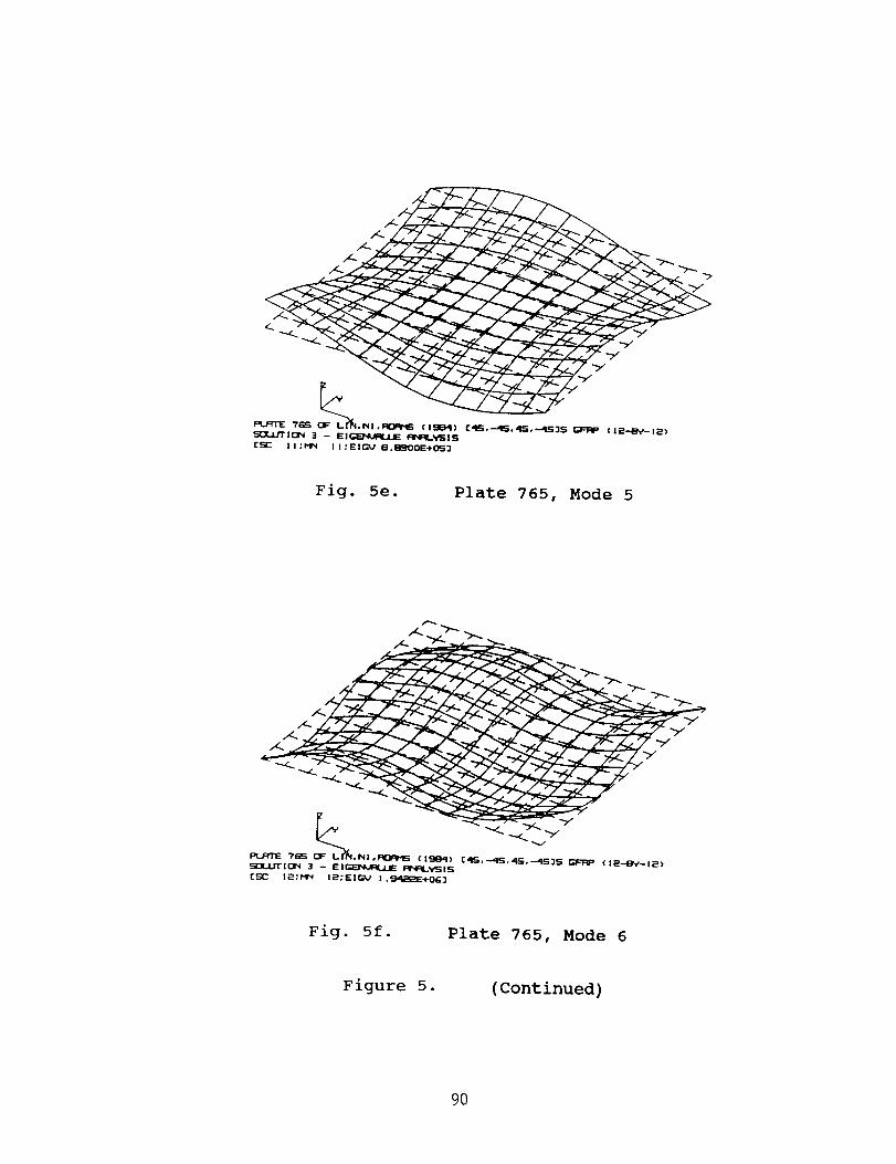
"7
"7"
Pu=r]'E "#'_ [_,IU ,INI,FI:]IW'E (19B41) C'IIS,--41So_I_,-41SlS Gacl:lP (I;_--4SY-12)
SOL,L.VrI(JI"_ 3 - EIGE)%WIFILIJE lel'l:lUl_lS{tar- I I :FIN I 1 :IEIGV e. miqO01E+0S ]
Fig. 5e. Plate 765, Mode 5
PLFITE ?G5 I_IF L.?_fiq,Fllo_ (19E_q) r_qL_,--4FJ,4S,-._IS'}S _ (12--B'_--1;_)SDLJJrrlC:IIN 3 -- EIGi_'qt_I:I..J.IE ISfqRL%r"_15CE 12:Pl_ 12:EIl{_J I ._4=_E_E*Oi_:l
Fig. 5f. Plate 765, Mode 6
Figure 5. (Continued)
9O

?llS OF I..fN,Nl,lql:/:tS (Ig84) [O,SO,4S,_)S GFI:IP (ILS-.BV-12)cJ3.UTIO_l i -- EIGB_IJi=U.E P/_iq-_SlSrSiC "/':m 7': I[ IGIJ El. "T?4UE4'04:]
Fig. 6a. Plate 769, Mode 1
PLqTE "Tim ,NIoII"EYI'IS (IS84) ro,90,4S,..=qS:]S GF'IRP (IL:_B'_I_)SOL.UTI[_ ]i -- Ei(;S'_IPLJJE Iqr4RL.%SilSrc_' 8: /'IN 8: EJGIJ i_. II(_?IE+OS3
Fig 6b. Plate 769, Mode 2
Figure 6. NASTRAN-computed eigenmodes for plate 769
91
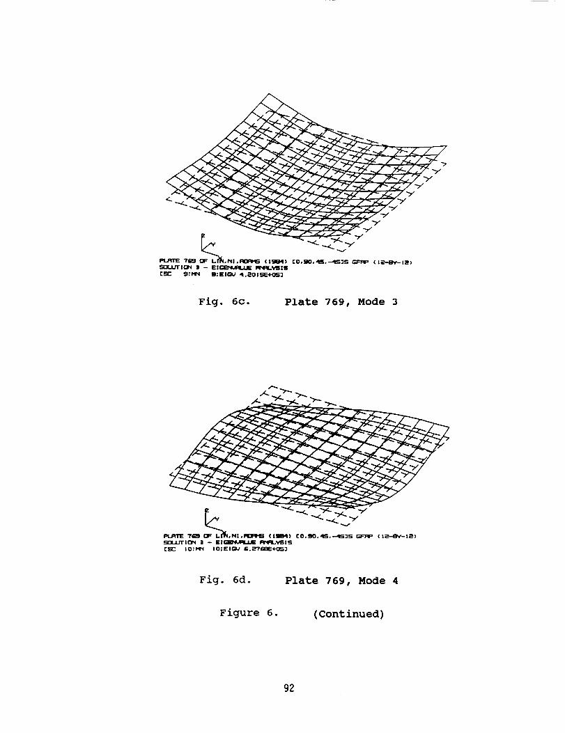
kR..RI"E 7_ ,Nl,lql_1_ (IgB4) [O,90,al6,.-a;S'_S _F'RP (I_-.18_--I_)Sl3LLfflart 3 - EIGS_,4_LLE F'r4_L._5IS
CS;C: g:m g; Eli_J ai.i_01SE+0S]
Fig. 6c. Plate 769, Mode 3
PL,qTE 7_ OF LIIq, NI,PK]PP6 (IgBq) [0,90,4S,--4515 GI=FIP (IE--EY--IE)
S_L,LJTli:_ : -- EIIG_'_R:L,t.JE I:N:4.,_iSCq'" I O: PIr'i I 0:EI_J G .L:"/'GBE+OS 3
Fig. 6d. Plate 769, Mode 4
Figure 6. (Continued)
92

PS.J:qTE "r_q OF L_4°NI,In_uf'6 (1994) CO,90,,qS,--dIS2S G;FIqF' (I2--BY-12)
Sii:]ULJI"I(31 3 -- EIG_Xq.LIE lq'41_.YSISCca'" i I :Pr4 i i :EIQJ 7 . 4704E+OG)
Fig. 6e. Plate 769, Mode 5
PL,RTE 769 .Nl.lq)qt5 (lSO4) [0.90,qS,-'qS'IS GFIqP (IE'-EY--IE)
SOLUTION 3 - EIGB_,4c_/_LJE fq_lqL.*_;15Cc_" 12:Mr4 I;_: EI(_J a . (]S'qbdE4"OG "t
Fig. 6f. Plate 769, Mode 6
Figure 6. (Continued)
93

I<
Ulfl I:s'I.,FTI'_'! _ l..lP.l,_41,1Cll_C:leq5 I"(Qo-."GO, _ (I,_.-Bq'--I_)
(c:r" 7;MI_ 7:E|_ 3 , 7353E+Q_ "1
Fig. 7a. Plate 771, Mode 1
ImUmTE_ "4" _z" _"V|S I OF I.II_I,NI,I_Q_I+6 [(O.'-t_O.GO)|)S I;F'RP (t+la)
SQI/2TIO_I _I -- EI_"_.I_IJ.E IqSlqI.YBIS
(so S:_ s:E_ s.Tal tE+0s]
Fig 7b. Plate 771, Mode 2
Figure 7. NASTRAN-computed eigenmodes for plate 771
94

JD4 UIB _ _11_! OF I.lfl.l_lolql_IG [(O,-iO,iO)|]S _ (IL :_lh_l|)UDUJTII_ • -- EIGm_AnLJJ Iq_/.YSlS
CC_ gl- 14N g: EI_J I. 4a_E_Q_3
Fig. 7c. Plate 771, Mode 3
JD4 rIO PL,IPrI"IE_I _ I-IN, NI.PI_PI'q_ r(O,-GO,GO)E]S _ (IL w-i_lL-18)
Si[_lJTIO'q • - EIG_It.AqL.LE Ilqql_qqBISCIt' 10:m SO:EI_ E. ]IG"TEE+OG'J
Fig. 7d. Plate 771, Mode 4
Figure 7. (Continued)
95

VIe I:_qTE_'_I DI = L.IN,NI,IqT@6 r(0,--G00_)_U6 GFIqP (IL'_-O_--It)
liRX.LrI'IO_¢ ]1 -- E|I_FJPILJJE PNqL._ISCm" I I "Mrq 11;EI_ _.'r'F i (E4-OG]
Fig. 7e. Plate 771, Mode 5
JO4 v:,:, Pt.JqnE_, OF c.i_.Ni.r_'.es cco._¢_.o)_Js _p (ie-ev-ta)
S[3L,i.fflON ] -- EIGB%_qLLE liiNFL%'SlSCc='" la;t'11N IE:EIGIJ "/'. IdJqiE+0¢;'l
Fig. 7f. Plate 771, Mode 6
Figure 7. (Continued)
96

Fig. 8a. Plate 762, Mode 1
JO'l VlB OF LIN, NIoKI:I'6 r(O)B3 I::FRP (le--I_h-i;e)¢Joi.J.Jlrll:_l ! - EIGB_ARI..LE FIPI_IS
Fig 8b. Plate 762, Mode 2
Figure 8. NASTRAN-computed eigenmodes for plate 762
97

v
JC_ UIB DF' I.IN,NI,RI:]RI'lS 1"(0)83 _ (12--B_-IE)
_lOrt 3 - EI(;B_,_dL,LE RNFL_._IS
Fig. 8c. Plate 762, Mode 3
_VIBPL.FqTE_C]F LIN, Ni,_ C(0 ILa-BV_te)
5C]L2.JTIc]r_ 3 -- EI(;E_4,A_J.Elur, FL'_SlS
Fig. 8d. Plate 762, Mode 4
Figure 8. (Continued)
98

Fig. 8e. Plate 762, Mode 5
rIO OF LIN, Ni,_ [(0)8] _ (liFOIsl_-I ll)S[31.1./T,¢_ ]i -- EIGB_k4q[.I.E Iq'_I._ISlS
Fig. 8f. Plate 762, Mode 6
Figure 8. (Continued)
99

N92-24330
A CASE OF POOR SUBSTRUCTURE DIAGNOSTICS
Thomas G. Butler
BUTLER ANALYSES
Substructuring is a powerful tool. As with any powerful
tool the options for managing a Job are legion. On the other
hand, the NASTRAN Manuals in the Substructurlng area are all
geared toward instant success, but the solution paths are fraught
with many traps for human error. Thus, the probability of suf-
fering a fatal abort is high. In such circumstances, the neces-
sity for diagnostics that are user friendly is paramount. This
paper is written in the spirit of improving the diagnostics as
well as the documentation in one area where the author felt he
was backed into a blind corner as a result of his having com-
mitted a data oversight. This topic will be aired by referring
to an analysis of a particular structure.
The structure, under discussion, used a number of local
coordinate systems that simplified the preparation of input data.
The principal features of this problem are introduced Dy refer-
ence to a series of figures.
Figure 1 illustrates a PILOT model of the basic component
substructure of a full scale structure. This pilot model
was used to explore the error that developed in the true
structure. In preparation for the investigation into the
difficulty that was encountered during a "COMBINE" operation,
the pilot basic was cloned 4 times into CLONA, CLONB, CLONC
100

SUBSTRUCTURE DIAGNOSTICS
and CLOND.
Figure 2 tabulates the bulk data for the 5 coordinate systems
that were used in the Dasic component. Coordinate system "5"
is cylindrical and was used for its core. Coordinate systems
"50, 60, 70 & 80" are rectangular and were used [or the four
arms with their local X axes pointing outward at zero de-
grees, 90, 180 and 270 respectively. Each clone retained its
own copy of the set of five local coordinate systems. Thus,
the Substructure Operating File (SOF) at this point had a
complement of 5 x 5 = 25 coordinate systems to catalog. The
multiplicity of coordinate systems was at the root of the
fatal error which erupted.
Figure 3 illustrates two separate "COMBINE" operations
amongst the substructures. In the first "COMBINE", point 51
of P/S CLONC Joins with point 71 of P/S CLOND. In the second1
"COMBINE", point 61 of P/S BASE joins with point 81 of P/S
CLONA, while point 61 of P/S CLONA joins with point 81 of P/S
CLONB.
During the subsequent linking of substructures, the points that
were combined each had their own local coordinate systems. Well
this doesn't seem to be a problem, because NASTRAN has a wonder-
ful module called CSTM (Coordinate System Transformation Matrix)
which keeps track of all transformations amongst a host of coor-
dinate systems. So the user is disarmed into thinking that
I. The abbreviation P/S, meaning pseudo-structure, is used as a
generic term for any number of different kinds of substructures:
basic, or clones, or condensations, or combined.
i01

SUBSTRUCTUREDIAGNOSTICS
NASTRAN can handle anything dealing with coordinates. This was
especially true in this case, because, just prior to the abort
being described here, a mistake in translating one of the cloned
structures was corrected in response to a diagnostic message that
declared that points, which were targeted to be joined, were not
within tolerance. The error was that one of the translations,
defined on a "TRANS" card was off by an eighth of an inch. After
the correction a message was issued declaring that all points in
the "COMBINE" operation were within tolerance. So the reaction
to a subsequent message to the effect that the local coordinate
systems were incompatible seemed ridiculous, because NASTRAN had
no difficulty in locating the points in space and in pronouncing
that they were within tolerance with the coordinate systems that
were corrected.
As it turned out there are a number of different coor-
dinate systmes that have to be dealt with here, and the "TRANS"
set that was Just corrected - though at first suspected - was not
at the hub of the problem. The problem arises not in the align-
ment, which the TRANS coordinates deal with, but in the sub-
sequent mating, which depends of the local DISPLACEMENT coor-
dinates of points that are being brought together.
As a matter of general substructuring principle, when a
group of substructures is assembled, any place where parts are
linked can involve contributions from 2 or more individuals. At
any such place the set of points are merged into a resultant
single point. What is not told in the manuals is that the resul-
tant point needs to refer to just one coordinate system. If all
of the merging points refer to a common coordinate system, there
is no problem. But, when each point has its own local displace-
ment coordinate system, NASTRAN aborts and issues a message #6528
102

SUBSTRUCTURE DIAGNOSTICS
saying that incompatible local coordinate systems have been
found. But if the user thinks that the problem has Just been
corrected, the characterization of the coordinates in message
#6528 as being "incompatible" doesn't make sense and he becomes
convinced that there must be a bug in NASTRAN and the user is to
be absolved of blame. Hls certitude of blamelessness is further
reenforced by the details that are supplied wlth the diagnostic
message. The text of the complete message, shown in Figure 4,
refers to local coordinate systems I and i0. But if you look at
Figure 2, you can verify that no coordinate system was numbered 1
or i0. This seems to further corroborate that NASTRAN got some
tables mixed up and is in need of having a bug straightened out.
Gordon Chan of the UNISYS Support Group came to my rescue
and published the transformation matrices for the coordinate
systems that were involved. The reasnn that NAS_T,'AN aborted was
rluL buc_u_ u£ an error in the code. It deliberately compared
the local coordinates at the combining point and found that one
pair of signs was aligned while the signs of two other axes were
of opposite in sign. The message referring to coordinate
systems resulted from a partially completed execution of the
COMBINE command. It had reassinged coordinate system ID's in
terms of its own internal bookkeeping system, Dut it phrased the
diagnostic in terms of its own scheme of ID's. Unformtunately,
that part of its completed operation was never output, because of
the abortion, so the diagnostic which was trying to be helpful
was confusing the situation even further. However, NASTRAN
appeared to be operating properly.
Double checking of coordinate systems 50 through 80 found
them to be error free. As a further check, the manual method was
103

SUBSTRUCTURE DIAGNOSTICS
compared to the automatic method of combining. The same diagnos-
tic regarding incompatible local coordinates showed up in this
automatic trial as well, but this time referred to pairs of
coorainates with other sets of strange identifications; i.e. 2 &
9 and 7 & 14. That diagnostic is shown in Figure 5. Finally a
vague, misty fragment seemed to Kindle in the back of my brain
that had something to do with the data card called "GTRAN'. I
pored over the Substructure Section of Chapter 1 of the User's
Manual to uncover a hint on the use of GTRAN. No help. Nor was
the Theoretical Manual any assistance. Figure 1 shows that in
the example of the manual COMBINE, points 51 and 71 refer to
coordinate systems 50 & 70 respectively. NASTRAN finds that
these two systems do not align with each other and so both cannot
be allowed to represent that point after a merge. The situation
must be reconciled and NASTRAN needs guidance from the user. The
avenue by which the user exerts his preference is through the use
of GTRAN. The bulk data explanation of GTRAN left many unanswer-
ed questions. The only thing left to do was to resort to the old
"black Dox" method of finding out how it behaved. GTRAN was
tried out under its options. One option is to refer all connect-
ing points to the overall basic system, and the other is to refer
them to the system defined by the TRANS entry. Both worked!
Figure 6 shows an excerpt of the output from a successful manual
run using GTRAN. It repeats the message about points within
tolerance, then gives the tabulation of the resulting points
after the COMBINE operation, showing those degrees of freedom
that were merged into a single point. This connectivity summary
does not, however, refer to any coordlnate system. Coordinate ID
information is published subsequently in the BGSS. In this case
the BGSS shows that it was arbitrated by referring both points to
the "0" system (the overall basic).
104

SUBSTRUCTURE DIAGNOSTICS
Figure 7 is an excerpt of a summary of connectivities for
the automatic COMBINE case after a proper use of GTRAN. It shows
a similar set of connections as in the manual case but amongst
BASE, CLONA, and CLONB.
There were many unhappy features relating to documenta-
tion in this encounter: (i) the diagnostic itself, (2) the
explanation of the diagnostic in Chapter 6, (3) the guide to
modeling in Chapter i, (4) the explanatory notes in the bulk
data, and (5) the Theoretical Manual. It is incumbent upon the
manuals to acquaint the user with what its needs are so that he
can supply necessary data. But in this instance the documenta-
tion gave NO hint of how NASTRAN operated internally, so the user
was set adrift by a diagnostic that impugns his data as INCOMPAT-
IBLE. For all he knew NASTRAN had some sort of internal default
to meet the arbitration needs. Without the help of documenta-
tion, the user must look into the code to find out what NASTRAN
is doing in subroutine "COMBI". He does not know from the above
documentary sources whether NASTRAN takes a default when not
supplied wlth specific direction or aborts. The situation is
this. NASTRAN first determines that the points that it is di-
rected to llnk are collocated. This can be done by temporarily
transforming all locations to the overall basic system. But now
when it wants to trim all connecting points to a single point, it
must assign some coordinate system to that resulting point. But
which one? Dave Hertlng and the savants that helped him with the
architecture of SUBSTRUCTURING were aware of the problem and
provided for it with the GTRAN card. But as is often the case
with programming, the documentation did not coach the user into
anticipating the need to guide NASTRAN in the assignment of a
coordinate system to a common point.
I05

SUBSTRUCTURE DIAGNOSTICS
Rather than overcome the obstacle with the provision of a
GTRAN card and then to continue with the analysis of the struc-
ture only, I chose to share this experience at the Colloquium and
to volunteer a supplement to the documentation so that any
subsequent user can be well guided when he encounters message
#6528. Figure 8 shows the recommended diagnostic message.
Figure 9 shows the recommended supplement to the "COMBINE"
section of Chapter 1 on modeling with substructures, and in
Chapter 6 on explanation of diagnostics. No suggestions are
offered for the Theoretical Manual, because it is currently
awaiting a major revision.
I extend my deep appreciation to Gordon Chan for his help
in unearthing this problem and for his modification of the dlaq-
nostic message in the code. The new release will have the re-
vised diagnostic message. In addition Gordon Chan added a print-
out of the transformation matrices of the coordinate systems that
are indicted.
My hope is that this small effort will save future users
much time and frustration when faced with an unsuccessful COMBINE
operation in their substructuring work.
106

SUBSTRUCTURE DIAGNOSTICS
Figure i. Plot of Basic Component BASE of Pilot Model.
107

SUBSTRUCTURE DIAGNOSTICS
CORD2C 5 0 0.0 0.0 0.0 0.0 0.0 10.0
+CYLN 10.0 0.0 10.0
CORD2R 50 0 I0.0 0.0 I0.0 i0.0 -I0.0 I0.0
+RAYO 20.0 -i0.0 I0.0
CORD2R 60 0 0.0 I0.0 I0.0 I0.0 i0.0 i0.0
+RAYgO I0.0 20.0 I0.0
CORD2R 70 0 -I0.0 0.0 I0.0 -I0.0 I0.0 I0.0
+RAY180 -20.0 I0.0 I0.0
CORD2R 80 0 0.0 -I0.0 i0.0 -I0.0 -I0.0 I0.0
+RAY270 -I0.0 -20.0 I0.0
+CYLN
+RAYO
+RAY90
+RAY18
+RAY27
Figure 2. Coordinate Systems in Component BASE
1Q8

SUBSTRUCTURE DIAGNOSTICS
7/
|
4O
71
TRANS
8o
Figure 3. Connection Diagram of Two COMBINE Operations
I09

SUBSTRUCTURE DIAGNOSTICS
USER INFORMATION MESSAGE 6516,
ALL MANUAL CONNECTIONS SPECIFIED ARE
ALLOWABLE WITH RESPECT TO TOLER.
USER FATAL MESSAGE 6528,
INCOMPATABLE LOCAL COORDINATE SYSTEMS
HAVE BEEN FOUND. CONNECTION OF POINTS
IS IMPOSSIBLE, SUMMARY FOLLOWS.
**************************************
THE FOLLOWING MISMATCHED LOCAL COORDINATE
SYSTEMS (CSTM) HAVE BEEN FOUND FOR
LOCAL COORDINATE SYSTEM ID NO.
PSEUDOSTRUCTURE ID NO. 1
INTERNAL POINT NO. 2
***************************************
LOCAL COORDINATE SYSTEM ID NO.
PSEUDOSTRUCTURE ID NO. 2
INTERNAL POINT NO. 14
USER FATAL MESSAGE 6537, MODULE COMB1TERMINATING DUE TO ABOVE ERRORS.
I0
Figure 4. Diagnostic From Abort of Manual COMBINE
110
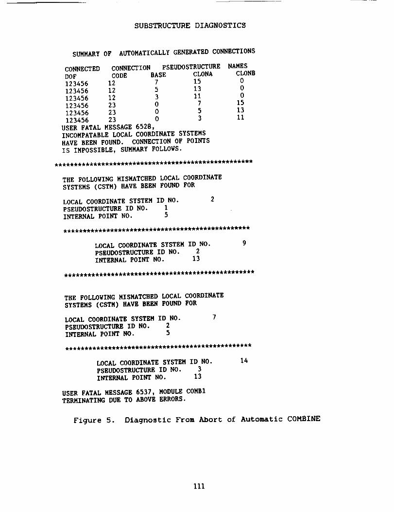
SUBSTRUCTURE DIAGNOSTICS
SUMMARY OF AUTOMATICALLY GENERATED CONNECTIONS
CONNECTED CONNECTION PSEUDOSTRUCTURE NAMES
DOF CODE BASE CLONA CLONB
123456 12 7 15 0
123456 12 5 13 0
123456 12 3 II 0
123456 23 0 7 15
123456 23 0 5 13123456 23 0 3 Ii
USER FATAL MESSAGE 6528,
INCOMPATABLE LOCAL COORDINATE SYSTEMS
HAVE BEEN FOUND. CONNECTION OF POINTS
IS IMPOSSIBLE, SUMMARY FOLLOWS.
THE FOLLOWING MISMATCHED LOCAL COORDINATE
SYSTEMS (CSTM) HAVE BEEN FOUND FOR
LOCAL COORDINATE SYSTEM ID NO.
PSEUDOSTRUCTURE ID NO. 1
INTERNAL POINT NO. 5
2
************************************************
LOCAL COORDINATE SYSTEM ID NO.
PSEUDOSTRUCTURE ID NO. 2
INTERNAL POINT NO. 13
THE FOLLOWING MISMATCHED LOCAL COORDINATE
SYSTEMS (CSTM) HAVE BEEN FOUND FOR
LOCAL COORDINATE SYSTEM ID NO.
PSEUDOSTRUCTURE ID NO. 2
INTERNAL POINT NO. 5
************************************************
LOCAL COORDINATE SYSTEM ID NO.
PSEUDOSTRUCTURE ID NO. 3
INTERNAL POINT NO. 13
14
USER FATAL MESSAGE 6537, MODULE COMB1
TERMINATING DUE TO ABOVE ERRORS.
Figure 5. Diagnostic From Abort of Automatic COMBINE
III

SUBSTRUCTURE DIAGNOSTICS
USER INFORMATION MESSAGE 6516,ALL MANUAL CONNECTIONS SPECIFIED ARE
ALLOWABLE WITH RESPECT TO TOLER.
SUMMARY OF PSEUDOSTRUCTURE CONNECTIVITIES
INTERNAL INTERNAL DEGREES OF
POINT NO DOF NO FREEDOM
PSEUDOSTRUCTURE NAMES
CLONC CLOND
16 89 123456 CLONC
72
17 95 13 CLONC CLOND
51 71
18 97 123456 CLOND
51
Figure 6
Summary of Connectivities After GTRAN Use in Manual COMBINE
112

SUBSTRUCTURE DIAGNOSTICS
SUMMARY OF AUTOMATICALLY GENERATED CONNECTIONS
CONNECTED CONNECTION PSEUDOSTRUCTUREDOF CODE BASE CLONA
123456 12 7 15123456 12 5 13
123456 12 3 11123456 23 0 7123456 23 0 5
123456 23 0 3
NAMESCLONB0
00
1513
11
SUMMARY OF PSEUDOSTRUCTURE CONNECTIVITIES
INTERNAL INTERNAL DEGREES OF *POINT NO DOF NO FREEDOM BASE
PSEUDOSTRUCTURE NAMES
CLONA CLONB
16 89 123456 BASE72
17 95 13 BASE CLONA
61 81
18 97 123456 CLONA52
33 183 123456 CLONA2
34 189 13 CLONA CLONB61 81
35 191 123456 CLONB52
Figure 7
Summary of Connectlvltles After GTRAN Use in Automatic COMBINE
113

SUBSTRUCTURE DIAGNOSTICS
USER FATAL MESSAGE 6528
INCOMPATABLE LOCAL COORDINATE SYSTEMS HAVE BEEN FOUND. COMPLETTION OF
CONNECTION IS IMPOSSIBLE. SUGGEST USE OF "GTRAN". SUMMARY IN TERMS OF
JUST-FORMED INTERNAL FREEDOMS AND INTERNAL COORDINATE SYSTEM ID'S PER THE
EQSS & BGSS FOLLOW:
Figure 8. Revised Fatal Diagnostic Message 6528
114

SUBSTRUCTURE DIAGNOSTICS
USER' S MANUAL CHAPTER I.
ADD THE FOLLOWING TEXT TO SUPPLEMENT THE TOPIC OF THE "COMBINE" OPERATION ON
SUBSTRUCTURING IN THE NASTRAN USER'S MANUAL, PAGE 1.10-39 (14 LINES UP FROM
THE BOTTOM OF THE PAGE.
WHEN POINTS ARE ALIGNED FOR COMBINING AFTER A TRANSLATION AND/OR ROTATION OF
COMPONENTS, THEY BECOME A SINGLE POINT UPON LINKING. IF THE POINTS ABOUT TO
BE CONNECTED REFER TO DIFFERENT LOCAL COORDINATE SYSTEMS, THE SUBSTRUCTUREROUTINE "COMB1" DOES NOT IMPOSE A DEFAULT CORRDINATE SYSTEM FOR THE POINT.
SUCH A SITUATION MUST BE ANTICIPATED BY THE ANALYST TO AVOID A FATAL ABORTION.
THE ANALYST CAN ASSIGN A DISPLACEMENT COORDIANTE SYSTEM TO THE RESULTING POINT
THROUGH THE USE OF THE GTRAN CARD. IT OFFERS 3 OPTIONS: (I) TRANSFORM TO THE
OVERALL BASIC SYSTEM, (2) NO TRANSFORMATION, AND (3) TRANSFORM TO THE COORDI-NATE SYSTEM WHICH WAS DEFINED ON THE SELECTED "TRAMS" CARD.
USER'S MANUAL CHAPTER 6.
ADD THE FOLLOWING TEXT AFTER THE FIRST SENTENCE OF DIAGNOSTIC MESSAGE 6528.
EACH POINT IS CARRYING ITS OWN LOCAL COORDINATE SYSTEM INTO THE "COMBINE'D"
POINT AND THEY HAVE BEEN FOUND TO BE DIFFERENTLY ALIGNED_ I.E.
INCOMPATABLE. THE USER IS REOUIRED TO ARBITRATE BETWEEN THE COMPETING
LOCAL COORDINATE SYSTEMS. HE IS ADVISED TO CONSIDER USING ONE/OR SEVERAL
"GTRAN" CARDS. (SEE PAGE 1.10-39 OF THE USER'S MANUAL.) HE IS FURTHER
ADVISED TO "DESTROY" THE PSEUDO-STRUCTURE DEFINED IN THE COMBINE OPERATIONIN ORDER TO REMOVE ANY PARTIALLY COMPLETED "COMBINE" DATA FROM THE SOF
(SUBSTRUCTURE OPERATING FILE), BEFORE RERUNNING THE "COMBINE" OPERATION.
Figure 9. Supplements to Documents in USER'S Manual
115

N92-24331
ALTERNATIVE METHODS TO MODEL FRICTIONAL
CONTACT SURFACES USING NASTRAN
Joseph Hoang
GE Goverment Services, Houston, Texas
SUMMARY
Elongated (slotted) holes have been used extensively for the integration
of equipment into Spacelab racks. In the past, this type of interface has been
modelled assuming that (1) there is no slippage between contact surfaces, or
(il) there is no load transfer in the direction of the slot. Since the contact sur-
faces are bolted together, the contact friction provides a load path determined
by the normal applied force (bolt preload) and the coefficient of friction. This
paper examines three alternate methods that utilise spring elements, exter-
nally applied couples, and stress dependent elements to model the contacted
surfaces. Results of these methods are compared with results obtained from
methods that use GAP elements and rigid elements.
INTRODUCTION
Elongated holes have been used in the design of Spacdab Experiment Equipment
mounting provisions. This type of joint is employed where large tolerances are allowed
in one direction of the hole for the ease of integration. A simple way to model these
interfaces is to use RIGID elements with the assumption that two connecting grid points
are not moving against each other when loads are applied. Another common method is to
use RIGID elements with the degrees of freedom associated with the longitudinal direction
of the elongated hole released. When using this method, it is assumed that the joint did
not carry load in its slotted direction.
Due to the assumption involved, neither method yields realistic results. GAP dements
have been used to achieve better results. However, when large numbers of GAP dements
are used in a complex model, an unreasonably large amount of computer processing time
is required to solve the system and, hence, is not economical or practical.
In this paper, three alternative methods are investigated. The first method employs
a spring element with a spring rate equal to the maximum load at the connection divided
by the gap length. By using a spring element at the connection, the nonlinear frictional
116

force developed at the gap is replaced by a spring force that increases proportionally with
gap distance. The second method used an externally applied couple to represent the
frictional forces at the two contacted surfaces. This method creates a local realization of
frictional forces when two grid points, representing two contacted surfaces, move against
each other. In the third method, two contacted surfaces are connected by elements with
stress-dependent material properties. The piecewise linear static analysis rigid format is
ultilized to solve element forces at these elements.
A simple stowage container and four supporting columns were developed to represent
a typical installation in a Spacelab rack. The container was integrated on supporting
columns using the above methods. The models were run on a SUN workstation using
CSA/NASTRAN. The results obtained from each method were then compared.
THEORY AND BACKGROUND
Figure la shows a typical elongated hole and Figure lb shows force vs. relative
displacement of an elongated hole. The force vs. displacement curves of other elements
are show_,,_ i_ _;_,:_,'_ 2 through 7.
From inspection, the stress dependent material element is the more appropriate ele-
ment to simulate elongated hole behavior because the GAP element, spring element and
coupled element would generate some error. A rigid element with all three translational
degrees of freedom coupled (R123) should be used only when the frictional force is greater
than the force at the connection. A rigid element with degrees of freedom associated with
the longitudinal direction of the hole released (R23) should be used when, the frictional
force and the displacement in elongated direction are small.
117

Fig la Typical elongated hole Fig lb
y
orcevs displacement of elongated hole
Fig 2
v
orcevs displacement of R123 element Fig 3 Force
Iiii,ii_
iiiii--
vs displacement of R23 element
Iiiiiiii_
n.,iii-
Fig 4 Forcevs displacement of couple element
v
Fig 5 Fdrcevs displacement or sor_ngelement
118

Fig. 6 Force
r
vs, displacement of GAP element Fig 7
v
orcevs displacemen[ of nonlinear element
1002 I004
1013 13
06 1008
1037 37 1017 17 20 1020
1001
4144 1044
1005 1007
Fig. 8 Plot of test subject a simple box and four supported columns
119

ANALYSIS AND RESULTS
A simple box is constructed using QUAD2 elements. It is supported by four columns
which were modelled using BAR elements. A plot of the structure is shown in Figure 8.
In the rear, the box is mounted on two rear columns at grid points 13, 24, 37, and 48
using rigid elements with all three translational degrees of freedom coupled. In front, the
box is mounted to the front left column at grid points 17 and 41 and to the front right
column at grid points 20, and 44, using a different integrating method. Gravitational loads
varying from 0.2g to 4.0g are applied to the model in the X-direction, which is parallel to
the slotted direction.
The material and properties of QUAD2 and BAR elements are chosen such that the
box is heavier and more flexible than the columns. Since the columns are much stiffer than
the box, displacement of the grid point on the column is small as compared to displacement
of the grid point on the box. Displacement of the rear panel is closed to the displacement
of rear columns because the rear panel interface points are mounted to the rear columns
by rigid elements with aJ] three translational degrees of freedom coupled. However, at
the frull_ panel, the relative displacement of front panel and front columns are greatly
dependent on the type of connecting elements used. It should also be noted that the single
point constraint forces developed at the front columns are also dependent on the amount
of load that has been transfered to the columns through the front connecting elements.
Properties of each type of connecting element are chosen in such a way that its de-
formation can follow the elongated hole displacement curve as close as possible. The gap
length and frictional force of the contacting surface were chosen arbitrarily at 0.5 inches
and 15.0 lbs respectively.
Displacement of the left front interfaces (grid points 17 and 41 were identical and
were tabulated in Table 1). The single point constraint force of the left front column (grid
points 1005 and 1006) are tabulated in Table 2. Table 3 shows the displacement of the
right front interfaces (grid points 20, and 44) while Table 4 shows a single point constraint
force of the right front column (grid points 1007 and 1008).
120

_,..1
0U
It.,0
E-,
_0O_
E.,_.U
r.l
[JlE
U
,<,-1
,-4
,,n
ooIllllflillllllllllgl
_ _000000000000000000000000.00000.0000 ....
IIIIIIIIIIIIIIIIIIII
_ ._ 0 _
00000°00000000.0 ....
O0 C_O0000000000000000
I I I I ! I I f i I I I I ,+ '+ + + + 4- -I-_,1M M M Ill I_ M ¢ll bll Ill] [,] I_ [11 _1 r_l M M M r_ _1
o • • • • o • • _ • • , o o , . .
+111111111t+++++++++
O" _ _ 0 _ _
0.o00.o°_oo0000oo0o.o
IIIlll
IIIII@++@+++++++++++
• ..... oooooo,, ......
o_____oo oo ooIIIIIIIIIIllllllllll
.... 0_.000000 .......
o
<
oo
F,
0
'_0
O_
0
!
I-4
0
M
E_
I+++++++++++++++++++HHHHHHHHHHHHHHHHHHHH
_ _ _ _0 0
0_0o°ooo°0oo00o0o000
00000000000000000000+÷÷÷÷+÷+÷÷÷÷÷÷÷÷÷÷++
0000000.000 ....... 00
?T_??7777777??7??77T
++++++++++++++++++@+_MM_M_M_MM_MM_MM_M
00 ...... 0.o0o00..o0o
7?7_?T77777777777777
++++++++++++++++++++M_M_MM_MMMMM_H_M_
o,o°...oooooooooooo°
?????????????7777777
__oooooo__ooooooIII;11+++++++++++÷++
oo°.o00o..o..0,000o0
77T_?T777777,77, , , ,7
+++++++++++÷++÷+++++
MMMMM_MM_M_BMMMM_BM
........ o o • ...... , o .
_3
0,..1
o.,.o.o,o..o .... ,o..
oooo____ 0
.... .0,.0,.,.o,,.o,,
oooo____
121

_ooooooooooooooooooo
_3
c)r_
oooooooooooooooooooo;;ll;lllll;lllllll;I
__mmmmmmmmmmmm
oo3333o oo 3333__I;lllllllllll+++++÷÷
_oo____ o
0
0
0
t)
L)
In
C:
+llllllllll+++++++++
Illlll
.......... , .........
r_
L9
H
Ul
o
0
I
M
_4
I+++++++++++++++++++
IIIIII I I
+++++++++++++++++÷÷÷
• ° ............. , , , , °
7_TTT_7 ............
++++++++++++++++++++
777777_7 ........ 7-_
IIIII1++++++++++++++
.°°.,0. ........ 0.°..
_TT_T_7 ............
÷÷++÷÷÷++÷++++++++÷+
• • . ...... , ....... ° • .
_ .............. ° .....
122

DISCUSION
Examination of the displacement of the left and right front panels of the box and the
load distribution over four supporting columns indicates that types R123 and 1123 are the
two extreme cases. For rigid R123 types, the load was distributed evenly over four columns;
meanwhile, for rigid R23 types, the load was carried by the rear columns only, and the
box acts as a cantilever beam. The exact load distribution pattern is somewhere between
the boundary established by these two types of connections. With finer load increments,
the displacement curve of a stress dependent material element can be made to match the
displacement curve of an elongated hole and, therefore, used as a reference to evaluate
performance of other types of connections.
In general, static analysis with GAP elements and piecewise linear analysis employ
an iterative scheme for solution. ,,They are costly to run especially when models become
complex. For the problem at hand, the GAP element did not yield a corrected solution
when under tension load, meanwhile, stress dependent material elements did not perform
well when under compression. Therefore, these two types of elements were not suitable for
tuudel with multiple loading cases where the directions of the load at the interfaces are
often unknown.
A couple type connection shows the same characteristics as the R23 type, with the
displacement shifted due to externally applied couple. It is also difficult to use when the
direction of the loads at the connection is unknown. However, the solution can be obtained
with less computing time.
The solution for rigid elements and spring elements always contains some degree of
error, but can be obtained with less computing time, and can be used in problems involv-
ing multiple loading conditions. The spring rate can he adjusted to control the relative
displacement of the two connecting grid points.
RECOMMENDATION
It is recommended that for problems with multiple loading conditions, models should
be run first using R123 type connections. Then, for interfaces that develop forces larger
than the frictional forces of the elongated hole, the type R123 connection should be re-
placed with appropriate spring elements. This methodology yields reasonable results with
minimum computer run time.
123

N92-24332
Hierarchical Tapered Bar Elements
Undergoing Axial Deformation
N. GaneJan and S. K. Thampl
GE Government Services, Houston, Temas
ABSTRACT: A method is described to model the dynamics of tapered
axial bars of various cross sections based on the well-known Cralg/Bamptoncomponent mode synthesis technique. This element is formed in terms ofthe static constraint modes and interface restrained normal modes. This isin contrast with the finite elements as implemented in NASTRAN where theinterface restrained normal modes are neglected. These normal modes arein terms of Bessel functions. Restoration of a few of these modes leads to
higher accuracy with fewer generalized coordinates. The proposed modelsare hierarchical so that all lower order element matrices are embedded in
higher order element matrices. The advantages of this formulation comparedto standard NASTRAN truss element formulation are demonstrated throughsimple numerical examples.
1. Introduction: Tapered bars and beams have high strength to weight ratios as well
as architectural advantages. They are frequently employed to model structures in di-
verse applications, such as ship masts, turbine blades, chimney structures or complex
frame constructions. NASA (Langley) has tested a truss structure which is made from
tapered members to be used in space applications [1]. The technical literature on tapered
beams is indeed vast with a long history [2-10]. Tapered beam finite elements are ei-
ther simple elements (e.g., Lindberg[2], Rouch/Kao[3]) having two degrees of freedom at
each end or higher order elements (e.g., Thomas/Dokumaci[4], To[5]) having more than
four degrees of freedom. Ovunck[6], Avakian/Beskos[7], Gupta[8], Banerjee/Williams[9]
and Spyrakos/Chen[10] have used frequency dependent finite elments in their analysis of
tapered bars. Banerjee/Williams[9] have developed exact dynamic stiffness matrices for
Bernoulli-Euler beams. However the approach in References [6-10] involves the unknown
frequencies of the overall structure. The general framework developed by Engels[ill andapplied in References [12-14] allows for the derivation of hierarchical finite elements for
any type of structural element. This approach does not require the prior knowledge of
system frequencies, thus overcoming the need for an iterative procedure to compute the
structural response. In the present paper, a dynamic finite element model for a certain
class of tapered bars with loads acting only in the axial direction is developed. The ele-
ment matrices are presented in parametric form and can be easily extended to formulate
the finite elments for a wide variety of tapered bars covering most practical cases. The
convergence properties of this dynamic finite element, when compared to the regular finite
element, are examined using numerical examples.
2. Assumed Modes Method: The Lagrangian elastic displacement vector e(z,y, z,t)
for a generic element can be written as the sum of two separate displacement vectors ei
124

and i.
• = ez + i (I)
where e! is a quasi-static displacement vector due to the interface displacements qx and is
expressed as a ]/near combination of static constraint modes _i,
= qz (2)
The second part _ represents the remainder of the total displacement vector e. It is that
part of • which is measured relative to el by an absolute observer. Clearly, _ vanishes
at the ql coordinates and therefore can be expressed as a linear combination of assumed
modes qbwhich are restrained at those qx coordinates
}----@_ (3)
The vector _ represents a set of generalized coordinates to be determined as part of the
solution. One example of _ modes are the normal modes of the element E restrained at the
qx coordinates. It should be stressed that although restrained normal modes have often
unique advantages, they are only one of many possible sets. In fact, _ modes need only be
restricted to admissible functions that vanish at the qx coordinates. Substituting Eqs. (2)
/"}and (3)into Eq. (1) yields
(4)
so that • is written in terms of a linear combination of two sets of assumed modes: (1)
static constraint modes and (2) interface restrained assumed modes. It should be noted
that the representation of • in Eq. (4) is complete in the sense that any degree of accuracy
is theoretically possible as long as enough _ modes are added.
In the standard consistent mass matrix approach, the elastic displacement vector e
over the element is represented as a linear combination of interpolation or shape functions.
In fact, these shape functions are identical to the static constraint modes @I and therefore e
is approximated by el as in Eq. (1). The standard finite element approach therefore totally
neglects the displacement _ in Eq. (1). Ignoring _ leads directly to a deterioration of the
modal content of a typical finite element model. One way to ensure better convergence
to a desired model fidelity is suggested by Eq. (4) and leads to dynamic finite element
models. Instead of totally neglecting the _ displacement, one could retain a limited number
of _ coordinates, thereby improving the mass and force distribution models. Of course,
adding _ coordinates also increases the order of the overall model. However, this approach
has three important advantages: (1) The model converges much faster, i.e., far fewer
degrees of freedom are necessary to attain comparable accuracy; (2) in principle, no further
subdivision of basic elements is necessary, thereby simplifying the finite element grid and
(3) the model is hierarchical and therefore has all the advantages associated with this
property. In addition, these finite element models are directly based on the assumed
modes method which provides a sound theoretical basis.
125

In Reference [11] it is shown that for a linear elastic material, the element kinetic and
potential energies T and V can be written as
T= _q Mq, M= eT_bdm (5)E
V = _q Kq, K = (B_b) TC(B_b) dV (6)
E
in which the matrix C is the material stiffness matrix and B contains the appropriate
partial derivatives in z,y and z. Futhermore, the matrices M and K represent the mass
and stiffness matrices of a generic finite element E. In partitioned form,
M = LMTN MNN J' 0 KNN (7)
where
E E E
KII = /(B¢I)TC(BqbI)dV, KNN = /(B-_)TC(B_)dV
(8)
(9)
and
E E
Note that the KIN partition is always zero, which means that no stiffness coupling exists
between ql and _.
At this point, a few remarks are in order. First, the matrices MII and Kll repre-sent the standard finite element consistent mass and stiffness matrices for the element E.
The consistent mass matrix approach represents in fact a static condensation or Guyan
reduction whereby all noninterface degrees of freedom are eliminated. Secondly, if the in-
terface restrained normal modes are used for the columns of ¢, then the present approach
is identical to the Craig/Bampton component mode synthesis procedure as applied to a
finite element. It should be emphasized that the element E is generic. This means that
the proposed approach is valid, at least in theory, for any type of element. In the present
paper, this general procedure will be applied to the special case of the tapered bars.
3. Tapered Bars: The hierarchical stiffness and mass matrices of the tapered bar are
obtained by solving the governing equations of motion for displacement. Figure (I) repre-
sents linear tapered bar ab with a straight centroidal axis and the directions of the principal
axes being the same for all crossections. The cross sectional area A(z) is given by
(A(z)= Aa l +c (10)
where c = db/d,, - 1 and Ai, dl (i = a, b) denote the cross sectional area and the depth
respectively, c > -1 otherwise the beam tapers to zero between its ends and L is the
length of the bar.
126

Although the formulation is valid for any n > 0, many
practical cases of tapered bars arise when n is one or two, see
Figure (2). If the geometrical properties of the element at both
ends are given, the shape function for n can be derived as
log(Ab/Aa) (11)= log(db/d )
For bars of closed box or I-section of constant width and vary-
ing depth, n is not an integer and will vary slightly from E-
q. (10) at all = other than the two ends. But the deviations
are usually within one percent of the exact values.
L
Figure 1.
Tapered Element
4. Static Constraint Modes: Consider the axial bar element as illustrated in Fig-
ure (1). The bar is assumed to undergo vibration along its own axis and as a rigid body can
only move along that same axis. The interface displacements are defined as qz (t) = u(0, t)
and q2(t) = u(L, t), i.e., qz = [ qz q2 ]T and the displacement vector • is considered to have
only one component, i.e., u. Eq. (4) is therefore written as
m
(12)
(n- I ) t
o
(a) (DJ _c_ (d) (e)
1 i-._In=2)
d
(r] (hi (t) /11_
ELEVATION:
,)t
(all cases) d (I .c)a
PLANS:
(for (b). (el, (ell, (cJ),
(for (a), (f) & (t)) (h) & (Ill(for (e))
l}
Figure 2. Sample Cross Sections
127

The static constraint modes, _bi can be computed from the differential equation for
the axial deformation u at z from end a of the tapered bar,
where E is Young's modulus. Integration of Eq. (13) gives,
(13)
EA(z) d_ =CI (14)
Substituting for A(z) from Eq. (10) and setting _ = 1 4- c_ gives
du CIL 1
d_ EAoc C _
Integrating Eq. (15) again,
(15)
where
CIL
- k--27, f(_) + C_ (16)
1
f(_) ---- (n- I)_ n-1 for n _ 1 (17)
= In _ for n = 1
The appropriate boundary conditions for the computation of static constraint modes are
given by
ql =1, qz=O
ql -- 0, q2 -- 1 (18)
The resulting static constraint modes are
Ol -- f(_) -- f(1 + c) f(1) - f(_) (19)f(1) - f(1 + c)' ¢_ - f(1) - f(l + c)
Note that these constraintmodes are in factthe shape functions used in the stiffnessmatrix
of the tapered bar.
At this point, enough information exists to compute MH and KH from Eqs. (8-9).
Indeed, for the tapered bar, the kinetic and potential energies T and V are given as
L L
T = _ pA(z) dz, Y = _ _ dz0 0
(20)
Substituting Eq. (12)into Eq. (20) gives
L L
0 0
(21)
178

When n - 1, the explicit expressions for KH and MII are defined as
c[11 11] rmlm12]K,, - ': , M. -L 77I'21 171"22
(22)
where
pAaL [-21n2(1 + c)- 21n(1 + c) + c 2 + 2c]roll = 4cln2( 1 + c)
pA, L [(c 2 -t- 2c -I- 2)ln(1 + c) - c2 - 2c] (23)m12 -- Wit21 "" 4ch2(1 + c)
pA, L [2(1 + c)2(ln2(1 + c) - ln(1 + c)) + c2 + 2c]m22 = 4tin2( 1 + c)
The counterpart expression for KH when n _ 1 is given as
KH = EA"c(n-1)(l+c)"-l___)-_-_-1 _ 1 [11 -1]1 (n_l) (24)
The stifness matrix partitions KH and MH for n = 2 are evaluated as
K. = EA,(1 + _) 1 -1 M.- (25)L -1 1 ' 6 l+e 2(1+c) 2
Because of the similarity of the governing equations between axial bars and torsional
shafts, Eq. (25) can be used as the stiffness and consistent mass matrices for tapered shafts
by replacing the wriables Aa, E with Ja, G respectively, where J, is the polar second
moment of area and G is the shear modulus of elasticity. If it is decided that no extra
coordinates are to be retained in Eq. (4), then the procedure can be terminated at this
stage.
5. Interface Restrained Normal Modes: An entire class of hierarchical models can
now be created solely on the basis of choosing the interface restrained assumed modes. In
this paper, the set of interface restrained normal modes is used. The normal modes and
their corresponding frequencies are obtained from solving the eigenvalue problem associ-
ated with the partial differential equation,
_- EA(z) = pA(z) Bt 2 (26)Bz
subjected to the clamped-clamped boundary conditions.
Substituting for A(x) from Eq. (10) and letting _ = 1 + cz/L gives,
_u n t_u pL 2 a_u_ -{- --- --- (27)a__ _ 0_ Ec_ &2
129

For harmonic vibration,
u(_,t) = U(_)sinwt (28)
where t denotes time and w is the circular natural frequency. Eq. (27) is modified using
Eq. (28) as
d 2 U n dU w2 pL 2d_--5- + _ _- + _c2U = 0 (29)
The solution of Eq. (29) when c > 0 is
V(_) = _ _;av- { asz:_ (a_) + BY,_,, (a_)} (30)
where J and Y are Bessel functions of the first and second kind and a = _ V/-_-E.
For the case of n = 2, imposing the clamped-clamped boundary conditions in Eq. (30)
yields the characterstic equation for the tapered bar,
sin ac = 0 (31)
The solution of Eq. (31) is
,, = --_ V p , i= 1,2,...,oo (32)
It is noteworthy that the natural frequencies of the tapered bar with clamped ends for the
case of n = 2 are independent of c and are in fact the same as that of uniform rods. From
Eq. (30), the interface restrained normal modes for n = 2 becomes
¢i = Ci sin(a_ - a) (33)
where the mass normalization constant Ci must satisfy
l+c
1
- 1 (34)
Substituting Eq. (33) into Eq. (34), Ci is determined as
Ci= L(35)
From Eq. (8), the mass matrix partitions are evaluated as
L
MNN = / pA(z)-¢T-_dz = I,o
L
/MtN = [m/i], mji = pA(m)¢i¢idz
0
i = 1,2,...,eo, j = 1,2
(36)
130

with
,nl, = {_. , ,n,i= ,_" 1 + c)(-1)i+1 (37)
When cissettozero,Eqs.(25)and(36)reducetothecaseofuniformbars.Appli-cationof Eq. (33) into Eq. (20) gives the stiffness matrix partitions,
KIN = O, KNN = Diag. [_ w_...] (38)
and _i is given by Eq. (32). It can be seen that the tapered bar element matrices consist
of very simple terms.
6. Demonstration Examples:
6.1 Tapered Cantilever: This first example is concerned
with the cantilevered bar clamped at the right end, see Fig-
ure (3). The pertinent structural parameters are E = 30 ×
106 psi, pg = 0.28391b/in_,A_ = l in2,Ab =4in 2 andL=
72 in.
The characteristic equation of this cantilever is given by
a cos ac + sinac = 0 (39)
Tables (I) and (2) show the number of converged frequencies
to within a given percentage relative error when compared to
the theoretical frequencies from Eq. (39) for different modelorders n.
Figure 3. Cantilever
Note that the bar is subdivided into the requisite number of elements to arrive at the
model order n in the standard finite element method as implemented in CSA-NASTRAN
whereas in the hierarchical finite element model, the number of bar elements is always one
and the requisite interface restrained normal modes are added to arrive at n.
Table 1. Standard Finite Element Method
e
<1%
<5%
< 10%
8 '16 24 32 40
1 3 4 5 6
3 6 8 11 14
4 8 12 16 20
131

Table 2. Hierarchical Finite Element Method
e n
8 16 24 32 40
< 1 % 6 14 23 31 39
< 5 % 7 15 23 31 39
< I0 % 7 15 23 31 39
6.2 Planar Truss: Next, consider the planar single-bay truss
as illustrated in Figure (4). The parameters are the same as
in Section (6.1). The horizontal bar has a uniform cross sec-
tional area of 4 in _. For planar truss elements, the transverse
inertia must be taken into account. This time, however, no
'exact solution' for the frequencies of the structure exists. A
reference solution was obtained in two different ways: (1) by
constructing a highly refined standard finite element model (2)by retaining a large number of normal modes in the hierarchical
model. Both models were refined to the point where no signif-
icant change in the frequencies occured and both the models
produced the same results.Figure 4. Planar Truss
Table (3) lists the frequencies from the hierarchical finite element model when two
normal modes per bar are added (i.e., n = 16) as compared to the reference solution. In
order to achieve comparable results from standard finite element method, each bar has to
be subdivided into five beam elements (i.e., n = 66) and consistent mass matrix has to be
generated within NASTRAN.
Table 3. Frequency Comparisons For Planar Truss
Mode
Number
2
3
5
7
9
11
13
14
16
Reference
Frequency (Hz)
2.606E2
2.999E2
6.958E2
1.467E3
1.757E3
2.141E3
2.889E3
3.049E3
3.382E3
Computed
Frequency (Hz)
2.606E2
2.999E2
6.961E2
1.468E3
1.762E3
2.172E3
2.898E3
3.081E3
3.505E3
Error
%
-1.123E-2
-1.703E-2
-4.763E-2
-1.837E-2
-2.970E-1
-1.432
-3.317E-1
-1.045
-3.622
132

7. Conclusions For the case of tapered bars, it has been demonstated that the modal
synthesis approach, where substructures are assembled to form the overall structure, can
be used at the element level itself. This approach has superior convergence characteristics
and the advantages of hierarchical formulation.
8. References:
.
.
3.
.
.
.
.
,
.
10.
11.
12.
13.
14.
W. L. Heard Jr., H. G. Bush, R. E. Wallsom and J. K. Jensen. A mobile workstation
concept for mechanically aided astronaut assembly of large trusses. NASA Technical
Paper 2108, 1-35 (1983).
G. M. Lindberg. Vibration of nonuniform beams. Aero. Quart. 14,387 (1963).
K. E. Rouch and J. S. Kao. A tapered beam element for rotor dynamics analysis J.
Sou. Vib. 66, 119-140 (1979).
J. Thomas and E. Dokumaci. Improved finite elements for vibration analysis of ta-
pered beams. Aero. Quart. 24, 39-46 (1973).
T. W. S. To. Higher order tapered beam finite elements for vibration analysis. J. Sou.
Vib. 63, 33-50 (1979).
B. Ovunck. Dynamic analysis of frameworks by frequency dependent stiffness matrix
approach. Int. Assoc. Bridge Struct. Engg. Publ. 32, 137-154 (1972).
A. Avakian and D. E. Beskos. Use of dynamic stiffness influence coeffiecients in
vibrations of nonuniform beams, d. Sou. Vib. 47, 292-295 (1976).
A. K. Gupta. Frequency dependent matrices for tapered beams. J. Struct. Div.,
ASCE 112 1-17 (1986).
J. R. Banerjee and F. W. Williams. Exact Bernoulli-Euler dynamic stiffness matrix
for a range of tapered beams. Int. J. Num. Meth. Engg. 21, 2289-2302 (1985).
C. C. Spyrakos and C. I. Chen. Power series expansions of dynamic stiffness matrices
for tapered bars and shafts. Inter. d. Num. Meth. Engg. 30, 259-270 (1990).
R. C. Engels. Reduced order structural modeling techniques for high energy laser
systems. Final report/'or AFWL/ARBM Kirkland, NM (1986).
M. Link, J. Moreno-Barragan and M. Weiland.
using modal synthesis techniques. Proc. Euro.
Bonn (1989).
Derivation of finite clem¢',_ ,_,,¢l_'ls
Forum Aeroe/as. Str. 1)r,.. I)(;IJl_
N. Ganesan and R. C. Engels. Hierarchical Bernoulli-Elder beam tinitc eh'nwllls.
Comp. Struct. (to appear) (1992).
N. Ganesan and R. C. Engels. Timoshenko beam finite elements using assumed modes
method. 2. Sou. Vib. (to appear)(1992).
133

N92-24333
TRANSIENT THERMAL STRESS RECOVERY FOR STRUCTURAL MODELS
William Walls
McDonnell Douglas Space Systems Co.Huntsville Alabama
ABSTRACT
A method for computing transient thermal stress vectors from
temperature vectors is described. The three step procedure
involves the use of NASTRAN to generate an influence coefficient
matrix which relates temperatures to stresses in the structuralmodel. The transient thermal stresses are then recovered and
sorted for maximum and minimum values. Verification data for
the procedure is also provided.
1.0 INTRODUCTION
There are many occasions when the stresses produced by transient
thermal events must be considered. The ascent, on-orbit, and
descent phases of a Spacelab mission produce large temperature
gradients on the Cargo Element. A method for recovering the
thermal stresses produced by these events was developed by the
Structural Analysis Group at McDonnell Douglas Space Systems
Company-Huntsville (MDSSC-HSV), and has been used for more than
six years in Spacelab Evaluation.
Because this method was somewhat unhandy to use, only a limited
number of temperature distributions could be run. These were
generally chosen on the basis of temperature or temperature
difference extremes. Unfortunately, there is no proven
relationship between "worst stresses" and "worst temperatures"
or "worst temperature differences" for the complex models with
which Spacelab has to deal. It was therefore decided to develop
a process that would transform transient temperature vectors
(which are separately calculated) directly into stress vectors
that could then be sorted for maximum and minimum (Max/Min)
values.
Section 2 presents the theory used in the procedure, Section 3
describes the procedure, Section 4 presents verification
results, and Section 5 contains the conclusions.
134

2.0 THEORY
The method described assumes that the thermal strains, and hence
stresses are linearly proportional to the temperatures. The
method, therefore, is not applicable to models having
temperature or stress dependent material properties.
An influence coefficient matrix, [TRAS], to transform the
temperatures at a models n grids into m stresses can be
developed as follows. A temperature of one unit above the
reference is applied to a grid in the model while the remaining
n-i grids are held at the reference temperature. The resulting
m stresses are then recovered. This is repeated for all n grids
in the model. The resulting n sets of stresses are then
assembled as columns to form an m by n influence coefficient
matrix, [TRAS], that can be used to transform temperature
vectors into stress vectors. The transformation is as follows:
[STMHST] = [TRAS][TEMPS] (i)
Where;
[STMHST] = Stresses in the finite element model
(time history).
[TRAS ] = Linear transformation (influence
coefficient) from temperatures to
stresses.
[TEMPS] = Temperatures at the grids (time
history).
Equation (i) is used to recover transient stress vectors from
transient temperature vectors.
3.0 PROCEDURE
The procedure used to recover maximum and minimum thermal
stresses is divided into three steps. The first step is to
generate the influence coefficient matrix [TRAS]. The transient
stresses are recovered using equation (i) in the second step.
The transient thermal stresses are then sorted for Max/Min data
in the third step. Each of these three steps will be describedbelow.
135

3.1 Step 1 - Generation of The InfluenceCoefficient Matrix [TRAS]
NASTRAN is used to generate [TRAS] as described in Section 2.
NASTRAN Subcase commands are used to accomplish this step with
each subcase corresponding to a grid in the model. It should be
noted that NASTRAN can handle a maximum of sixty-six temperature
load cases. A model having more than sixty-six grids will,
therefore, require multiple runs and subsequent merging of the
output data. An example of a NASTRAN control deck to generate
[TRAS] for the verification model described in Section 4 is
shown in Figure i. The DUMMOD5 module is used to convert theOESI table into a matrix data block which is then written to a
file using the OUTPUT5 module. The extraneous rows (fiber
distances, safety margins, etc.) of [TRAS] are then removed
using a specially developed FORTRAN code.
3.2 Step 2 - Recover Transient Thermal Stress
Vectors From Temperature Vectors
The transient temperature vectors must now be obtained. At
MDSSC-Huntsville, the thermal analyses are performed usingSINDA. A FORTRAN code has been written to access the SINDA
output file and recover the desired temperatures along with the
corresponding time vectors. The temperature and time data iswritten in OUTPUT5 format. Care should be taken to ensure that
the row order of the temperature vectors is compatible with the
column order of [TRAS].
Equation (I) is then used to recover the transient thermal
stress vectors. This is easily accomplished in a simple DMAP
run using the MPYAD module. The resulting thermal stress
vectors and time vector are written to a file using the OUTPUT5module.
3.3 Step 3 - Sort Thermal Stress Vectors ForMaximum and Minimum Data.
The transient thermal stress vectors are now sorted for Max/Min
data. This step is performed using a specialized FORTRAN code.
This code can search multiple time histories allowing composite
Max/Min tables to be obtained. An example of output from this
program for the Spacelab Multipurpose Experiment Support
Structure (MPESS) is shown in Table i. The data in Table 1 was
obtained from actual temperature vectors for a Spacelab mission
and encompasses ascent, orbit, and descent.
136

4.0 VERIFICATION
In order to verify that the procedure is working correctly, atest case was performed. A simple rectangular plate model wasconstructed using QUAD4 and BAR elements. A plot of the platemodel is presented in Figure 2 and the Bulk Data is shown inFigure 3. The model has thirty-three grids and is homogeneous.A temperature gradient (see Figure 4) was applied to the modeland the resulting stresses in four elements were recovered usingNASTRANdirectly. The results are presented in Figure 5. Thetransient thermal stress recovery procedure was then used tocalculate stresses due to the same temperature gradient and theresults are shown in Table 2.
It can be seen from Figure 5 and Table 2 that the results arethe same. This indicates that using [TRAS] to perform thethermal stress recovery produces the same results as usingNASTRANdirectly.
5.0 CONCLUSION
A procedure has been developed to recover thermal stresses in aNASTRANmodel directly from temperatures output by a thermalmodel. Because the procedure uses a linear transformationmatrix rather than a computer program, entire thermal stresstime histories may be efficiently obtained and scanned forMax/Min thermal stress data. Tabular output of the Max/Min datais then produced. A test case has been executed and the resultsindicate that the procedure functions correctly.
137

NASTRAN TITLEOPT=0
$
S RUN TO GENERATE INFLUENCE COEFF. MATRIX FOR THERMAL STRESS RECOVERY.
$
$
$S
ID CHECKOUT PLATE
APP DISP
SOL 1,7
TIME 999
DIAG 13,14,21,22,26,42
S
$ WRITE OUT ELEMENT STRESS/FORCE MATRICES
$ WHERE;
$ OESI=STRESSES
$ OEFI=FORCES
S I=# OF ELEMENTS FOR WHICH STRESSES/FORCES ARE BEING RECOVERED
S
ALTER 106
DUMMOD5 OESI .... /ELSEU .... /C,N,44////IC,N,I/C,N,1 $
OUTPUT5 ELSEU ....//0/15//0 S
OUTPUT5 .... //-9/15//0 S
ENDALTER
CEND
STITLE = ANALYSIS OF PLATE
SUBTITLE = RUN TO GENERATE INFLUENCE COEFFICIENT MATRIX
LABEL = PLATE
MAXLINES = 99999999
SPC=100
$SUBCASE 1
LABEL = APPLY A 1 DEGREE ABOVE REF. TEMP. TO GRID 1
TEMP (LOAD) = 1
ELSTRESS=ALL
$SUBCASE 2
LABEL = APPLY A 1 DEGREE ABOVE REF, TEMP. TO GRID 2
TEMP (LOAD) = 2
ELSTRESS--ALL
$
SUBCASE 3
LABEL = APPLY A 1 DEGREE ABOVE REF. TEMP. TO GRID 3
TEMP(LOAD) = 3
ELSTRESS=ALL
$
SUBCASE 4
LABEL = APPLY A 1 DEGREE ABOVE REF. TEMP. TO GRID 4
TEMP (LOAD) = 4
ELSTRESS=ALL
$SUBCASE 5
LABEL = APPLY A i DEGREE ABOVE REF. TEMP. TO GRID 5
Figure i. NASTRAN Control Deck to Generate [TRAS] for theVerification Plate Model
138

TEMP(LOAD) = 5
ELSTRESS=ALL
$
SUBCASE 6
LABEL = APPLY A I DEGREE ABOVE REF. TEMP. TO GRID 6
TEMP(LOAD) - 6
ELSTRESS=ALL
$SUBCASE 7
LABEL = APPLY A i DEGREE ABOVE REF. TEMP. TO GRID 7
TEMP(LOAD) = 7
ELSTRESS=ALL
$SUBCASE 8
LABEL = APPLY A i DEGREE ABOVE REF. TEMP. TO GRID 8
TEMP(LOAD) = 8
ELSTRESS=ALL
$SUBCASE 9
LABEL _ APPLY A I DEGREE ABOVE REF. TEMP. TO GRID 9
TEMP(LOAD) = 9
ELSTRESS=ALL
$
SUBCASE I0
LABEL = APPLY A ] DEGREE ABOVE REF. TEMP. TO GRID I0
TEMP (LOAD) = i0
ELSTRESS=ALL
$SUBCASE Ii
LABEL = APPLY A I DEGREE ABOVE REF. TEMP. TO GRID II
TEHP(LOAD) = ii
ELSTRESS=ALL
$
SUBCASE 12
LABEL _ APPLY A I DEGREE ABOVE REF. TEMP. TO GRID 12
TEHP(LOAD) = 12
ELSTRESS=ALL
SSUBCASE 13
LABEL = APPLY A 1 DEGREE ABOVE REF. TEMP. TO GRID 13
TEMP (LOAD) = 13ELSTRESS=ALL
$
SUBCASE 14
LABEL = APPLY A 1 DEGREE ABOVE REF. TEMP. TO GRID 14
TEMP(LOAD) = 14
ELSTRESS=ALL
$
SUBCASE 15
LABEL = APPLY A I DEGREE ABOVE REF. TEMP. TO GRID 15
TEMP(LOAD) = 15
ELSTRESS=ALL
$SUBCASE 16
LABEL = APPLY A I DEGREE ABOVE REF. TEMP. TO GRID 16
Figure i. NASTRAN Control Deck to Generate [TRAS] for the
Verification Plate Model (Continued)
139

TEMP(LOAD)= 16ELSTRESS=ALL
$SUBCASE 17
LABEL _ APPLY A i DEGREE ABOVE REF. TEMP. TO GRID 17
TEHP(LOAD) = 17
ELSTRESS=ALL
$SUBCASE 18
LABEL = APPLY A 1 DEGREE ABOVE REF. TEMP. TO GRID 18
TEMP(LOAD) = 18
ELSTRESS=ALL
S
SUBCASE 19
LABEL = APPLY A i DEGREE ABOVE REF TEMP. TO GRID 19
TEMP(LOAD) = 19
ELSTRESS=ALL
SSUBCASE 20
LABEL = APPLY A I DEGREE ABOVE REF. TEMP. TO GRID 20
TEMP(LOAD) = 20
ELSTRESS=ALL
$SUBCASE 21
LABEL = APPLY A I DEGREE ABOVE REF. TEMP. TO GRID 21
TEMP(LOAD) = 21
ELSTRESS=ALL
SSUBCASE 22
LABEL = APPLY A i DEGREE ABOVE REF TEMP. TO GRID 22
TEMP(LOAD) = 22
ELSTRESS=ALL
SSUBCASE 23
LABEL = APPLY A i DEGREE ABOVE REF. TEMP. TO GRID 23
TEMP(LOAD) = 23
ELSTRESS-ALL
$
SUBCASE 24
LABEL - APPLY A 1 DEGREE ABOVE REF. TEMP. TO GRID 24
TEMP(LOAD) = 24
ELSTRESS=ALL
$SUBCASE 25
LABEL - APPLY A 1 DEGREE ABOVE REF. TEMP. TO GRID 25
TEMP(LOAD) = 25
ELSTRESS=ALL
$
SUBCASE 26
LABEL = APPLY A 1 DEGREE ABOVE REF. TEMP. TO GRID 26
TEMP(LOAD) = 26
ELSTRESS=ALL
$
SUBCASE 27
LABEL = APPLY A I DEGREE ABOVE REF. TEMP. TO GRID 27
Figure 1. NASTRAN Control Deck to Generate [TRAS] for theVerification Plate Model (Continued)
140

TEHP(LOAD) = 27
ELSTRESS=ALL
$SUBCASE 28
LABEL = APPLY A 1 DEGREE ABOVE REF. TEMP. TO GRID 28
TEHP(LOAD) = 28
ELSTRESS=ALL
S
SUBCASE 29
LABEL = APPLY A 1 DEGREE ABOVE REF. TEMP. TO GRID 29
TEMP(LOAD) = 29
ELSTRESS=ALL
$
SUBCASE 30
LABEL = APPLY A 1 DEGREE ABOVE REF. TEMP. TO GRID 30
TEMP(LOAD) = 30
ELSTRESS=ALL
$
SUBCASE 31LABEL = APPLY A 1 DEGREE ABOVE REF. TEMP. TO GRID 31
TEMP(LOAD) = 31ELSTRESS=ALL
$SUBCASE 32
LABEL = APPLY A 1 DEGREE ABOVE REF. TEMP. TO GRID 32
TEMP(LOAD) = 32
ELSTRESS=ALL
$SUBCASE 33
LABEL = APPLY A I DEGREE ABOVE REF. TEMP. TO GRID 33
TEMP(LOAD) = 33
ELSTRESS=ALL
$BEGIN BULK
$SPC1
$TEMPTEHPD
TEMP
TEMPD
TEHP
TEMPD
TEHP
TEMPD
TEMP
TEMPD
TEMP
TEHPD
TEHP
TEHPD
TEHPTEHPD
TEMP
TEHPD
Figure 1.
I00 123456 1
1 1 71.0
1 70.0
2 2 71.0
2 70.0
3 3 71.0
3 70.0
4 4 71.0
4 70.0
5 5 71.0
5 70.06 6 71.0
6 70.07 7 71.0
7 70.0
8 8 71.0
8 70.0
9 9 71.0
9 70.0NASTRAN Control Deck to Generate [TRAS] for the
Verification Plate Model (Continued)
141

TEMP
TEMPD
TEMP
TEMPD
TEMP
TEMPD
TEMP
TEMPDTEMP
TEMPD
TEMP
TEMPD
TEMP
TEMPD
TEMP
TEMPD
TEMP
TEMPDTEMP
TEMPD
TEMP
TEMPDTEMP
TEMPD
TEMP
TEMPD
TEMPTEMPD
TEMP
TEMPD
TEMP
TEMPD
TEMP
TEMPD
TEMP
TEMPD
TEMP
TEMPD
TEMP
TEMPD
TEMP
TEMPD
TEMP
TEMPD
TEMP
TEMPD
TEMP
TEMPD
S
10
10
11
11
12
12
13
13
14
14
15
15
16
16
17
17
18
18
19
19
20
20
21
21
22
22
23
23
24
24
25
25
26
26
27
27
28
28
29
29
30
30
31
31
32
32
33
33
10
70.0
ii
70.0
12
70.0
13
70.0
14
70.0
15
70.0
16
70.0
17
70.0
18
70.0
19
70.0
20
70.0
21
70.0
22
70.0
23
70.O
24
70.0
25
70.0
26
70.0
27
70.0
28
7O.O
29
70.0
3O
7O.O
31
70.0
32
70.0
33
7O.O
71.0
71.0
71.0
71.0
71.0
71.0
71.0
71.0
71.0
71 0
71 0
71.0
71 0
71 0
71 0
71.0
71.0
71.0
71.0
71.0
71.0
71.0
71.0
71.0
Figure i. NASTRAN Control Deck to Generate [TRAS] for the
Verification Plate Model (Concluded)
142

:('1
_N
LO
r't! m
n! B
'_t
_l X)
DO
O
al
X
@
N
GI
143

$
SPC1 100 123456 1
S
TEMP 55 1 100.0
TEMP 55 2 300.0
TEMP 55 3 600.0
TEMP 55 4 600.0
TEMP 55 5 300.0
TEMP 55 6 100.0
TEHP 55 7 600.0
TEMP 55 8 300.0
TEHP 55 9 i00.0
TEHP 55 I0 i00.0
TEHP 55 11 300.0
TEMP 55 12 600.0
TEHP 55 13 200.0
TEMP 55 14 450.0
TEHP 55 15 600.0
TEMP 55 16 450.0
TEHP 55 17 200.0
TEHP 55 18 350.0
TEMP 55 19 325.0
TEHP 55 20 300.0
TEHP 55 21 325.0
TEHP 55 22 350.0
TEMP 55 23 350.0
TEMP 55 24 350.0
TEHP 55 25 325.0
TEMP 55 26 300.0
TEHP 55 27 325.0
TEHP 55 28 350.0
TEHP 55 29 450.0
TEHP 55 30 200.0
TEHP 55 31 i00.0
TEHP 55 32 200.0
TEHP 55 33 450.0
TEHPD 55 70.0
TEMPD 60 70.0
$
$
$
GRID I 0.0
GRID 2 50.0
GRID 3 I00.0
GRID 4 150.0
GRID 5 200.0
GRID 6 250.0
GRID 7 0.0
GRID 8 50.0
GRID 9 100.0
GRID I0 150.0
GRID Ii 200.0
GRID 12 250.0
Figure 3.
PLATE _*_e_e***
0.0 0.0
0.0 0.0
0.0 0.0
0.0 0.0
0.0 0.0
0.0 0.0
-50. 0.0
-50. 0.0
-50. 0.0
-50. 0.0
-50. 0.0
-50. 0.0
Plate Model Bulk Data
144

GRID
GRID
GRID
GR ID
GRID
GRID
GR ID
GRID
GRID
GRID
GRID
GRID
GRID
GRID
GRID
GRID
GRID
GRID
GRID
GRID
GRID
CBAR
CBAR
CBAR
CBAR
CBAR
CBAR
CBAR
CBAR
CBAR
CBAR
CBAR
CBAR
CBAR
CBAR
CBAR
CBAR
CBAR
CBAR
CBAR
CBAR
CBAR
CBAR
CBAR
CBAR
$
CQUAD4CQUAD4
CQUAI)4
CQUAD4
CQUAI)4
CQUAD4
CQUAD4
CQUAD4
CQUAD4
13 25.0 0.0 0.0
14 75.0 0.0 0.0
15 125.0 0.0 0.0
16 175.0 0.0 0.0
17 225.0 0.0 0.0
18 0.0 -25.0 0.0
19 25.0 -25.0 0.0
20 50.0 -25.0 0.0
21 75.0 -25.0 0.0
22 I00.0 -25.0 0.0
23 125.0 -25.0 0.0
24 150.0 -25.0 0.0
25 175.0 -25.0 0.0
26 200.0 -25.0 0.0
27 225.0 -25.0 0.0
28 250.0 -25.0 0.0
29 25.0 -50.0 0.0
30 75.0 -50.0 0.0
31 125.0 -50.0 0.0
32 175.0 -50.0 0.0
33 225.0 -50.0 0.0
1 1 1 13 0.0
2 1 13 2 0.0
3 I 2 14 0.0
4 1 14 3 0.0
5 1 3 15 0.0
6 I 15 4 0.0
7 I 4 16 0.0
8 1 16 5 0.0
9 1 5 17 0.0
I0 1 17 6 0.0
Ii 1 6 28 0.0
12 1 28 12 0.0
13 1 12 33 0.0
14 1 33 ii 0.0
15 1 II 32 0.0
16 1 32 i0 0.0
17 1 I0 31 0.0
18 1 31 9 0.019 1 9 30 0.0
20 1 30 8 0.0
21 1 8 29 0.0
22 1 29 7 O. 0
23 1 7 18 0.0
24 1 18 1 0.0
0.0
0.0
0.0
0.0
0.0
0.0
0.0
0.0
0.0
0.0
0.0
0.0
0.0
0.0
0.0
0.0
0.0
0.0
0.0
0.0
0.0
0.0
0.0
0.0
1 i000 18 19 13 1
2 i000 19 20 2 13
3 I000 20 21 14 2
4 I000 21 22 3 14
5 I000 22 23 15 3
6 I000 23 24 4 15
7 1000 24 25 16 4
8 1000 25 26 5 16
9 1000 26 27 17 5
Figure 3. Plate Model Bulk Data
145
6
6
6
6
66
6
6
6
1.0
1.0
1.0
1.0
1.0
1.0
1.0
1.0
1.0
1.0
1.0
I 0
1 0
I 0
1 0
1 0
1 0
1.0
1.0
1.0
1.0
1.0
1.0
1.0
(Continued)
1
1
1
1
1
1
1
1
1
1
1
1
1
1
1
1
1
1
1
1
1
1
1
1

COUAD4CQUAD4CQUAD4CQUAD4CQUAD4CQUAD4CQUAD4
CQUAD4CQUAD4
CQUAD4CQUAD4
SPSHELL
SPBAR
$MAT1
$
ENDDATA
I0 I000 27 28 6 17
Ii i000 7 29 19 18
12 i000 29 8 20 19
13 I000 8 30 21 20
14 1000 30 9 22 21
15 1000 9 31 23 22
16 1000 31 10 24 23
17 1000 10 32 25 24
18 1000 32 11 26 25
19 1000 11 33 27 26
20 1000 33 12 28 27
1000 4000 .7 4000 4000
1 4000 1.9375 4.85 4.85 7.27
4000 1.0+7 .33 .000371 13.3-6 70.0
Figure 3. Plate Model Bulk Data (Concluded)
146

(
u')I"
-,4
r_
147

!iII
ii
i,,,.
Z
II
A
0U
i
II
II!I,,- i,,-
101iill
II
,,.;-y
O0÷,t. ,,i._
ZZ lllu
,I,I ..®® _>,11 Ill illin
,irqr --_
I,ll i,,l t,,I ivlo_ O0 O0
_xx
U_W ID_ mO
Z Q
wJ •
LsJ
.,.J
OO OO
'_ oo oo
z
w O0 O0
O0 O0
OO OO
OO OO
O0 O0
oo oo
.Im_
eL
i
0
Z
Z
0_
0
t
_9
e_
Z
>-o
Q
OO
o
_ OO÷+ +
Z _ _w
• iiZ
o 88 oo
Z _ _Z
i
WN
l
O
O-,,4_J
0
_Jt)
W-,-I
0
4Jm
4J
ill
B .1..I
.4
I,,I
ILl
148

149
'00
4-)
a)e-.l
4J
-,-.I
t_
_D
Q)
.,-4

U_U_
O
U_
_.J(Z
X
LO i
CO
O!
0
0
0
[ .
0
I0
Q Q _
©
x',,,o,..
I-----0
I©
I0
/0
/
<_ O 0 00 o
L_ 0 L_
I I
0
(ISd) SS38_LS "IV_8_H,L
1 o
o o oo o oo _3 o
I l !
=V
E-_
.,-t
U)In
U3
,-4
-,.4
OOO_D
O
ZH
v
_0o
hu) O_4J
_-,_
1,1
-,.4
150

o
o c_
zzz
i.i i,_ _i.l
U II U
0
0_3
@CC0
u
Lu__ 0
m
_=,
r_
E
i
-'r
ooo
o o o o o o oo c_ o c_ o c_ o
I I
klr_O
o
r_
151

152

153

N92-243 t
Transient Loads Analysis
For Space Flight Applications
S. K. Thampi, N. S. Vidlta_agar and N. Gane_an
GE Government Services, Houston, Teza8
ABSTRACT: A significant part of the flight readiness verification processinvolves transient analysis of the coupled Shuttle-payload system to determine
the low frequency transient loads. This paper describes a methodology for
transient loads analysis and its implementation for the Spacelab Life Sciences
Mission. The analysis is carried out using two major software tools - NAS-
TITAN and an external FORTRAN code called EZTRAN *. This approach isadopted to overcome some of the limitations of NASTRAN's standard tran-
sient analysis capabilities. The method uses Data Recovery Matrices (DRM)to improve computational efficiency. The mode acceleration method is ful-
ly implemented in the DRM formulation to recover accurate displacements,
stresses and forces. The advantages of the method are demonstrated througha numerical example.
1. Introduction: In the past decade, NASA has conducted numerous Spacelab Missions
for the advancement of space exploration and research. The Spacelab is a reusable labora-
tory that is carried in the cargo bay of the Space Shuttle Orbiter. Experiments in several
different disciplines such as astronomy, life sciences and material science are accommodated
in this modular laboratory for various Shuttle missions. The module also contains utili-
ties, computers and work benches to support the experiments. The experiment hardware
is mounted in instrument racks located on either side of the module, in overhead lockers,
and in the center aisle, as shown in Figure 1.
During liftoff and landing flight events, the Shuttle and its payload show significant
low-frequency transient accelerations due to thrust from the main engines and solid rocket
boosters, wind gust, vortex shedding, and launch pad forces during liftoff, and crosswinds
and nose-gear slapdown during landing. The levels of acceleration on a specific payload
component depend on the response of the Spacelab inside the Orbiter cargo bay and
the response of the component inside the Spacelab. Because these responses depend on
the dynamic characteristics and interactions of the Orbiter-Spacelab-payload system, a
transient analysis of the coupled system is required to determine the quasi-static loads as
part of the flight readiness verification process.
Analysis of the coupled system can be carried out using the standard transient analysis
capabilities of NASTRAN. However, these procedures have some limitations in terms of
computational efficiency and accuracy, especially when dealing with large substructured
models [Rf. 1,2]. An alternate procedure which relies on the extensive use of data recovery
matrices is presented to overcome some of these limitations. The methodology has been
successfully implemented for the analysis of the Spacelab Life Sciences (SLS-2) Mission [Rf.
* EZTRAN is developed by Structural Dynamics Research Corporation, San Diego,
California
154
3] which involved large models (in excess of 190000 degrees of freedom) and long simulations
(in excess of 4500 time steps). The advantages of the method are demonstrated through a
simple example problem in this paper.
2. Overview of Methods: There are two methods for performing dynamic transient
analysis in NASTRAN. The Direct Transient Response, available in Rigid Format 9, solves
a system described in terms of its physical mass, stiffness and damping matrices.
[m]{a} + [c] + [k]{u} = {f) (1)
These equations are numerically integrated to determine the response at the physical de-
grees of freedom (DOF) as functions of time. The Modal Transient Response method,
available in Rigid Format 12, is similar to the direct method, with the exception that ituses the classical modal transformation
{u} = [¢] {Q} (2)
to diagonallze the physical mass, stiffness and damping matrices. The overall response is
calculated by including only a small number of the structural modes, making the numerical
integration of the generalized equations of motion much faster.
(3)
where
[M] = [¢]T [Tn] [¢], [el --- [¢]T [el [_], [K] : [_]T []¢] [¢], {F} = [_]T {jr}
Physical responses can be recovered from a modal transient analysis through the mode
displacement method (Eqn. 2) or the mode acceleration method (Eqn. 4). The former
method is more efficient and quite accurate for calculating accelerations if sufficient modes
are retained to envelope the frequency content of the forcing functions. However, the
latter method is preferred when accurate displacements, dement forces and stresses are
required from a modal transient analysis. The mode acceleration technique minimizes the
loss of accuracy due to modal truncation by including the static response of the truncated
high-frequency modes in the solution.
(4)
The implementation of the mode acceleration procedure in NASTRAN has some disad-
vantages. In order to include the effects of inertia and damping forces in the load vector
in Eqn. 4, the accelerations and velocities at all DOF in the solution set (L-set) must be
computed. A static solution must then be performed with the modified load vector at each
time step. This requires significant computer processing time if the L-set is large and/or
the number of integration steps is large. In addition, there are accuracy problems when
155

dealing with multi-stage substructured models. For such cases, the mode-acceleration cor-
rection is applied only to the residual structure and not to upstream substructures. This
leads to modal truncation errors because the component modes are used to represent the
static response of the interior degrees of freedom [Rf. 1].
Because of these disadvantages, standard transient analysis procedures in NASTRAN
are not suitable for solving large problems involving multi-stage substructured models.
Alternate methods are required to overcome these limitations, and yet retain the benefits
of the mode acceleration method. Such a procedure, used for transient loads analysis of
the SLS-2 Mission configuration, is described in the following section.
3. Alternate Method: The alternate method is based on a slightly different form of the
mode acceleration data recovery equation. Assuming that damping is negligible, Eqn. 4
can be expressed in the following convenient form.
The first term represents the static portion of the transient response. It is obtained as the
product of tb, the static response caused by a set of unit loadJ, I, and a time varying load
scale factor, p(t). Note that the unit loada multiplied by the scale factor are equivalentto the applied loads, i.e.,
(fCt)} = [X] {p(t)} (6)
The second term in Eqn. 5 represents the dynamic portion of the response. It usually
includes only the elastic mode contributions as the rigid body modes (if any) do not
contribute to stresses and forces. However, the contribution from rigid body modes to the
total displacement, [¢rb] {Q,_b}, can be included in Eqn. 5 if desired. The computational
advantages of the alternate method stem from the size of the [¢] and [¢] matrices which
are determined by the number of response recovery points, the number of load application
points and the number of retained elastic modes. These are usually much smaller than thefull model size.
The alternate method is implemented using two major software tools - NASTRAN
and an external FORTRAN program called EZTRAN. NASTRAN is used to develop,
process and assemble the finite element model of the coupled system, calculate system
modes, determine unit load static responses, and create data recovery matrices. EZTRAN
calculates the modal initial conditions, solves the generalized equations of motion, and
recovers physical results. The following steps describe how the two work in conjunction to
perform the various analysis tasks.
3.1 Model Generation and Assembly: Finite element models of the Orbiter, S-
pacelab and experiment payloads are developed by different organizations and are usually
test-verified models. They are assembled into a solution system using the automated
multi-stage substructuring features of NASTRAN. Prior to assembly, the quality of each
component model is verified by performing a series of analytical checks including rigid
body modes check, stiffness matrix equilibrium check, rigid body mass check and an en-
forced displacement check. At each stage of assembly, the effective DOF in the model is
156

reduced either through a Guyan reduction (REDUCE) or a modal reduction (MREDUCE).
A fixed-interface Craig-Bampton modal reduction is the preferred method as it will not
compromise the fidelity of test-verified finite element models.
3.2 Loads Definition: The input forcing functions for coupled loads analysis are ob-
tained from previous flight accelerometer data. These are maintained by NASA and pro-
vided to payload organizations during design evaluation to refine design loads. The data is
provided in terms of discrete force-time coordinate pairs, with the point of application of
each force being identified by a node number and component name. They include multiple
load cases for liftoff and landing flight events. Load scale factors are generated for each
load case by normalizing the system forcing functions with unit loads, as indicated in Eqn.
6. The unit loads are defined as the maximum force occuring at each loaded DOF, acrossall load cases.
3.3 Normal Modes Analysis: A normal modes analysis of the fully assembled system is
performed using NASTRAN Rigid Format 3. The rigid body modes and the elastic modes
of the system, in a specified frequency range, are recovered and stored in the substructure
operating file (SOF) database. The frequency range for modal truncation is decided based
on the frequency content of the excitation.
3.4 Unit Load Static Analysis: An inertia relief static analysis is performed on the
fully assembled system for unit loads derived from the liftoff and landing forcing functions.
An unit load vector is generated for each loaded DOF, and they are sequenced in the same
order as the forcing functions to form a unit load matrix. The static analysis is performed
using Rigid Format 2 because it is capable of analyzing structures with rigid body modes.
SUPORT cards must be included if rigid body modes are present, and the choice of support
points has significant effect on the computation of displacement results. A good choice
is indicated by low strain energy at the support points. An unreduced model is used for
static analysis in order that the full mass matrix be available for calculating internal inertia
loads of upstream substructures. The static displacements from the inertia relief solutionare recovered and stored in the SOF database.
3.5 Data Recovery Matrices Generation: The alternate procedure requires the
generation of acceleration and displacement data recovery matrices. These are formed for
each basic substructure by performing two data recovery (Phase 3) restart runs with special
DMAP alters. The acceleration DRM is made up of rigid body modes and retained elastic
mode vectors. These axe extracted from the normal modes database for DOF specified
through XYPLOT/XYPEAK requests in the SOL 3 data recovery run.
Acceleration DRM = [¢,-b Ce,] (7)
Displacements and displacement dependent responses such as element forces, stresses and
substructure interface loads are recovered using the mode acceleration method. The dis-
placement DRM has two partitions. The first consists of the unit load static deflection
vectors which are extracted from the static analysis database. The second, which provides
157

the dynamic contribution, is obtained from the normal modes database. A rigid format
alter in the SOL 2 data recovery run assembles the full displacement DRM for responsesspecified through XYPLOT/XYPEAK requests.
Displacement DRM = [¢ ee,A_ 1] (8)
The size of the DRMs is controlled by many factors. The number of rows in the acceleration
and displacement DRMs will correspond to the number of response requests in the data
recovery runs. Since the number of output requests is usually much smaller than the
model size, data recovery operations using DRM procedures are much faster than standard
methods. The number of columns in the acceleration DRM will correspond to the number
of retained system modes. The number of columns of the displacement DRM will be equal
to the sum of the retained elastic modes and the number of load application points.
3.6 EZTRAN Execution: The solution of the generalized equations of motion and
the recovery of physical responses are accomplished by EZTRAN using the NASTRAN
generated data. The information provided to EZTRAN is shown in Figure 2. The gener-
alized mass and stiffness matrices and the generalized unit forces, F,, = qbTI, are supplied
by NASTRAN through a model file. The scaled forcing functions are supplied through
a forcing function file. Specific instructions for an EZTRAN run including load cases to
be analyzed, time step information, number of modes to be included, modal damping
parameters, and type of initial conditions are entered by the user in an input file. The
NASTRAN generated DRMs are supplied through a matrix file. A dictionary file providesidentification for the response items in the DRMs.
The modal equations of motion are uncoupled by virtue of linearity and proportionaldamping assumptions.
(9)
They are solved using a simple recursive algorithm [Rf. 4]. The solution is exact within the
hmits that the applied forces are assumed to vary linearly between integration steps. The
method is unconditionally stable, regardless of integration step size. However, the step size
must be sufficiently small so that linear interpolation accurately follows the applied force
time histories. Initial conditions are either zero (undeformed structure) or can be auto-
matically computed by EZTRAN, assuming that the system is in steady-state equilibrium
with initial non-zero forces. For example, the Orbiter and payloads are initially deflected
by gravity, wind loads, and restraining forces at the launch pad attach bolts, and are in
steady state equilibrium. The deflections of elastic modes and acceleration of rigid body
modes are computed from the initial modal forces by EZTRAN for such cases.
The solution of modal differential equations yields the modal acceleration, Q. Physicalresponses are recovered using these solutions and the DRMs.
PhysicalAccelerations 1 = [ Accelerati°nDRM ] {Q(t)} (10)
158

/Physic Oispl cement} Oisplcement1/ }DisplacementResponsesdependent -- DRM ] (_(t)(11)
3.7 Post Processing: The results from EZTRAN include minimum/maximum sum-
maries and time histories for the response items selected in the data recovery runs. The
responses can be scaled by static and dynamic uncertainity factors to account for possible
variations in the dynamic models or forcing functions. The results are written to format-
ted files that can be read by other postprocessing programs to provide extrema reports,
response history plots, shock response spectra, relative displacements, and other output.
4. Example Problem: To illustrate the accuracy and efficiency of the alternate method,
an example problem was analyzed. The problem consists of simple models of the Orbiter,
Spacelab, Floor, Rack and a Box which were assembled into a solution system as shown in
Figure 3. Modal reductions were performed at each stage of substructure assembly. The
model was analyzed for a dynamic transient load case which had 45 load application pointson the Orbiter substructure.
The analysis was performed using three different approaches. The first analysis used
the direct transient solution feature of NASTRAN to solve a full, unreduced model of the
system (3971 DOF). Although this approach is not practical for most real world problems,
it provides an accurate baseline solution without any modal truncation errors. The second
analysis used the modal reduced system model (205 DOF) with modes up to 35 Hz being
retained in the final solution system. The transient analysis was performed in the modal
domain, and the physical responses were recovered using NASTRAN's mode acceleration
method. Finally, the transient analysis was performed on the same modal reduced system
model using the alternate mode acceleration method. All three cases were undamped with
zero initial conditions. The simulations were carried out for 0.5 seconds with an integration
time step of 0.001 seconds.
A comparison of the cost and accuracy of the three methods clearly demonstrates
the merits of the alternate method. The axial forces in a CBAR element of the BOX
substructure are shown in Figure 4. The alternate method produces results which are muchcloser to the baseline solution than the NASTRAN mode acceleration solution. Similar
results were obtained for other displacement dependent responses. In addition to being
accurate, the alternate method was also more efficient than the other methods, as shown in
Figure 5. The computational advantages of the alternate method become more pronounced
as the length of simulation increases.
5. Conclusions: An accurate and efficient method for performing coupled transient loads
analysis was presented and compared with the standard transient analysis capabilities of
NASTRAN. The procedure uses data recovery matrices to reduce matrix size and compu-
tation times. The mode acceleration method is incorporated in the DRM formulations to
recover accurate displacements and displacement-dependent quantities like element stress-
es, element forces and interface loads. The method is ideally suited for large, multi-level
159
substructured models.
6. References:
1. Chris C. Flanigan. Accurate and e_ecient mode acceleration data recovery for su-
perelement models. 1988 MSC/NASTRAN World Users Conference.
2. Chris C. Flanigan. Efllecient and accurate procedures for calcuting displacement data
recovery matrices. 1989 MSC/NASTRAN World Users Conference.
3. Spacelab Life Sciences 2 (SLS-2) Design Coupled Loads Analysis Report. JSU-252001991
4. EZTRAN User's Manual. Structural Dynamics Research Corporation. 1991.
160

\
..I< h_-<.
FIG. i. TYPICAL SPACELAB CONFIGURATION
161

EZTRAN
Model
File
ForcingFunction
File
DRM
Matrix
File
DRM
DictionaryFile
EZTRAN
InputFile
EZTRAN
MiNmax
SummaryFile
ResponseHistory
File
FIG. 2. EZTRAN INPUT AND OUTPUT FILES
162

LAB
BOX R
RACK
J FLOOR
MODULE 1
'1®SYSTEM
= MODAL REDUCTION
FIG. 3. THE SOLUTION SYSTEM ASSEMBLY SCHEME
163

c
Lm.O
,7tl, tl
,_/hi-\1 /
i
> lJ bl/ii
v/ll_/Vl
a) DIRECT METHOD
FULL UNREDUCED MODEL
c
c
IN.I
|Q
"|ll l
n NI
A,,NII I_1 !
l
_ =
Vi[! I1
_.O
,-, IV
..T?I
i 0
t
,I
i _ii
AI p_ n
' 11/lilt
vl)v, ,.'!
......... , ,,|e._ l.I I*a I1._
TT_ ISECONOS I
b) NASTRAN MODE
ACCELERATION METHOD
c) ALTERNATE MODE
ACCELERATION METHOD
FIG. 4. AXIAL FORCE IN CBAR 2031, BOX SUBSTRUCTURE
164

Ao
S
0.tO
30000 "--=
25000 '--
20000 ----
15000 .=_
10000 ----
5000 ==
METHOD 1 METHOD 2 METHOD 3
METHOD 1 - NASTRAN Direct Solution o! Full Unreduced Model
METHOD 2 - NASTRAN Mode Acceleration Method
METHOD 3 - Alternate Method
FIG. 5. RELATIVE EFFICIENCY OF TRANSIENT ANALYSIS METHODS
165

N92-24335
ACOUSTIC INTENSITY CALCULATIONS FOR
AXISYMMETRICALLY MODELED FLUID REGIONS
by
Stephen A. Hambric and Gordon C. Everstine
Computational Mechanics Division (128)
David Taylor Research Center
Bethesda, MD 20084-5000
ABSTRACT
An algorithm for calculating acoustic intensities from a time-harmon& pressure field m an
axisymmetric fluid region is presented. Acoustic pressures are computed in a mesh of NASTRAN
triangular finite elements of revolution (TRIAAX) using an analogy between the scalar wave
equation and elasticity equations. Acoustic intensities are then calculated from pressures and
pressure derivatives taken over the mesh of TRIAAX elements. Intensifies are displayed as vectors
indicating the directions and magnitudes of energy flow at all mesh points in the acoustic field. A
prolate spheroidal shell is modeled with axisymmetric shell elements (CONEAX) and submerged
in a fluid region of TRI/L4X elements. The model is analyzed to illustrate the acoustic intensity
method and the usefulness of energy flow paths in the understanding of the response of
fluid-structure interaction problems. The structural-acoustic analogy used is summarized for
completeness. This study uncovered a NASTRAN limitation involving numerical precision issues
in the CONEAX stiffness calculation causing large errors in the system matrices for nearly
cylindrical cones
INTRODUCTION
An acoustic intensity fl)rmulation for general, axisymmetric, fluid domains modeled w_th TRIAAX
elements is presented. Numerical acoustic field solutions to fluid-structure interaction problems eurrentlyyieldacoustic pressure fields, which may be used to locate high acoustic pressure concentrations. The motivation forcalculating and displaying acoustic intensities is to help visualize the energy flow paths which cause high pressure
regions. Thc energy flow fields can then help to identify dominant power paths which flow between structureand fluid, and therefore the important radiating parts of a structure.
The general problem of computing the interaction of an elastic structure with an acoustic fluid can besolved by combining a finite clement model of the structure with a fluid loading computed using boundary
element [1-11], finite element [12-23], combined finite element/analytical [24-26], T-matrix [27-29], andapproximate fluid loading [30-32] techniques. In the fluid finite element approach, the exterior fluid domain ismodeled with finite elements truncated at a finite distance from the structure and terminated with an
approximate radiation boundary condition to absorb outgoing waves. The principal computational trade-offbetween this approach and the boundary element approach is that the finite element approach yields large,banded matrices, whereas the boundary element approach yields smaller, densely-populated matrices. This
trade-off sometimes favors the finite clement approach for long, slender structures like ships which are
"naturally banded." In addition, only the fluid finite element approach has directly available an explicit fluidmesh which can be used for graphical display of the wave motion through the fluid. Since a significant part of our
interest involves the display of wave propagation through both structure and fluid, we therefore formulate thisproblem using the fluid finite element approach. The principal drawbacks to fluid finite element modeling arethe need for an approximate radiation boundary condition at the outer fluid boundary, the requirements on mesh
size and extent (sometimes leading to frequency-dependent fluid meshes [20]), and the difficulty of generatingthe fluid mesh.
166

Direct frequency response NASTRAN [33] solutions for axisymmetric regions are described in general,and for domains that are defined using both structural and fluid subregions. Structural regions are modeled usingstandard structural finite elements (CONEAX, TRIAAX, TRAPAX); fluid regions are modeled with triangularelements of revolution (TRIAAX) using an analogy relating the Helmholtz equation to the elasticity equationsused for the structural elements. The analogy is described in detail by Everstine [34] and is summarized forcompleteness here. The modeling of fluid-structure interaction between fluid and structure domains is alsodefined, as well as the application of acoustic boundary conditions to fluid models.
The acoustic intensity formulation includes the definition of the intensity quantity, the algorithm usedto calculate fluid particle velocities using the pressure distribution in a general triangularized domain, and thecalculation of the acoustic intensity vector quantity from pressures and velocities. The formulation has beenimplemented in the program AcINT (Acoustic INTensity), which functions as a post-processor to NASTRAN.An example, a submerged prolate-spheroidal shell with two sets of boundary conditions, is analyzed for a ringload. The resulting acoustic intensity fields are displayed for a given excitation frequency to illustrate the energyflow paths which result. The acoustic intensity vector plots show the utility of the method in identifying dominantpower paths in fluid-structure interaction problems.
STRUCTURAL-ACOUSTIC ANALOGY
From an engineering point of view, it is convenient to be able to make use of existing general purposefinite element codes for analyzing structural-acoustic problems. Finite element codes are widely available,versatile, reliable, well supported, and an abundance of pre- and postprocessors may be used with them. Thus wesummarize in this section an analogy [34] between the equations of elasticity and the wave equation of acoustics.This. analogy allows the coupled structural acoustic problem to be solved with standard finite element codes likeNASTRAN.
The pressure p in an acoustic field satisfies the wave equation
Wp - 1_- c_, (1)
where V2 is the Laplacian operator, p is the dynamic fluid pressure, c is the wave speed, and dots denote partialdifferentiation with respect to time.
On the other hand, the x-component of the Navier equations of elasticity, which are the equationssolved by structural analysis computer programs, is
1 Q u, (2)_.+ 2G 2+ G(v_ + w,=) + _-fx = GG u.,= + u.yr + u._ + _
where u, v, and w are the Cartesian components of displacement, k is a Lain6 elastic constant, G is the shearmodulus, fx is the x--component of body force per unit volume (e.g., gravity), Q is the mass density, and commas
denote partial differentiation.
A comparison of Eqs. 1 and 2 indicates that elastic finite elements can be used to model scalar pressurefields if we let u, the x-component of displacement, represent p, set v = w = 0 everywhere, fx = 0, and X = -G.
For three-dimensional analysis, the engineering constants consistent with this last requirement are
_ G_ (3)E_ = 10_°G_, 0_ c2 ,
where the element shear modulus G, can be selected arbitrarily. The subscript "e" has been added to these
constants to emphasize that they are merely numbers assigned to the elements.
A variety of boundary conditions may also be imposed. At a pressure-release boundary, p = 0 isenforced explicitly like other displacement boundary conditions. For gradient conditions, the pressure gradient
#p/On is enforced at a boundary point by applying a "force" to the unconstrained DOF at that point equal to
G,Adp/dn, where A is the area assigned to the point and n is the outward normal from the fluid region. For
example, the plane wave absorbing boundary condition
ap p- (4)
an c
167

is enforced by applying to each point on the outer fluid boundary a "force" given by - (G,A/c)p. Since this
"force" is proportional to the first time derivative of the fundamental solution variable p, this boundary Condition
is imposed in the analogy by attaching to the fluid DOF a "dashpot" of constant G_A/c. qhe Neumann condition
0p/On = 0 is the natural boundary condition under this analogy. The next higher order local radiation
boundary condition, the curved wave absorbing boundary condition [23,36]
ap _ p p (5)On c r '
where r is the radius of the boundary, is enforced under the analogy by attaching in parallel both a "dashpot" and a"spring" between each boundary point and ground.
At a fluid-structure interface (an accelerating boundary), momentum and continuity considerations
require that
dp _ Qti., (6)On
where n is the normal at the interface, 0 is the mass density of the fluid, and ¢i. is the normal component of fluid
particle acceleration. Under the analogy, this condition is enforced by applying to the fluid DOF at a
fluid-structure interface a "force" given by - (G.oA)u..
TO summarize, the wave equation, Eq. 1, can be solved with elastic finite elements ff thethree-dimensional region is modeled with 3-D solid finite elements having material properties given by Eq. 3,
and only one of the three Cartesian components of displacement is retained to represent the scalar variable p. InCartesian coordinates, any of the three components can be used. The solution of axisymmetric problems incylindrical coordinates follows the same approach except that the z-component of displacement is the only one
which can be used to represent p.
FINITE ELEMENT FORMULATION OF FLUID-STRUCTURE INTERACTION
There are two fundamental fluid-structure interaction problems of interest in structural acoustics:
acoustic radiation, in which a submerged elastic body is subjected to a mechanical excitation applied to thestructure, and scattering, in which the structure is subjected to an external incident pressure loading. For generaltime-dependent problems, the excitation is an arbitrary function of time, whereas in the time-harmonic case _f
interest here, the excitation has a single circular frequency w.
Although our specific interest here is the time-harmonic case, we summarize the theory [22,35] for themore general case, which includes an incident loading as well. The radiation problem will be covered as a specialcase. For scattering, we assume, without loss of generality, that the incident wave propagates in the negative zdirection. The speed of such propagation is c, the speed of sound in the fluid.
Within the fluid region, the total pressure p satisfies the wave equation, Eq. 1. Since the incidentfree-field pressure Pi is known, it is convenient to decx)mpose the total pressure p into the sum of incident and
scattered pressures
P = Pi + P,, (7)
each of which satisfies the wave equation.
We now formulate the problem for finite element solution. Consider an arbitrary, submerged,three-dimensional elastic structure subjected to either internal time-dependent loads or an external
time-dependent incident pressure. If the structure is modeled with finite elements, the resulting matrix equationof motion for the structural degrees of freedom (DOF) is
Mfi + Bu + Ku = F- GAp, (8)
where M, B, and K are the structural mass, viscous damping, and stiffness matrices (dimension s x s), respectively,u is the displacement vector for all structural DOF (wet and dry) in terms of the coordinate systems selected bythe user (s x r), F is the vector of applied mechanical forces applied to the structure (s x r), G is the rectangulartransformation matrix of direction cosines to transform'a vector of outward normal forces at the wet points to a
168

vector of forces at all points in the coordinate systems selected by the user (s x f), A is the diagonal area matrix for
the wet surface (ix f), p is the vector of total fluid pressures (incident + scattered) applied at the wet grid points (fx r), and dots denote differentiation with respect to time. The pressure p is assumed positive in compression. Inthe above dimensions, s denotes the total number of independent structural DOF (wet and dry), f denotes the
number of fluid DOF (the number of wet points), and r denotes the number of load cases. If first order finiteelements are used for the surface discretization, surface areas, normals, and the transformation matrix G can be
obtained from the calculation of the load vector resulting from an outwardly directed static unit pressure load on
the structure's wet surface. The matrix product GA can then be interpreted as the matrix which converts a vectorof negative fluid pressures to structural loads in the global coordinate system. The last two equations can be
combined to yield
Md + Bu + Ku + GAps = F- GAp,. (9)
A finite element model of the fluid region (with scattered pressure p. as the unknown) results in a
matrix equation of the form
QI6, + up, + Hp_ = F °'), (10)
where p, is the vector of scattered fluid pressures at the grid points of the fluid region, Q and H are the fluid
"inertia" and "stiffness" matrices (analogous to M and K for structures), C is the "damping" matrix arising from
the radiation boundary condition (Eq. 4), and F _) is the "loading" applied to fluid DOF due to the fluid-structure
interface condition, Eq. 6. Using the analogy described in the preceding section, elastic finite elements can be
used to model both structural and fluid regions. Material constants assigned to the elastic elements used tomodel the fluid .are specified according to Eq. 3. In three dimensions, elastic solid elements are used (e.g.,isoparametric bricks (IHEXi) for general 3-D analysis or solids of revolution (I'RIAAX, TRAPAX) for
axisymmetric analysis).
At the fluid-structure interface, Eqs. 6 and 7 can be combined to yield
dp,- 0(tim- Un), (11)
dn
where n is the outward unit normal, and U,. and ti., are, respectively, the incident and total outward normal
components of fluid particle acceleration at the interface. Thus, from the analogy, we impose the fluid-structure
interface condition by applying a "load" to each interface fluid point given by
F°) = - 0G.A(ti._ - d.), (12)
where the first minus sign is introduced since, in the coupled problem, we choose n as the outward norma{ from
the structure into the fluid, making n an inward normal for the fluid region. The normal displacements u. are
related to the total displacements u by the same rectangular transformation matrix G used above:
u, = GTu, (13)
where the superscript T denotes the matrix transpose. Eqs. 10, 12, and 13 can be combined to yield
Qi _, + cp, + Hp,- oG,(GA)Tti = -oG,Afi_. (14)
Since the fluid-structure coupling terms in Eqs. 9 and 14 are nonsymmetric, we symmetrize the problem [21] byusing a new fluid unknown q such that
t
q = /p_dt, q = p_. (15)
0
If Eq. 14 is integrated in time, and the fluid element "shear modulus" G, is chosen as
-1G, = --, (16)
Q
the overall matrix system describing the coupled problem can be written as
169

M (GA)][. {I= {F-(GA)p,1
Av,], J '
where v,, (-- %,) is the outward normal component of incident fluid particle velocity.
(17)
The new variable q is, except f{}ra multiplicalive constant, the velocity potential _, since
p = -eq}. (18)
Eq. 17 could also be recast in terms of _ rather than q as the fundamental fluid unknown, but no particular
advantage would result. In fact, the use of q rather than _ has the practical advantage that the fluid pressure can
be recovered directly from the finite element program as the time derivative (velocity) of the unknown q.
"It} summarize, both structural and fluid regions are modeled with finite elements. For the fluid region,the material constants assigned to the finite elements are
- 1020 - 1 - 1E. - , G, = --, v, = unspecified, 0, - (19)
0 0 0c2 '
where Ee, Ge, v_, and 0, are the ¥oung's modulus, shear modulus, Poisson's ratio, and mass density,
respectively, assigned to the fluid finite elements. The properties 0 and c above are the actual density and sound
speed for the fluid medium. The radiation boundary condition used is the plane wave approximation, Eq. 4, whichappears to be adequate if the outer fluid boundary is sufficiently far from the structure [20]. With this boundarycondition, matrix C in Eq. 17 arises from dashpots applied at the outer fluid boundary with damping constant
- A/(0c ) at each grid point to which the area A has been assigned. At the fluid-structure interface, matrix GA is
entered using the areas (or areal direction cosines) assigned to each wet degree of freedom. (Recall that GA canbe interpreted as the matrix which converts a vector of negative fluid pressures to structural loads in the global
coordinate system.)
For radiation problems, the right-hand side of Eq. 17 can be simplified further since the incidentpressure p, is zero, and we obtain
M 0 u B "
Ill ()]{q} + ({}A.,.((J?)]{:} fK {}] u
We note that the structural and fluid unknowns are not sequenced as perhaps implied by the partitionedform of Eq. 20. The coupling matrix GA is quite sparse and has nonzeros only for matrix rows associated with the
structural DOF at the fluid-structure interface and columns associated with the coincident fluid points. Thus, thegrid points should be sequenced for minimum matrix bandwidth or profile as if the structural and fluid meshes
comprised a single large mesh. As a result, the structural and fluid grid points will, in general, be interspersed intheir numbering, and the system matrices will be sparse and banded.
ACOUSTIC INTENSITY CAI.CULATIONS
The procedure for solving for the acoustic intensity field in an axisymmetric fluid finite element modelusing NASTRAN [33] and the acoustic intensity post-processor AclNT is:
• run NASTRAN on a dynamically loaded finite element model of structural elements
and fluid elements using direct frequency response analysis, and generate resultantnodal pressures for the fluid region(s);
• run AcINT using the output from NASTRAN to calculate nodal fluid velocities andacoustic intensities.
The nodal pressures, actually the cosine coefficients of nodal pressures, are computed by NASTRANin response to the AXISYMMETRIC = COSINE command in the case control part of the input data. Since onlycosine coefficients are requested, the 2, 4, and 6 DOF are removed by NASTRAN for harmonic zero. The 1
and 5 DOF must be constrained by the user, leaving the 3 DOF to represent the scalar fluid velocity potential.
170

The velocity potential integrated over time is the fluid pressure. Therefore, in the analogy, nodal pressures areobtained by the case control command VELOCITY = ALL (or SETID). The resultant fluid nodal pressures areused as illustrated below to compute acoustic velocities and intensities.
Acoustic Intensity
Intensity is defined as the time averaged product of a pressure with the in-phase component of particle
velocity. For time-harmonic analysis, where complex numbers are used, this calculation may be visualized as
taking the dot product of the pressure and velocity phasors. Multiplying one complex number by the in-phase
part of another complex number is the same operation as multiplying the first number by the complex conjugate
of the other number and taking the real part of the result:
I" = _ [pv'], (21)
where p is pressure, and v" is the complex conjugate of velocity. (Often, a factor of 1/2 appears in intensity
equations. However there is no factor 1/2 in the equations if the assumption is made that pressures and velocities
are "effective" rms values rather than amplitudes. With this assumption, consistency is maintained, and there is
no mixing of effective and peak quantities in this formulation.)
Acoustic Velocities
The derivation of acoustic velocities for axisymmetric problems is performed for the cosine coefficientsof the Fourier summation about the axis of rotational symmetry (z), where the r, z, and rotation about 0 DOFare active. Only the r and z variations of the scalar pressure field are used to calculate the acoustic velocity vector
field. The particle velocity in a fluid domain is defined as:
v = t-(-' Vp = j__' (O.dV_.p[+ O__p_) , (22)coo _0e or az
where e is the fluid density, to is the circular frequency, i is the square root of-l, dp and dp are the pressuredr dz
derivatives in the r and z directions, and _" and !_ are unit vcctors in the r and z directions, respectively. A first
order finite difference approximation of the pressure derivatives at the nodes in an individual TRIAAX elementcan be made as shown in Figure 1. The pressure differences between nodes are divided by the distancesbetween
nodes to approximate the first derivative of pressure in the direction of the two nodes. The approximate pressure
3
1
I:>Z
0p P2 - Plg12 " Vp - =
Os,2 [_',-_I
Op Ps - Pls,3" Vp - ---
where: gn -- (s,25 + s,:,l_)/l_,21
_,, -- (s,3,[ + s,,,i)/l_,,I
Figure 1. Pressure Gradient Approximation.
gradient equations are written for all nodes connected to the node for which the velocity vector is to be calculated.
In the case above, all elements connected to node I must be found, and equations are written for each nodeconnected to node 1. No duplicate equations are written when two elements share a common edge. Anoverdetermined system of equations for the pressure derivatives in the r and z directions is the result, with one
171

equation for each node connected to the primary node. The system of equations is
-sir s,; 0f 1 F0_p_p/
s2, sz_ t.Od_.t dS_[= 0p/
• ' I• °
• • i ° ;, !
SNr SNz. •
o__E.Pi• OSN
(23)
where s_ and s,, are the r and z components of the unit vector from the primary node to the connecting node
i, and N is the number of connecting nodes.
The derivatives are determined approximately using a least squares approach. The particle velocity
vector is then solved for using Equation 22, and the acoustic intensity vector is given by Equation 21. Theaxisymmetric acoustic intensity field for a complete domain is found by repeating this procedure for each nodein the domain. In this way, a complete energy flow solution can be derived from nodal pressures and elementconnectivities.
EXAMPLES
The axisymmetric model of a submerged, half prolate spheroidal shell is shown in Figure 2. Thestructure has a semi axes of 10 m and 5 m. The material is steel with a uniform thickness of 25 ram, a Young's
modulus (E) of 2.074 Ell N/m 2 , a density (p) of 7860 kg/m 3 , a Poisson's ratio (v) of 0.3, and a material loss
factor of 0.0. The frequency range of interest was 100 to 500 Hz. The problem was analyzed for harmonic zero,
commonly referred to as the "breathing mode" of the domain, implying no variation in the solution field aboutthe z axts.
20.0
5.0 " \\\\\\_
re'_" '_ axis of symmetry I0.0 _ , I_
10.0 25.0 z
Figure 2. Axisymmetric Model of a Submerged, Half Prolate-spheroid.
172

As shown in the diagram, the structure is submerged in fluid, which was also modeled and interfaced
with the structure. The fluid is seawater, with a density (13) of 1025 kg/m 3 and a speed of sound (c) of 1500 m/s.
"1_,o sets of boundary conditions along the left, vertical fluid edge wcrc applied, and are discussed in more detailbelow.
A finite element (CONEAX) model of the problem is shown in Figure 3. The structure was modeledusing axisymmetric conical shell elements. The plate thickness, steel material properties, and the frequencyrange determine an estimated average flexural wavelength [38] of 0.7 m at 500 Itz, which for a mesh requirement
of about eight elements/wavelength translates to a structural mesh density of 0.087 m/element length.
The outer fluid was modeled using TRIAAX elements. The seawater properties and frequency range
determine an upper wavelength of 15.0 m and a lower wavelength of 3.0 m. The upper wavelength determines
the location of the outer boundary of the fluid mesh, shown as A in Figure 2, as one wavelength from thestructure, or 15.0 m. The lower wavelength determines the fluid mesh density, which for a minimum of 8elements/wavelength, specifies a fluid mesh size of 0.375 m/element length. The fluid and structural meshes
are distinct at the fluid-structure boundary, but with coincident nodes. These coincident nodes are coupled byarea matrices which map fluid pressures to structural forces, as described earlier. Only one fluid DOF wasassigned to each mesh point.
The area matrices are input with DMIG cards, which apply area values to the damping, or B2PP matrix.
A current limitation of NASTRAN is the program performing nonsymmetric system matrix decompositions whenMPC data is used with DMIG input. Despite the DMIG input being declared symmetric, when the MPC
equations are used to obtain the BDD matrix, NASqlLa, N changes the matrix trailer to nonsymmetric. All matrixoperations become nonsymmetric as a result, greatly increasing computer time. A sequence of AISI'ERstatements may be used to restore the trailer to its symmetric form. One such sequence (for the 1990 version
of NASTRAN, Rigid Format 8) is shown below for BDI).
ALTER 1195DIAGONAL BDD/AVEC/*COLUMN*/0.$
ADD AVEC,/PVEC/(0.0,0.0)$MERGE BDD,,,,PVEC,/B DDSYM/- 1//65EQUIV BDDSYM,BI)D$
Make BDD trailer symmetricVector of ones
Vector of zeros (P--Vet)Dummy merge
l?,l)l) now symmetric
This alter is inserted before the FRRI) modulc. With the BI)I) symmctr S flag rcslolcd, sul_,cqucnt mattlx
operations will take advantage of the symmetry of the system, reducing the required computer time. "lhisNASTRAN bug has been fixed by Gordon Chan of Unisys for the 1992 program release.
Since the structural elements are about one-quarter the size of thc desired fluid elements, some meshtransitioning in the fluid meshes was required from the mesh density of the structure (0.087 m/element length)to the mesh density of the fluid (0.375 m/element length). The fluid clement material properties were assigned
according to Eq. 19.
Boundary and Loading Conditions
Two sets of boundary conditions were applied in the problem. In both cases, a 0c impedance, or plane
wave absorbing boundary condition was applied to the curved outer fluid boundary; and a point fc_rcing functionwas applied at z=6.0 in the positive r direction along the structure, as shown in Figure 2. The structure wasconstrained in all degrees of freedom at the upper left end. The left vertical fluid boundary was modeled in two
ways: (1) as a rigid wall, which reflects incident waves, and (2) as a 9c impedance absorber. I)MIG statements
inputting - A/Qc values for all boundary points simulated the {_c plane wave ahsc)rbcr.
Results
The problem may be accurately solved for any set cfl frcquencics from 100 to 500 1 lz. I)etailed resultsare presented here for the 100 Hz case for Cases 1 and 2. The numerical output is examined several ways: power
input and power radiation calculations, structural displacements, acoustic pressure contour plots, and acousticintensity vector plots. This set of output provides a nearly complete solution to Ihe slruclural acoustic prohlcm.
173

Figure 3. Finite Element Mesh.
Since hot h materials arc lossless, all power entering the structure must eventually be radiated into the
fluid. This means tim power input by the forcing function must equal the power exiting the system through thel_lanc-wave ahsorhing outer boundaries. Power input is defined as
P,, = l,,v;,,, (24)
where F,_ is the radial complex input force (in this case unity), and v_, is the complex conjugate of the
corresponding volt,city at the force point. The power radiated through the absorbing boundary may be foundby integrating the calculated acoustic intensity field normal to the boundary:
[i',P,.,,, = t_ dA, (25)
c
where C denotes the b_undary contour, 6 is the outward normal vector, and dA is the incremental area. This
integration may bc c(mverted to a summation over all nodes on the boundary, where
1'_._, _ "3_ I__, a,. (26)
, 1
In this case. n_ altd A, are calculated for each node on the boundary, and used with lhe intensity vector at each
node to calcu late lh c power leaving the _stem. The summation over all boundary nodes gives the total radiated
power.
17tt

Radiatedpoweriscommonlyrepresentedbyasphericalpressurefieldwitha referenceradiusof oneyard.If theouterboundaryisin thefar-field,thepressureatoneyardis
p_y,rd(dB)= 201og/QcP,,_ + 120, (27)
where 120 dB is added to calculate the pressure relative to 1 rtPa.
Tablel lists the power quantities defined above, and the relative error calculated by subtracting theradiated power from the input power and normalizing to the input power. The error, about 2% for each case,
is probably due to the curved outer boundary. The approximate boundary condition was of a plane-waveabsorbing boundary. Since neither the boundary nor the radiated waves is perfectly plane, small reflections atthe boundary can occur, causing the power balance to be slightly in error. The radiated power, and therefore
the pressure at 1 yard, is higher for Case 2, and the error is either due to the additional left pc boundary's
absorbing more power, or the boundary's causing a small shift in the frequency response of the system. A fullfrequency sweep would be required to determine the effects of the left absorbing boundary.
Case
I
2
Power Input (W) Power Radiated Ohl) %Error Pressure@l yard
(dB re: 1 I.tPa)
1A99E-8 1.519E-8 -1.33 91.9
8.988E-8 8.798E-8 2.11 99.5
Tablel. Power Results for 100 Hz.
A plot of the displaced shapes of the structure for both cases is shown in Figure 4. The displacementfield of the structure is complex, and a time dependent animation of the structural response is required to
visualize fully the movement. The plots shown here are at a single phase angle in the displacement cycle (292.5 o),and show that the change in boundary condition does not significantly alter the structural response. A smallphase shift has occurred, but the general shape is the same for both cases. The ring loading causes thediscontinuity in the waveform at z = 6.0. This point is the source of the waves travelling to the left and right fromthe load.
Acoustic intensity vector plots are superimposed on acoustic pressure contour plots in Figures 5-8.Figure 5 shows the entire field for Case 1, and Figure 6 is a close-up of the field near the structure. Figure 7
is a plot representing Case 2, and Figure 8 is a closer view. A common pressure scale is used for all plots, withthe letters on the contours corresponding to the pressure levels (dB re: 1 _tPa). The vector lengths areproportional to the log of the intensity magnitudes. The log of intensity is used in the plots to overcome the 1/rdecay in intensity magnitude with distance. Since this is an axisymmetric analysis at circumferential harmoniczero, the acoustic fields are constant for all angles about the z axis, and no net energy may pass through the lower
z boundary. All intensity vectors along the lower boundary therefore have zero radial components.
The plots for Case 1 (Figure 5 and Figure 6) show the highest levels of far-field pressures to be in the
r and z directions, with values between contours I and J, or 70 to 75 dB. Near-field pressure peaks are indicatednear the structure by D contours, or about 100 dB levels. Examining the far-field intensity vectors show afar-field condition (all acoustic energy directed outward) at the outer boundary, with the dominant energy flow
paths in the r and z directions. The rigid boundary condition along the left wall is evidenced by the absence ofany outward z directed intensity component along it. The near-field intensity vectors shows an energy path thatbegins at the load point (z = 6.0) and branches to the fight and left. At the fight, or bottom of the structure, energy
flows along the fluid-structure boundary before travelling away toward the far-field at the r = 0 boundary. Tothe left of the load point, energy re-enters and re-exits the structure twice before radiating outward at the z = 0
boundary. The circulation of power to the left of the load point causes "false sources" to appear where the energyre-exits the structure. Examination of the entire intensity field identifies the load point as the original sourceof power though.
For Case 2, the use of the pc boundary (Figure 7 and Figure 8) and at the left edge of the fluid causes
the acoustic pressures in the r direction, or upper left of the fluid domain, to decrease significantly from the rigidboundary case, from 75 to 55 dB. The acoustic intensity field shows the reason for the decrease in pressure; the
175

vectorsalongthe0c boundary now have a z-directed component, implying power exiting the system through theboundary. The overall radiated power is higher for Case 2, though, due to an increase in the radiated energyalong the midsection of the outer boundary. The near-field intensity plot reveals that the circulating power flowsbetween structure and fluid to the left of the load point have disappeared. The energy now flows along thefluid-structure boundary and radiates outward at the top of the structure. To the right of the load however, power
now circulates. The dominant path is from the load point to the right; into and out of the structure; then alongthe structure until r = 0, where some power reenters the structure, and the rest radiates outward along the z axis.
NASTRAN DIFFICULTIES ENCOUNTERED
Two important limitations of NASTRAN became apparant during this study: the BDD damping matrix's
being specified as unsymmetric regardless of the symmetric nature of fluid structure interaction and absorbingboundary data input by DMIG cards; and the formulation of stiffness coefficients for CONEAX elements. The
BDD matrix trailer may be restored to symmetric using the ALTER statements outlined in the Example section.The difficulties with the CONEAX formulation are not easily fixed however.
Stiffnesses for CONEAX elements are computed analytically by NASTRAN, and involve the inverse
of Ar/AI, where Ar is the difference in radii and AI is the total distance between the grids defining an element.
For perfectly cylindrical shell elements with no variation in radii ( Ar/AI = 0), a different formulation is used
to avoid a floating point error caused by a division by zero. However, no provision is made for small relative
variation in radii ( Ar/AI = 0), and for a small range of elements the analytical computation is corrupted when
computer precision limits are reached. Sometimes the error is so drastic that negative values are obtained for
self term (diagonal) stiffnesses. The negative stiffnesses are reported to the user when NASTRAN checks thesystem matrices for singularities. However, sometimes the error may be drastic in the positive sense, i.e.,stiffnesses orders of magnitude too large. No error would be reported to the user, and the final solution wouldbe incorrect.
CONEAX stiffness errors were encountered for the example described here at the upper left end ofthe structure, where the elements become nearly cylindrical. In this case, the stiffnesscs of several of the nearcylindrical elements were output and analyzed for accuracy. The two end elcmcnts were found to have large
errors in stiffness. "Ib solve the problem, the radii of the element grid points were set equal, and the end of thestructure was approximated as purely cylindrical.
A possible programming solution to the sensitivity of CONEAX stiffnesses to small relative differences
in radii is to approximate nearly cylindrical regions as cylindrical. For example, if for a given element Ar/AI
is below some specified tolerance E, the second grid radius is set equal to the first grid radius. The resulting modelwould be a stepwise approximation of the nearly cylindrical region. The chief problem is how to choose E. Studies
would have to be performed on ranges of nearly cylindrical elements using different levels of computer precisionto determine the accuracy limits on the analytical stiffness computation method.
CONCLUSIONS
The combination of structural displacement plots, pressure contours, and acoustic intensity vector fields
all serve to reveal the complete state of a structural-acoustic problem. However, one component of the responseis missing: the energy flow within the structure. The circulating energy along the structural-acoustic boundaryindicated by the intensity plots show power flowing through the structure. A formulation similar to that foracoustic intensity can be performed for the structure; however more than one wave type must be considered.
For the axisymmetric shells of revolution (CONEAX) used here, for example, both flexural (composed of both
shear and moment waves) and longitudinal waveforms may transport energy through structures. Methods havebeen developed for general three-dimensional structural models of beams (BAR) and plates (QUAD4) [39], but
have not yet been extended to axisymmetric problems. This additional analysis tool will help improveconsiderably the understanding of structural-acoustic, frequency response problems.
176

I I I I
CC 0
70 CC 00 C-_0
o "_lo cr-" "--1
0 mm
"_ O"C _
Q9 0 _.1:2 r.-
_.o offl o o
c ._m ._
I I
//
C
\
I
I I
0 0 0 0 0
o _ .5 _ oJ0
0
(,,,)
Figure 4. Structural Displacements for both Boundary Condition Cases (phase = 292.5°).
O
o4
O
O,r---
O
06
o E,.,5 -J
N
O
,/
O
t'N
O
d
177

\
I'igutc 5. Act_ustic Intensities and Pressures for Rigid Vertical Boundary;I in¢,_ I'Jc'n_tc ('_nstant t'ressurc Contours: Vectors Denote Acoustic Intensities.
17R

Figure 6. Close-up of Acoustic Intensities and Pressures for Rigid Vertical Boundary;Lines Denote Constant Pressure Contours; Vectors Denote Acoustic Intensities.

,, ,, ,, . ,, _ & _ " _ _ & " _ "
Figure 7. Acoustic Intensities and Pressures for Absorbing Vertical Boundary;Lines Denote Constant Pressure Contours; Vectors Denote Acoustic Intensities.
180

Figure 8. Close-up of Acoustic Intensities and Pressures for Absorbing Vcrticul I_ound;u),;Lines Denote Constant Pressure Contours; Vectors I)enotc Acoustic Intcn_;itic_.
18!

REFERENCES
1. L.H. Chen and D.G. Schweikert, "Sound Radiation from an Arbitrary Body,"Z Acoust. Soc Amer, Vol.35, No. 10, pp. 1626-1632 (1963).
2. J.J. Engblom and R.B. Nelson, "Consistent Formulation of Sound Radiation from Arbitrary Structure,"J. Appl. Mech, Vol. 42, pp. 295-300 (1975).
3. H. Huang, G.C. Everstine, and Y.E Wang, "Retarded Potential Techniques for the Analysis ofSubmerged Structures Impinged by Weak Shock Waves," Computational Methods for Fluid-Structure Interaction
Problems, ed. by rE. Belytschko and T.L Geers, AMD-Vol. 26, The American Society of Mechanical Engineers,New York, pp. 83-93 (1977).
4. D.T Wilton, "Acoustic Radiation and Scattering from Elastic Structures," Int. Z Num. Meth. in Engrg.,Vol. 13, pp. 123-138 (1978).
5. J.S. Pate1, "Radiation and Scattering from an Arbitrary Elastic Structure Using Consistent FluidStructure Formulation," Comput. Struct., Vol. 9, pp. 287-291 (1978).
6. Y.P Lu, "The Application of Retarded Potential Techniques to Submerged Dynamic Structural
Systems," Innovative Numerical Analysis for the Engineering Sciences, edited by R. Shaw, W. Pilkey, B. Pilkey, R.Wilson, A. Lakis, A. Chaudouet, and C. Marino, University Press of Virginia, Charlottesville (1980).
7. I.C. Mathews, "Numerical Techniques for Three-Dimensional Steady-State Fluid-StructureInteraction," J. Aeoust. Soc. Amer., Vol. 79, pp. 1317-1325 (1986).
8. G.C. Everstine, F.M. Henderson, E.A. Schroeder, and R.R. Lipman, "A General Low FrequencyAcoustic Radiation Capability for NASTRAN," Fourteenth NASTRAN Users' Colloquium, NASA CP-2419,National Aeronautics and Space Administration, Washington, DC, pp. 293-310 (1986).
9. G.C. Everstine, EM. Henderson, and L.S. Schuetz, "Coupled NASTRAN/Bounda U ElementFormulation for Acoustic Scattering," Fifteenth NASTRAN Users' Colloquium, NASA CP-2481, National
Aeronautics and Space Administration, Washington, DC, pp. 250-265 (1987).
10. A.E Seybert, T.W. Wu, and X.E Wu, "Radiation and Scattering of Acoustic Waves from Elastic Solids
and Shells Using the Boundary Element Method," J Acoust. Soc. Amer., Vol. 84, pp. 1906-1912 (1988).
11. G.C. Everstine and EM. Henderson, "Coupled Finite Element/Boundary Element Approach forFluid-Structure Interaction," J. Acoust. Soc. Amer, Vol. 87, No. 5, pp. 1938-1947 (1990).
12. ().C. Zicnkiewicz and R.E. Newton, "Coupled Vibrations of a Structure Submerged in a (.onlprcssi[)]c
Fluid," Proc. Internat Syrup. on Finite Element Techniques, Stuttgart, pp. 359-379 (1969).
13. A. Craggs, "The Transient Response of a Coupled Plate-Acoustic System Using Plate and AcousticFinite Elements," J. Sound and Vibration, Vol. 15, No. 4, pp. 509-528 (1971).
14. A.J. Kalinowski, "Fluid Structure Interaction," Shock and Vibration Computer Programs." Reviews andSummaries, SVM-10, ed. by W. Pilkey and B. Pilkey, The Shock and Vibration Information Center, NavalResearch l_aboratory, Washington, DC, pp. 405-452 (1975).
15. L. Kiefling and G.C. Feng, "Fluid-Structure Finite Element Vibrational Analysis," A/AA J, Vol. 14,No. 2, pp. 199-203 (1976).
16. A.J. Kalinowski, "Transmission of Shock Waves into Submerged Fluid Filled Vessels," Fluid Structure
Interaction Phenomena in Pressure Vessel and Piping Systems, PVP-PB--026, ed. by M.K. Au-Yang and S.J. Brown,Jr., The American Society of Mechanical Engineers, New York, pp. 83-105 (1977).
17. O.C. Zienkiewicz and E Bettess, "Fluid-Structure Dynamic Interaction and Wave Forces: An
Introduction to Numerical Treatment," Int. J. Num. Meth. in Engrg., Vol. 13, No. 1, pp. 1-6 (1978).
18. M.A. Hamdi and Y. Ousset, "A Displacement Method for the Analysis of Vibrations of CoupledFluid-Structure Systems," Int. J. Num. Meth. in Engrg., Vol. 13, No. 1, pp. 139-150 (1978).
19. R.E. Newton, "Finite Element Study of Shock Induced Cavitation," Preprint 80-110, American Societyof Civil Engineers, New York (1980).
20. A.J. Kalinowski and C.W. Nebelung, "Media-Structure Interaction Computations EmployingFrequency-Dependent Mesh Size with the Finite Element Method," Shock _b. Bull., Vol 51, No. 1, pp. 173-193(1981).
182

21. G.C. Everstine, "A Symmetric Potential Formulation for Fluid-Structure Interaction," J. Sound andVibration, Vol. 79, pp. 157-160 (1981).
22. G.C. Everstine, "Structural-Acoustic Finite Element Analysis, with Application to Scattering," in Proc
6th Invitational Symposium on the Unification of Finite Elements, Finite Differences, and Calculus of Variations, editedby H. Kardestuncer, Univ. of Connecticut, Storrs, Connecticut, pp. 101-122 (1982).
23. P.M. Pinsky and N.N. Abboud, "Transient Finite Element Analysis of the Exterior Structural Acoustics
Problem," Numerical Techniques in Acoustic Radiation, edited by R.J. Bernhard and R.E Keltie, NCA-Vol. 6,American Society of Mechanical Engineers, New York, pp. 35-47 (1989).
24. J.T. Hunt, M.R. Knittel, and D. Barach, "Finite Element Approach to Acoustic Radiation from Elastic
Structures," J. Acoust. Soc. Am_, Voi. 55, pp-269-280 (1974).
25. J.T. Hunt, M.R. Knittel, C.S. Nichols, and D. Barach, "Finite-Element Approach to Acoustic Scatteringfrom Elastic Structures," J. Acoust. Soc Amer., Vol. 57, pp. 287-299 (1975).
26. J.B. Keller and D. Givoli, "Exact Non-reflecting Boundary Conditions," J. Comput. Phys., Vol. 82, pp.172-192 (1989).
27. A. Bostrom, "Scattering of Stationary Acoustic Waves by an Elastic Obstacle Immersed in Water," J.Acoust. Soc. Amer., Vol. 67, No. 2, pp. 390-398 (1980).
28. M.E Werby and L.H. Green, "An Extended Unitary Approach for Acoustical Scattering from ElasticStructures," J. Acoust. Soc. Amer., Vol. 74, pp. 625--630 (1983).
29. M.E Werby and G.J. _'ango, "Application of the Extended Boundary Condition Equations to Scattering
from Fluid-Loaded Objects," Eng. Anal., Vol. 5, pp. 12-20 (1988).
30. D. Ranlet, EL. DiMaggio, H.H. Bleich, and M.L. Baron, "Elastic Response of Submerged Shells withInternally Attached Structures to Shock Loading," Comp. Struct., Vol. 7, No. 3, pp. 355-364 (1977).
31. T.L. Geers, "Doubly Asympototic Approximations for Transient Motions of Submerged Structures," J.Acoust. Soc. Amer., Vol. 64, No. 5, pp. 1500-1508 (1978).
32. H.C. Neilson, G.C. Everstine, and Y.E Wang, "Transient Response of a Submerged Fluid-CoupledDouble-Walled Shell Structure to a Pressure Pulse," J. Acoust. Soc. Amer., Vol. 70, No. 6, pp. 1776-1782 (1981).
33. "NASTRAN User's Manual," 1986, NASA SP-222(08), Computer Software Management and
Information Center (COSMIC), University of Georgia, Athens, Georgia.
34. G.C. Everstine, "Structural Analogies for Scalar Field Problems," Int. J. Num. Meth. in Engrg., Vol 17,pp. 471-476 (1981).
35. G.C. Everstine, R.S. Cheng, and S.A. Hambric, "Finite Element Solution of Transient Fluid-StructureInteraction Problems," Nineteenth NASTRAN Users' Colloquium, NASA CP-3111, National Aeronautics and
Space Administration, Washington, DC, pp. 162-173 (April 1991).
36. A. Bayliss and E. Turkel, "Radiation Boundary Conditions for Wave-Like Equations," Comm. Pure andAppl. Math., Vol. XXXIII, No. 6, pp. 707-725 (1980).
37. R.H. Cole, Underwater Explosions, Princeton University Press, Princeton, NJ (1948).
38. Cremer, L., Heckl, M., and Ungar, E.E., 1973, Structure-Borne Sound, Springer-Verlag, New York.
39. Hambric, S.A., 1990, "Power Flow and Mechanical Intensity Calculations in Structural Finite ElementAnalysis," Journal of Vibration and Acoustics, Vol. 112, No. 4, pp. 542-549.
183


Form Approved
REPORT DOCUMENTATION PAGE OM8No olo_.o,8B
:'_ ,_ ,, ^ : ovr3_n 'C' _,_ ,:,Pfe<t,_n Of nfOrm_hO_ ,_ -_,ma_ _O a_erag_' _ hour Per reS_or_e Jncruchn 9 the time for revtew_n 9 instrgcEion$. _earchrn 9 existing dat& source_,
_ ._ ,._ _ _,n_._4r,.l_ _he _atm need_ _ncl _GmDletl_ _na re_,_=_,ng th_ = collection of ,n_ormatlon Sena (omments re(_ardln 9 thq$ burden estimate or any other as_oe(1 of thl_
; i1_, _, r! , . ,_ _,lr _ruarng _ugge_t,,_n_ for r_ca(,_g _h,_ burden _ Wa_h_nqton Headquarters $erwce_ C)treclorate tot _nformation ODera,lon_ &rid Re_ott$. 121S Jet, effort
[_,.,_,,1_,,._, ,_.I._2_,_ _,,,,_gton jn 22202.4]G2 a"c_t_t_`h_e_a"ageme"_andBuc_ge_.paperw_r_Redu_tI_n_r_jec_(_7_4.018B).Wa_h_ngton_ DC 2050)
I AGENCY USE ONLY (Leave b/ank) 2. REPORT DATE 13. REPORT TYPE AND DATES COVERED
April 1992 Conference Publication
4. T IT' r ANn _,IIRTITI I: S. FUNDING NUMBERS
Twentieth NASTRAN_ Users' Colloquium
6. AUTHOR(S)
7. PERFORMINGORGANIZATION NAME(S) AND ADDRESS(ES)
COSMIC, NASA's Computer SoftwareInformation Center
The University of Georgia
Athens, GA 30602
Management and
9. SPONSORING/MONITORINGAGENCY NAME(S) ANDADDRESS(ES)
National Aeronautics and Space Administration
Washington, DC 20546
B. PERFORMING ORGANIZATION
REPORT NUMBER
10. SPONSORING / MONITORINGAGENCY REPORT NUMBER
NASA CP-3145
11. SUPPLEMENTARY NOTES
Also available from COSMIC, Athens, GA 30602
12a. DISTRIBUTION / AVAILABILITY STATEMENT
Unclassified - Unlimited
Subject Category 39
12b. DISTRIBUTION CODE
13. ABSTRACT _aximum 2_ words)
This publication contains the proceedings of the Twentieth NASTRAN_
Users' Colloquium held in Colorado Springs, CO., April 27 through
May I, 1992. It provides some comprehensive general papers on the
application of finite elements in engineering, comparisons with
other approaches, unique applications, pre- and postprocessing
with other auxiliary programs, and new methods of analysis withNASTRAN.
14. SUBJECTTERMS
NASTRAN, structures,
element analysis,
structural analysis, finite
colloquium
17. SECURITY CLASSIFICATION 18. SECURITY CLASSIFICATION 19. SECURITY CILASSlFICJ_TIONOF REPORT OF THIS PAGE OF ABSTRACT
Unclassified Unclassified UnclassifiedNSN 7540-01-280-5500
15. NUMBER OF PAGES
188
16. PRICE CODE
A09
20. LIMITATION OF ABSTRACT
Unl _mitedStandard Form 298 (Rev 2-89)Prescribed by ANSI Std Z39-18
298-102


[