Embed Size (px)
Citation preview

https://ntrs.nasa.gov/search.jsp?R=19890003182 2020-03-20T05:51:03+00:00Z

U
i
I|
!
_m
- _ _2 ¸-
-- ..... r
- -;1 ..... -_" :- _-_ .... -
kr - ......
r__ ....... ___m
J
=m ....

NASA Contractor Report 4180
Simulation of Two-Dimensional
Viscous Flow Through Cascades
Using a Semi-Elliptic Analysis
and Hybrid C-H Grids
R. Ramamurti, U. Ghia,
and K. N. Ghia
University of Cincinnati
Cincinnati, Ohio
Prepared forLewis Research Center
under Grant NAG3-194
[¢/LqANational Aeronautics
and Space Administration
Scientific and Technical
Information Division
1988

A semi-elliptic formulation, termed the interacting parabolized Navler-
Stokes (IPNS) formulation, is developed for the analysis of a class of
subsonic viscous flows for which streamwise diffusion is negligible but
which are significantly influenced by upstream interactions. The IPNS
equations are obtained from the Navier-Stokes equations by dropping the
streamwise viscous-dlffusion terms but retaining upstream influence via the
streamwise pressure-gradient. A two-step alternating-direction-explicit
numerical scheme is developed to solve these equations. The quasi-
linearization and dlscretization of the equations are carefully examined so
that no artificial viscosity is added externally to the scheme. Also,
solutions to compressible as well as nearly incompressible flows are
obtained without any modification either in the analysis or in the solution
procedure.
The procedure is applied to constricted channels and cascade passages
formed by airfoils of various shapes. These geometries are represented
using numerically generated general curvilinear boundary-oriented
coordinates forming an H-grid. Stagnation pressure, stagnation temperature
and streamline slope are prescribed at inflow, while static pressure is
prescribed at the outflow boundary. Results are obtained for various values
of Reynolds number, thickness ratio and Mach number. The regular behavior
of the solutions demonstrates that the technique is viable for flows with
strong interactions, arising due to either boundary-layer separation or the
presence of sharp leadlng/trailing edges. Mesh refinement studies are
conducted to verify the accuracy of the results obtained.
_RECEDING PAGE BLANK NOT FILi_EL_iii

A new hybrid C-H grid, more appropriate for cascades of airfoils with
rounded leading edges, is also developed. Appropriate decomposition of the
physical domain leads to a multi-block computational domain bounded only by
the physical-problem boundaries. This permits development of a composite
solution procedure which, unlike most found in literature, is not a patching
procedure. Satisfactory results are obtained for flows through cascades of
Joukowski airfoils. The implementation of the IPNS formulation on the C-H
grid exposes two small portions of the grid interfaces and these require
special treatment. However, with a hybrid grid, the use of complete Navier-
Stokes equations is recommended, so as also to avoid inconsistencies in the
parabolization approximation due to changing orientation of the coordinates
at a given location.
iv

Chapter
I
2
2.1
2.2
2.3
2.4
2.4.1
2.4.2
2.4.3
2.4.4
2.4.5
3.1
3.2
3-3
3.4
3.5
3.6
3.7
TABLE OF CONTENTS
SUMMARY ...................
NOMENCLATURE ..................
INTRODUCTION .................
FORMULATION OF THE PROBLEM ...........
Basic Equatlons ...............
Coordinate Transformation ..........
Derivation of the Semi_Elllptic Form
of the Governing Equations .........
Boundary Conditions ............
Inflow and Outflow Boundary conditions ....
Wall-Wall Boundary Conditions ........
Wake_Wake Boundary Conditions ........
Wall-Wake Boundary Conditions ........
Wake-Wake Boundary Condition
(Reglon-Periodlc Grid) ...........
NUMERICAL PROCEDURE ..............
Quasi-Linearization and Discretization ....
Details of the Solution Procedure ......
Updating of Velocity Profile at the
Inflow Boundary ..............
Convergence Criteria ..............
Implementation of the Boundary Conditions . . .
Separated Flow Modeling ...........
Discretization of the Metric Terms ......
Page
iii
viii
I
7
7
10
12
15
16
17
19
21
22
24
24
40
42
44
44
47
48
V
Chapter
4
5
_.3
4.4
4.5
4.5.1
4.5.2
4.5.3
2.6
4.6.1
4.6.2
4.6.3
4.6.4
4.7
4.8
5.1
5.2
5.3
5.4
5.5
RESULTS AND DISCUSSION .............
Resolution of Spatial Length Scales .....
Results for Flow in a Straight Channel -
Validation Study ..............
Results for Channels with Exponential
Constriction ...............
Results for FlatPPlate Cascades .......
Results for Cascades of Exponential Airfoils ,
Effect of Thickness ..............
Effect of Reynolds Number .........
Effect of Grid Refinement ........
Results for cascades of Parabolic-Arc Airfoils
Effect of Thickness .............
Effect of Reynolds Number ..........
Effect of Mach Number ...........
Effect of Grid Refinement ..........
Results for Cascades of Joukowski Airfoils
(Modified Leading Edge) ..........
Convergence Study ..............
GENERATION OF HYBRID C_H GRID .........
Introduction .................
Multl-Block Structured Grids .........
Computational Domain for Hybrid Cascade Grids
Solution Procedure ..............
Typical Grids ..............
Pag.._.__e
51
52
54
55
58
59
6O
61
62
62
63
64
64
65
65
67
7O
70
72
74
75
77
vi

Chapter
6
6.1
6.2
6.3
6.4
DETERMINATION OF FLOW THROUGH JOUKOWSKI CASCADE
USING HYBRID C_H GRID ............
Computational Procedure ...........
Verification via a Mathematical Model Problem
Interface Boundary Conditions ........
Application to Joukowski Airfoil Cascade .
CONCLUSION ...................
REFERENCES ...................
APPENDIX A - INVERSION OF COEFFICIENT _TRIX
OF BLOCK_TRIDIAGONAL SYSTEM WITH PERIODIC
BOUNDARY CONDITIONS .............
APPENDIX B - REPRESENTATION OF THE METRIC
COEFFICIENTS .................
APPENDIX C - DISCRETIZATION OF DERIVATIVES
AT CORNERS OF FIVE-SIDED CELLS ........
TABLE .....................
FIGURES ....................
Pag_.___e
?8
79
8_
83
84
87
92
97
] 02
107
109
110
vii
Symbol
a, b, c
Aj, Bj, Cj
Bv
D .
J
e, et
E, F
Ev , Fv
h
i,j
IMAX, JMAX
J
L
M, M x, M
P
Pr
PO
q
P, Q
R
Re
NOMENCLATURE
Description
Constants in coordinate transformation
Jacobian matrices of inviscld flux veotoes
Block matrices of the coefficient matrix
Jacobian matrix of the viscous term
Right-hand side of the discretized Eq. (3.33)
Specific internal and specific total energies,
respectively
Invlscid flux vectors
Viscous terms
Nondimensional channel height or cascade spacing
Streamwise and normal mesh indices
Indices corresponding to the maximum (_,n) locations
Jacobian of the coordinate transformation
Reference length
Mach numDer
Static pressure
Prandtl numDer
Total pressure
Heat transfer rate
Vector of flow variables
Forcing functions in the grid equation
Gas constant
Reynolds number
viii

t
T
TO
u,v
U,V
Uavg
x,y
z
Time, maximumthickness of airfoils
Temperature
Total temperature
Cartesian components of velocity
Contravariant velocity components
Mass-averaged velocity at the inflow boundary
Cartesian coordinates
Airfoil plane in the Joukowski transformation
Greek Symbols
_2
Y
A
Ax,Ay
At
Cab s , ere 1
&
8
u
_x' _y' nx' ny
P
Descript,lon
Two_dimenslonal Laplaclan operator
Ratio of specific heats
Forward difference operator
Incremental mesh spacings in the Cartesian coordinates
Time step
Incremental mesh spacings in the transformed coordinate
system
Absolute and relative errors
Circle plane in the Joukowskl transformation
Flow direction at the inflow boundary
Coefficient of viscosity
Transformed coordinates
Metric derivatives
Density
Stress component, transformed tlme
ix
TW
Wall shear parameter
Parameter for splitting the pressure gradient term
Subscripts
b
f
ref
v
W
x,y
Description
Body, backward difference
Forward difference
Reference quantity
Viscous term
Wall
Partial derivatives wth respect to Cartesian
coordinates
Partial derivatives with respect to the transformed
coordinates
Superscripts
i
J
n
Description
Streamwise mesh index
Normal mesh index
Temporal index
Dimensional quantity
X
CHAPTER I
INTRODUCTION
The flow through compressors and turbines of gas-turblne engines is
fairly complex. The complexities arise due to unsteadiness, separation,
periodic transition from laminar to turbulent flows and complex
geometries. A clear understanding of these flow phenomena is needed in
order to improve the performance of these components of the engine. It
is well known that the complete Navier-Stokes (NS) equations accurately
describe the important physical aspects of fluid flow occurring in these
components. However, in spite of all the advances made to date in
numerical algorithms and computer firmware, numerical solution of the
complete NS equations can still require large amounts of computer
resources in terms of time and storage. Hence, an approximate form of
the NS equations which accurately depicts the physics is preferred. The
simplest of the approximate forms of the NS equations is provided by the
boundary-layer equations. The classical boundary layer (CBL) equations
with specified pressure gradient are parabolic in nature. Therefore, a
spatial-marching procedure can be employed to numerically solve these
equations very efficiently. However, this formulation does not contain
any mechanism for transmitting downstream disturbances upstream and,
hence, cannot be employed for problems where there is a strong pressure
interaction or when the flow is separated. Goldstein [I] showed that
the solutions to the classical boundary-layer equations exhibit a square
root singularity in the wall shear at the separation point. This
singularity leads to the failure of the weak interaction method wherein

the outer Inviscid flow and the inner boundary-layer region are analyzed
sequentially, with the interaction between the two regions being
modelled through the pressure gradient term. These limitations were
overcomeby the development of Interactlng-boundary layer [2] and triple
deck [3] theories. In interacting boundary-layer (IBL) theory the
pressure gradient is treated as unknown. In subsonic flows, the
pressure gradient is related to the derivative of the displacement
thickness through Cauchy's integral. Detailed discussion on interacting
boundary-layer theory has been given by Veldman [2]. An interacting
boundary-layer model has been used by Rothmayer [4] for analyzing high
Reynolds number flows with large regions of separation. However, the
interacting boundary-layer model also has its drawbacks. For complex
flows, relating the pressure gradient to the displacement thickness is
not sufficient. Also, for flow past bodies with large curvature, the
normal pressure gradient is no longer negligible and should be included.
To account for these effects, Briley [5] and Ghia et al. [6]
developed a non-iterative parabolic procedure for calculating flow
through curved ducts. Their procedure employed parabolized Navier-
Stokes (PNS) equations obtained by neglecting the viscous diffusion
terms in the streamwlse direction, with the streamwise pressure gradient
term being represented by a backward difference. Hence, this procedure
is applicable for flows with little upstream influence and no streamwise
separation.
The thln-layer Navier-Stokes (TLNS) equations of Steger [7]
include the upstream influence. These equations are obtained from the

unsteady NSequations by dropping the streamwlse diffusion terms. The
procedure employed to solve these equations is a 'tlme-marchlng'
technique and has proved to be costly in terms of computer time, in
order to obtain steady-state solutions of flows around isolated
airfoils. Steger, Pulliam and Chima [8] have employed the two-
dimensional TLNSequations and a C-type of grid for solving viscous
flows through cascades. They experienced difficulties in obtaining
steady-state solutions when the pressure is not prescrlbed at the
upstream boundary. Buggeln, Briley and McDonald [9] have computed
laminar and turbulent flows through ducts using the Navler-Stokes
equations. Chima and Johnson [10] employed an explicit multlple-grid
algorithm to solve the NS equations in order to improve convergence.
Shamroth, McDonald and Briley [11] and Hah [12] have computed cascade
flows using the complete NS equations. Rhie [13] has employed the
partially-parabolic NS equations to analyze three-dimensional viscous
flows through curved ducts of arbitrary cross-section. Recently, Chima
[14], Davis et al. [15] and Hhie [16] have developed methods for
predicting cascade flows using NS equations. References [143 and [_6]
have also employed a multigrid algorithm to enhance convergence. Most
of the works mentioned above have incorporated second- and fourth-order
dissipation terms, in order to suppress oscillations in the flow field.
The difference in computational effort involved in obtaining the
solution to TLNS and complete NS equations is not significant. The
numerical solution of both the TLNS and the complete NS equations
require large amounts of computer resources.

In the present study, a single system of equations which can
include the upstream influence is obtained from the full NS equations.
It is termed the interacting parabollzed Navier-Stokes (IPNS)
formulation and belongs to the class of seml-elliptlc models, one form
of which was developed earlier by U. Ghia et al. [17]. Only steady
flows are discussed here and, hence, the tlme-derivative term in the NS
equations is dropped. It should be mentioned, however, that the
analysis can be extended readily to unsteady flows by the inclusion Of
this term. The semi-elliptic form of the equations is obtained by
dropping the viscous diffusion terms in the streamwise direction. This
approximation is supported by the fact that the streamwise diffusion is
negligible compared to the normal diffusion, for the flows under
consideration. Clearly, the approximation is appropriate if the
coordinate system employed is a body-oriented, near-orthogonal system.
The semi-elliptic or IPNS formulation is tested via application to 2-D
flows through channels with varying cross section in the streamw!se
direction and flows through cascades of airfoils of various shapes.
These configurations are chosen as they are akin to the geometries of a
turbomachinery compressor or turbine.
In all of the works mentioned above, either an H- or a C-type of
grid is" employed. In order to analyze flow around airfoils with rounded
leading edges, it is often desired to employ a combination of these
types of grids. Near the leading edge, the channel or the H-type of
grid becomes excessively skewed and non-orthogonal and a C-grid is more
suitable in this region. But, in the latter, the grid density decreases

rapidly with distance away from the leading edge. In this region, an H-
grid can be employed. Norton, Thompkins and Haimes [18] have employed a
mixed sheared and O-type grid for computing flows through turbine
cascades. Rai [19] has employed a patched and overlaid grid system in
order to compute flow through a rotor-stator combination of a
turbomachine. Bush [20] developed a zonal methodology and a time-
dependent procedure to oDtaln solution of the NS equations for flow
through an external compressloh inlet. When the zonal or overlaid grid
systems are employed to solve the governing equations of motion, it is
important to transfer information from one grid system to the other
appropriately. Hence, in the present study, the hybrid C-H grid
generation procedure developed by U. Ghia, K. Ghia and Ramamurti [21]
for turbomachinery cascades is employed. When this hybrid C-H grid is
employed to solve the complete NS equations in a composite manner, the
explicit transfer of information across the zonal boundaries is not
required.
Details of the derivation of the governing equations are given in
Chapter 2. Also, the appropriate boundary conditions to be specified
for solving the governing equations, for both channel and cascade
configurations, are discussed. In Chapter 3, the numerical procedure
employed is discussed. The appropriate form of the pressure gradient
term and the metric terms associated with it and the implementation of
the boundary conditions and modeling for reversed flow, are also
included in that chapter. Results for flows through constricted
channels and cascades of airfoils of different shapes, obtained
employing the channel or H_type of grid, are discussed in Chapter 4. A
composite procedure for generating a hybrid C-H grid for cascades with
rounded leading edges is given in Chapter 5. In Chapter 6, the
implementation of the solution procedure for flow through a cascade of
Joukowski airfolis using a hybrid C-H grid is discussed. Someresults
obtained are presented in this chapter. Details of the implicit
solution of a system of equations subjected to a periodicity boundary
condition arising in cascade flows, the discretized representation of
the metric coefficients and the treatment of the five-slded cell
occurring in the hybrid C-H grid are included in the appendices.
CHAPTER 2
FORMULATION OF THE PROBLE_
2.1 Basic Equations
The governing equations for the mathematical model of fluid flow
can be derived from the Navler-Stokes equations. The nondlmenslonal,
conservation form of the equations for two-dlmenslonal laminar flow of a
compressible fluid can be written in Cartesian coordinates as follows:
Continuity
_P + _ (pu) + _3t B--x _ (pv) = 0 (2.1 a)
x-Momentum
(pu) + B (pu2+p) + B B ) + B ) (2.1 b)-y _-_ _ (puv) - _ (_xx _ (_xy
y-Momentum
(pv) B (puv) _ (pv_+p) _ B ) (2.1 c)_-'_ + _-_ + B"'y = _ (_xY) + "_ (Tyy
Energy
( ) _B--_ Pe t + --_ {(Pet+P)U} + "_ {(Pet+P)V}
B (U_xx+V_xy_qx). ___ + _ (U_xy+VTyy-qy) (2.1 d)
where p is the density, u and v are the Cartesian components of velocity
and e t is the specific total energy given In terms of specific internal
energy e by
U2+V 2
et-e+ T
The stress components and the heat flux terms can be written as
(2.2 a)

I
mxx " R_ {(_+2U)Ux + _Vy}
I
"yy " Re {(A+2U)Vy + Au x}
I
mxy - _-_ {U(Uy + Vx)}
qx Re Pr (Y-I)M_2 Tx
and
- -_ (2 2 b-f)qy Re Pr (_-I)M 2 Ty .
2According to Stokes' hypothesis, A is taken as (- _- U).
J
The equation of state is given by
p = (Y-I) pe (2.3
The constitutive equation for viscosity is given by Sutherland's
viscosity law
(I+T> T3/2
(T+T>(2._
where
- 110°K
Tre f "
The Reynolds number and the Mach number are based on the conditions at
the inlet boundary and are given as
Re - (Pref Uavg L)/ _ref (2.5 a)
and
I/2
M® - Uavg / (YR Tre f) (2.5 b)
where U is the mass-averaged inflow velocity at the inlet given byavg
hU _ pV ds- , (2.6)
avg fho p ds
with h as the cascade blade spacing or the channel height, V the
velocity normal to the inlet boundary and s the distance measured along
the Inlet boundary.
The reference length L is the chord length of the airfoils for
cascade flows and the channel height for channel flows.
Equation (2.1) has been Obtained by the following nondlmenslon-
al izat ion:
x _ t = t ux =_ = , y= L ' (L /U ) , u- U
avg avg
v 0 P e
, p = , p : U2 , e = aU-_vgv = Uavg Pref Pref avg
and
T = T . (2.7)
Tref
All the dimensional quantities are denoted with a superscript asterisk.
Equation (2.1) can be written in a vector form as
_t _x _y _x @y(2.8)
where
" [ p, pu, pv, pe t ]T

and
= [ pu, pu=+p, puv, (Pet+P)U IT
= [ pv, puv, pv=+p, (Pet+P)V ]T
v - [ O, Txx, Txy, (U_xx+VTxy-qx) ]T
Fv = [ O, _xy' _yy' (U_xy+V_yy-qy) ]T (2.9 a-e)
2.2 Coordinate Transformation
The success of a numerical solution procedure for the governing
equations of motion depends heavily on the proper choice of coordinates.
One of the first requirements placed on a coordinate system is that the
coordinates be aligned with the problem boundaries. The use of
boundary-fitted coordinates reduces the complexities otherwise
encountered in the treatment of boundaries of arbitrary shape. Hence,
the Navier-Stokes equations in the physical (x,y) coordinates are
transformed to a system of computational (_,_) coordinates through the
following general transformation:
- _(x,y) ,
n - n(x,y)
and _ = t . (2.10)
According to Viviand [22], the transformed governing equations in
the (_,q,T) coordinates can be written in the strong-conservatlon-law
(SCL) form as follows:
I0

a _x _y k nx ny_C ) + _ C3-.--.-_ + 3-- ,_ ) -,. (_ +3-_, )
_x _y _ nxa ( _ +--_v ) + _ ( _ ÷-_v )" _'-_ _- v J _'- v J (2.11)
where J is the Jacoblan of the transformation and is defined as
la(5,n)] 1J = det a(x,y) = x5 Yn - Y5 Xn = 5x ny - 5y n x
(2.12)
The metrics 5x' _y' nx and ny are determined after the mapping,
given by Eq. (2.10), has been defined. The metrics are related to the
derivatives x_, y_, etc., by the following relations.
5x = J Yn ' _Y = -J Xn '
nx = -J Y5 , ny = J x_ . (2.13
It is convenient to write Eq. (2.11) in the following form.
___Q+ a_E+ __F= _ (Ev)÷ __ (Fv)_ DE an a_ an, (2.1_
where
and
Q= j ,
_x _y
n x _ nyF ---_ --_J J
_x - _y_ .--_ +--_v J v J v
nx ny= -- + -- F . (2 15 a-e)Fv J Ev J v
II
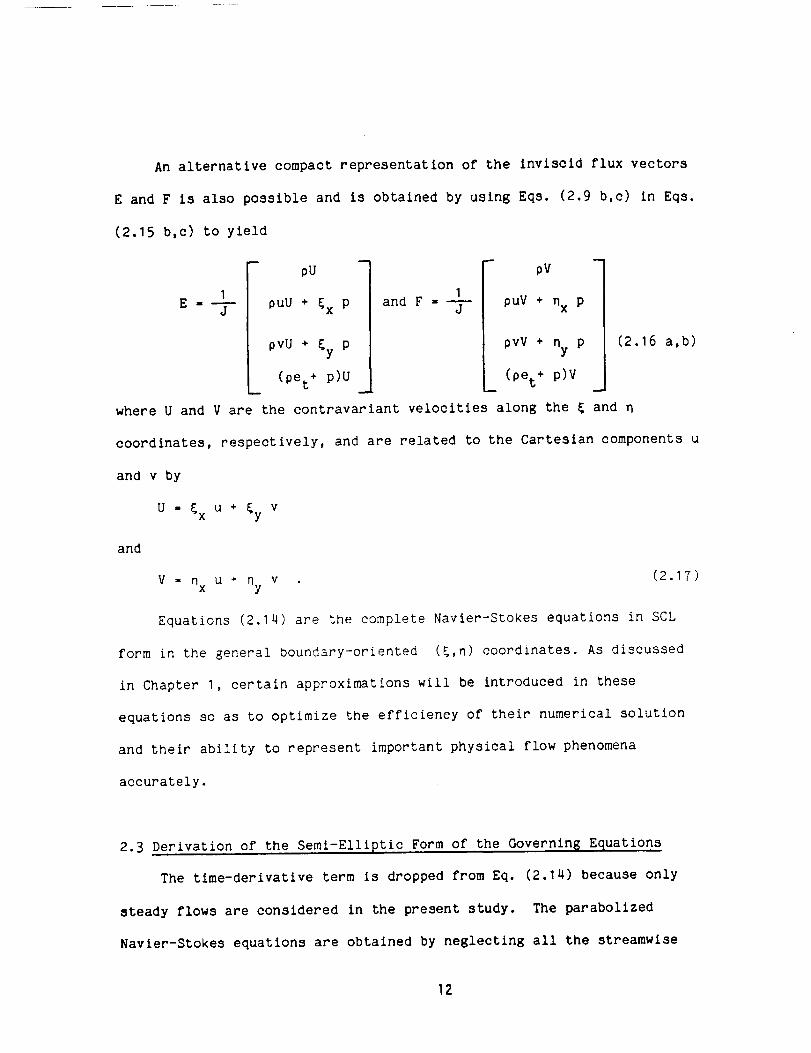
An alternative compact representation of the Invlscid flux vectors
E and F is also possible and is obtained by using Eqs. (2.9 b,c) in Eqs.
(2.15 b,c) to yield
m
IE _ m
J
pU
puU + _x p
pvU + _y p
(Pet+ p)U
Iand F -
J
pV
puV + nx p
pvV + ny P
(Pet+ p)V
(2.16 a,b)
where U and V are the contravariant velocities along the _ and q
coordinates, respectively, and are related to the Cartesian components u
and v by
U - _x u ÷ _y v
and
V _ nx u + ny v (2.17)
Equations (2.14) are the complete Navier-Stokes equations in SCL
form in the general boundary-oriented (_,n) coordinates. As discussed
in Chapter I, certain approximations will be introduced in these
equations so as to optimize the efficiency of their numerical solution
and their ability to represent important physical flow phenomena
accurately.
2.3 Derivation of the Semi-Elliptic Form of the Governin$ Equations
The time-derivative term is dropped from Eq. (2.14) because only
steady flows are considered in the present study. The parabollzed
Navier-Stokes equations are obtained by neglecting all the streamwise
]2

diffusion terms• This involves dropping the second-order derivatives
( 22 /_2 ) and the cross derivatives ( 22 /_ _n ) in the viscous
terms. This approximation is supported by the fact that the streamwise
diffusion is negligible compared to the normal diffusion in most of the
regions of the flows under consideration. This approximation is
appropriate only if the (_,_) coordinate system is a body-orlented,
near-orthogonal coordinate system, that is, the _ coordinate is nearly
aligned with the streamwise direction and the n coordinate is nearly
orthogonal to it. The reduced set of equations can be written as
follows.
_E _F
m + m = __ (Fv) (2.18)
where E, F and F are as given in Eq. (2 15)V • •
It should be emphasized that the above set of equations is
'parabolized' and not parabolic. The mathematical character of the
system of equations (2.18) depends on the manner in which the streamwise
pressure gradient term p_ is treated. If p_ is prescribed, as in the
case of classical boundary-layer theory, the system is parabolic. In
this case, a marching method can be employed to obtain the solution for
this system. This method of solution is very efficient, but it does not
have any mechanism for including upstream influence and is, therefore,
not suitable for flows with separation and sudden streamwlse changes in
boundary conditions. When the p_ term is treated as unknown and forward
13

differenced, the system of equations is no longer parabolic but has an
elliptic character.
When the parabollzed Navler-Stokes equations are solved as an
Inltal-value problem, as in the case of slngle-sweep marching solutions,
the ill-posedness of the equations leads to 'departure solutions'
similar to the elgensolutions of the viscous sublayer equations proposed
by Lighthill [23]. Vigneron, Rakich and Tannehill [24] have described a
method for suppressing the departure solutions in their study of
supersonic flow over delta-wings. They introduced a parameter, m, to
split the pressure gradient term Px into 'm Px '' which was backward
differenced and treated implicitly, and (1-m)px. The latter term, even
when represented using a backward difference, led to instabilities and,
hence, was dropped entirely. This is appropriate if the flow is
predominantly supersonic, as in the case these authors considered, but
not in general. These authors performed a characteristics analysis for
the inviscid as well as the viscous limits of the equations. From the
viscous analysis, they found that the equations are well posed for space
marching when
y M 2x
I+(Y-I ) M 2x
and _- I if f(M x) > I
- f(M x) if f(M x) _ I (2.19 a)
, (2.19 b)
where M - _ . (2.19 c)x a
In the present study, the pressure-gradlent term is split in the
manner described above, but Is dlscretlzed so as to include upstream
]4
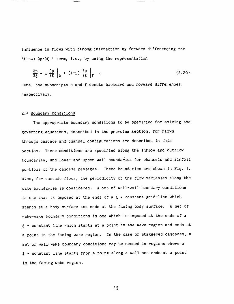
influence in flows with strong interaction by forward differencing the
'(l-m) _pl_ ' term, i.e., by using the representation
_)P m + (l-m) (2 20)f "
Here, the subscripts b and f denote backward and forward differences,
re spect ively.
2.4 Boundary Conditions
The appropriate boundary conditions to be specified for solving the
governing equations, described in the prevoius section, for flows
through cascade and channel configurations are described in this
section. These conditions are specified along the inflow and outflow
boundaries, and lower and upper wall boundaries for channels and airfoil
portions of the cascade passages. These boundaries are shown in Fig. I.
Also, for cascade flows, the periodicity of the flow variables along the
wake boundaries is considered. A set of wall-wall boundary conditions
is one that is imposed at the ends of a _ = constant grid-line which
starts at a body surface and ends at the facing body surface. A set of
wake-wake boundary conditions is one which is imposed at the ends of a
- constant line which starts at a point in the wake region and ends at
a point in the facing wake region. In the case of staggered cascades, a
set of wall-wake boundary conditions may be needed in regions where a
- constant line starts from a point along a wall and ends at a point
in the facing wake region.
15
2.4.1 Inflow and Outflow Boundary Conditions
For the problems considered in the present study, the flow near the
inflow and outflow boundaries behaves in an almost inviscid manner.
yon Mises [25] has carried out a characteristics analysis for inviscid
systems and found that for subsonic flows, all the characteristics are
real, with two of them being positive and one negative. Using the
counting principle of Courant and Hilbert [26] that one boundary
condition is to be specified per entering characteristic, this requires
that two conditions are to be specified at the inflow boundary, and one
at the outflow boundary.
In Ref. [27], McDonald and Briley have described a specific set of
boundary conditions. They considered a typical duct flow proceeding
from a large reservoir and exhausting into a plenum. The reservoir
conditions and the plenum static pressure were known. This duct flow
model leads to prescribing the reservoir total conditions and the plenum
static pressure. The specified stagnation temperature and pressure
constitute the two required inflow boundary conditions and the specified
static pressure constitutes the one outflow boundary condition.
In the present study, at the inflow boundary, the total pressure
prescribed for cascade flows is that corresponding to a uniform velocity
profile, while the stagnation temperature is taken to be constant. For
channel flows, the conditions prescribed at the inflow boundary are the
velocity and static temperature profiles corresponding to a fully
developed flow in the channel.
16

In the problems considered, the outflow boundary is situated far
downstream of the cascade of airfoils or the channel constriction, so
that uniform static pressure Is an appropriate condition.
As the static pressure at the inlet is not specified, the mass flow
in the configuration is not set a priori and pressure waves can escape
upstream, avoiding the problem of reflecting waves discussed by Rudy and
Strlkwerda [28]. To facilitate a marching procedure, the conditions at
the inflow boundary are obtained by assuming the velocity-profile shape,
guessing a representative magnitude characterizing this profile, and
obtaining the static pressure using the prescribed total pressure. The
guessed representative velocity magnitude, Uavg , is then updated as the
overall solution evolves. For channel flows, McDonald and Briley [27]
have suggested updating the total pressure distribution within the
boundary layer, in order to maintain the required velocity- and
temperature-profile shapes prescribed at the inflow boundary. This
implies that for fully developed flow conditions at the inlet, as used
in the present channel-flow studies, the total pressure distribution has
to be updated over t_e entire channel width.
The procedure for updating the velocity profile for cascade flows
will be described in the next chapter.
2.4.2 Wall-Wall Boundary Conditions
The governing equations given by Eq. (2.18) consist of one first-
order equation, namely, the continuity equation, and three second-order
equations, namely, the x- and y-momentum and the energy equations.
17

Here, the order refers to the highest-order derivative in the n
direction. These comprise a system of seventh order with respect to n,
so that a total of seven boundary conditions need to be specified along
the two n - constant boundaries. At the wall, the no-sllp boundary
condition is imposed; also, the walls are assumed to be impermeable and,
hence, there is no injection or suction at the surface. In addition,
the temperature, T w , at the surface is specified. These constitute a
total of six boundary conditions at the two surfaces. Therefore, one
additional condition has yet to be specified. A valid flow approxima-
tion such as (_P/_n) = 0 can be imposed as an additional boundary
condition. The resulting solution will reflect the approximations
inherent in the boundary condition. Another method to obtain the
additional condition is to write the governing equations in one-sided
difference form at the wall, as has been done by Rubin and Lin [29] anc
Briley and McDonald [30].
In the present study, an approximate form of the normal momentum
equation, obtained by dropping the viscous terms in that equation and
written at the first cell center near the wall surface, is used as the
additional condition. The viscous terms in the normal momentum equation
can be shown to be negligible near the wall surface for most of the
flows considered in this research.
In order to ascertain that enough independent equations are
available at a particular streamwlse location, a typical grid llne along
the n direction, consisting of five computational points as shown in
Fig. 2a, is considered. Counting four unknowns, namely,
18
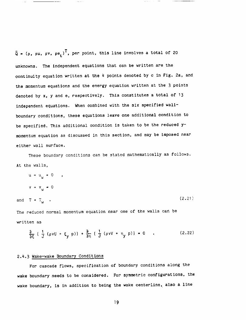
- (p, pu, pv, Pet)T, per point, this line involves a total of 20
unknowns. The Independent equations that can be written are the
continuity equation written at the 4 points denoted by c in Fig. 2a, and
the momentum equations and the energy equation written at the 3 points
denoted by x, y and e, respectively. This constitutes a total of 13
independent equations. When combined with the six specified wall-
boundary conditions, these equations leave one additional condition to
be specified. This additional condition is taken to be the reduced y-
momentum equation as discussed in this section, and may be imposed near
either wall surface.
These boundary conditions can be stated mathematically as follows.
_t She walls,
U = U = 0 ,W
V = V = 0W
and T = T . (2.21)w
The reduced normal momentum equation near one of the walls can be
written as
2-[ 5 (pvU + &y p)} + _ { I_--_ _ (pvV + ny P)} " 0 . (2.22)
2.4.3 Wake-wake Boundary Conditions
For cascade flows, specification of boundary conditions along the
wake boundary needs to be considered. For symmetric configurations, the
wake boundary, is in addition to being the wake centerline, also a line
19

of symmetry. For unstaggered cascades, a 'line-periodic' grid is
employed. In this type of grid, the same n-coordinate line connects the
corresponding periodic points, such as points I and 5 or 0 and 4 in
Fig. 2b. In this case, the periodic-boundary conditions can be enforced
implicitly. The periodicity condition is that the corresponding values
of all the flow variables, Q (p pu pv, Pet)T" , , , and the normal
derivatives, u , vn and Tq, of the velocities and temperature which are
governed by second-order equations, namely, the momentum and energy
equations, must be the same at corresponding periodic points alone the
wake boundaries. It should be mentioned that, in terms of the conserved
variables, Q (p, 0u, pv, Pet)T- , the repeating condition on the n-
derivatives must be satisfied for all four elements of Qq. This
condition can be written as
- or (2.23)
for a typical computational llne consisting of points I through 5 as
shown in Fig. 2b. Imposing the periodicity boundary condition described
above between points I and 5, leaves a total of 16 unknowns counting
four unknown variables per computational point. The system of equations
that can be written along this computational line consists of the
continuity equation at 5 points, and the momentum and energy equations
at 4 points, denoted by c, x, y and e, respectively, in Fig. 2b. As
periodicity has already been imposed, the continuity equation, which is
of the first order, Written employing points 4 and 5, becomes identical
2O
to that employing points 0 and I. Hence, there are only 16 independent
equations and the system is closed. Also, in the case where symmetry
exists along the wake boundary, the viscous terms in the y-momentum
equation can be dropped, and this reduced first-order equation can be
written employing points I and 2.
2.4.4 Wall-Wake Boundary Conditions
This type of boundary condition is needed for cascades with stagger
when a 'region-periodic' grid is employed. A 'region-periodic' grid is
one in which the corresponding periodic points in the flow are not
connected by the same n-coordinate line. This type of grid has to be
employed for cascades with large stagger in order to avoid excessive
skewness of the coordinates. The use of this type of coordinates, in
conjunction with a marching procedure, forces the p_riodicity condition
to be imposed in an explicit manner.
Figure 2c shows a typical grid consisting of six points along an n-
coordinate line in the wall-wake region. The 18 independent equations
along this line consist of the continuity equation written at 5 points
and the momentum and energy equations written at 4 points, in addition
to the reduced momentum equation written at the wall surface. The six
boundary conditions consist of the zero slip, zero injection/suction and
the specified temperature at the wall surface and the specified velocity
and temperature conditions at the wake boundary. The conditions at the
wake boundary are obtained from the corresponding periodic point along
2]

the upper wake boundary in the flow. These conditions can be stated
mathematically as follows.
At the wall, the conditions are
u- u - 0 ,W
V- V - 0W
and T - T . (2.24)W
Along the wake, for example, at point 0 in Fig. 2c, the conditions are
U 0 " U a
V 0 _ V a
and T o - Ta . (2.25)
Here, '0' and 'a' are the corresponding periodic points.
2.4.5 Wake-wake Boundary Conditions (Region-Periodic Grid)
Along this type of boundary for staggered cascades employing a
region-periodic grid, the periodicity condition is imposed in an
explicit manner. The independent equations to be considered along a
typical computational line consisting of six grid points 0 through 5 are
the continuity equation written at 5 points and the (x,y) momentum and
energy equations written at 4 points. The boundary conditions consist
of the specified values of Q - (p, pu, pv, Pet )T at point 5, obtained
from the values at the corresponding periodic point in the flow, such as
point b in Fig. 2d. For this purpose, the most recent values of Q are
used. This implies that only three more boundary conditions can be
22
supplied for the seventh-order system. Hence, the velocities u and v
and the temperature, which are lagged in time, are specified at point O.
These conditions can be stated as follows.
Along the wake, at point 5,
Ps - Pb ' u5 - ub , vs - vb and T5 - Tb
and at point O,
u0 - ua , v o - va and To - Ta .
(2.26)
(2.27)
23
CHAPTER 3
NUMERICAL PROCEDURE
The interacting parabolized Navier-Stokes equations (2.18),
described in the preceding chapter, are a set of nonlinear coupled
partial differential equations. Analytical solution of this system of
equations exists only for a small, special class of problems. Hence,
for the general problems of present interest, a numerical solution of
these equations is scught.
The linearizaticn and discretization of the governing equations,
the solution procedure for the discretized set of equations, the
implementation of tee boundary conditions, including the periodicity
boundary condition f:r cascade flows, as well as the treatment of
problems with flow separation are detailed in the following sections of
this chapter.
3.1 Quasi-lineariza_i}n and Discretization
The system of g=verning equations (2.18) is first re-wrltten here
for easy reference.
aE + a_[. L (F) (3.1)aF_ an an ,
where
_x _yE - 3-- _ + 3-- _ ,
nx nyand F - _-- E + ]-- F . (3.2)
24

FO* ,ur,,_,r,,,.,_
As mentioned above, this system of equations is nonlinear.
Therefore, these equations must be linearized or quasi-linearized in
order to obtain a system of algebraic equations amenable to numerical
solution. In the present study, employing forward marching for the
solution vector Q, a quasi-linearlzation of the nonlinear terms at a
given streamwise station is carried out about the solution at the
preceding streamwise location. From Eq. (3.2), it is seen that the
quasi-linearization of the inviscid flux vectors E and F requires that
the flux vectors E and F be quasi-linearized. This is achieved by using
Taylor'8 series expansions. The results can be expressed as follows.
_i+! . _i + _i Ai_ , (3.3
_i+I . _i + _i Ei 5 , (3.2
where
. 6i+I_ 6i
_i . @_i and _i = 8-2i • (3.5 a-c
Here, the superscripts i and (i+I) denote two successive streamwise
locations as shown in Fig. 3. The quantities with superscript (i+I) are
the unknown terms, which contribute to the nonlinearities in the
equations.
Recognizing the fact that the Inviscid flux vectors, E (Q) and
F (Q) are homogeneous functions of degree I in Q, and using the property
of homogeneous functions (see Ref. [31]), one can write
25
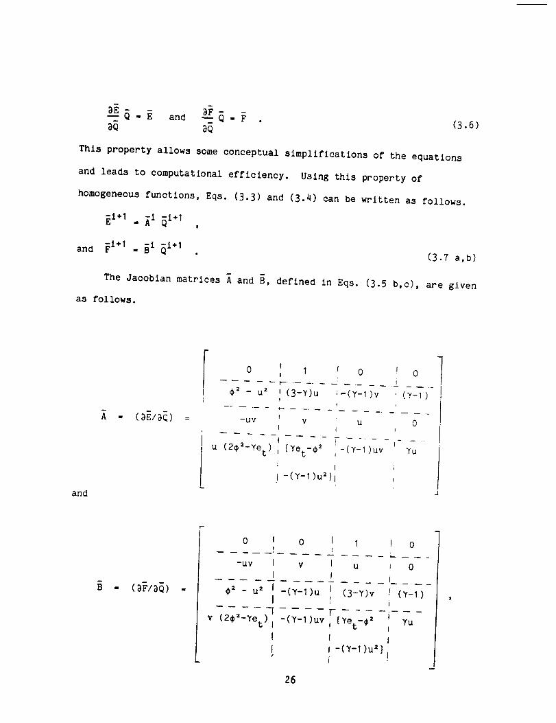
B___ . _ and B-_FQ I F . (3.6)
This property allows some conceptual simplifications of the equations
and leads to computational efficiency. Using this property of
homogeneous functions, Eqs. (3.3) and (3.4) can be written as follows.
(3.7 a,b)
The Jacoblan matrices A and B, defined in Eqs. (3.5 b,c), are given
as follows.
and
(Y-_)
0 i I I 0I
I"
¢2 _ Ua I (3-Y)U ;-(Y-I)vI
t
I--UV V U
I
= (_E/_Q) = 0
iu (2¢_-Yet) , [Yet-¢ 2 -(Y-1)uv
I -(Y-1 )u2}
i
Yu
0 I 0
-uv I v
I
I
u 0
_2 _ u 2 1 -(7-I)u (3-7)v (_-I)I
v (2_a-Yet)i TI -(Y-I)uv i {Yet-Oa Yu
I
I 0-(Y-I)u'} l' i
26

where CZ _ (Y-I) (u=+ v= ) (3.8 a-c)2 _
as
[32].
i+IE
with
Using Eqs. (3.7) and (3.2), the flux vectors E and F can be written
El+l . i+1
E
where _l (_)i+1 _i + (_)i+1 _l . (3.9 a,b)
Similarly,
Fi+1 . _i _i+I
h glwhere _i = (j)i+1 _i + . (3.9 c,d)
As the metric terms at (i÷I) station are known quantities, the
metric terms involved in Eqs. (3.9 a-d) are evaluated at station (i+I).
This type of quasi-linearization has been employed by Schiff and Steger
It is different from that employed by Steger [7], who used
= E i + A i AiQ (3.10 a_
A i = a--_Ei . (3.10 b)
at
iThe Jacobian matrix A contains metric quantities evaluated at station
i. The _~ on the Jacobian matrices A and B in Eq. (3.9) is used to
denote that the metrics in these matrices are evaluated at station
(i+I), and distinguishes these matrices from the Jacobian matrix in
Eq. (3.10).
27

The viscous term Fv is quasi-llnearlzed as follows. A typical term
of Fv is of the form (_ _ . Starting with the Taylor's series
_8)i+Iexpansion for (_ _ and re-arranglng leads to the expression
_8)i+I i+I (_8)i i+I
Further, it is observed that the term 8 is homogeneous of degree zero,
in Q. Hence,
(aS/_Q) Q = O. (3.11 b)
Therefore, Eq. (3.11 a) becomes
_8)i+I i+I 88 i i+I )i _i+I(a _-_ = _ (-_n) + _ (_8/_Q (3.11 c)
Using Eq. (3.11 c) the viscous term F i+I can be written as' V
Fi+1 = rZi ÷ _i _i÷IV V V
where a typical term of _iv is of the form i+I (___)a8i , and of _i _i÷I isV
i+I i :i+I(_8/_Q) . Again, the ~ denotes that the metrics involved
are evaluated at station (i÷I).
The discretization of the derivative terms is discussed next. The
i+I
term [__m)_ is considered first. This term can be_-derivativea£
written as
_E I+I _E i+I f_E]i('_) - e, (_) + (l-e,) ,-_, .
(3.12)
28

The values of 61 are chosen depending on whether an implicit, explicit
or the Crank-Nicolson scheme is to be employed. The various values of
8_ commonly employed, and the corresponding schemes, are
01
I I
= 0
I12
for an implicit scheme ,
for an explicit scheme ,
for Crank-Nlcolson scheme (3.13)
Also, depending on the type of differencing and the desired
accuracy, one can write
(_E] I+I Ai E_, - (1+e_) _
I-IA E
e.2 A_(3.14)
where A i is the forward difference operator defined by Eq. (3.5 a).
The type of differencing, and the corresponding order of accuracy, for
various values of 02 are given as
02
I -I/2,
0 ,
I/2 ,
central, O(A_ 2)
two-point backward, O(A_)
three-point backward, O(A_ 2) (3.15)
Combining Eqs. (3.12) and (3.14) leads to,
+ (1-e_) DE i i A i-I E. (i+e2) A E e . (3.16)A_ 2 A_
An explicit scheme usually has some stability condition such as the
Courant-Frledrichs-Lewy (CFL) condition associated wlth it. Hence, an
implicit scheme, corresponding to e_ - I, is employed in the present
t
work, to enhance the numerical stability of the resulting method. To
facilitate a marching type of procedure, either two-polnt backward
29
differencing or three-point backward differencing has to be employed.
In the present work, the two-point backward differencing, with 82 - O,
has been employed.
for (_) from the governing differentialSubstituting equation
(3.1) into Eq. (3.16) gives
a )i+1 aEi A i E A i-I E
= (I+82) A_ 82 At "
(3.17 a)
Equation (3.17 a) can be rearranged as follows:
A i E 8_ Ai-1 - _ A_ a i+1= 1+ez E 1+e, _ (F-Fv)
a i- _ At -_ (F-F v) (3.17 b)1+82
Substituting for the quantities at station (i+I) using the quasi-
linearization given by Eqs. (3.9) and (3.11), Eq. (3.17 b) can be
rewritten as
Ei _i+I _ E i . 82 At-1E - e--_L- A& a {(_i _ _ i) _i+I _ _ i}1+8= 1+e= T6 -v v
- A6 1-81 a_ (F_Fv)i (3.18)1+e= an
Equation (3.18) can be re-arranged to contain the unknowns at station
(i+I) in the incremental or delta form, by subtracting
+ e_.L. L {(At_§i)1+8= an v
from both sides of Eq. (3.18) and is given as
3O
Here,
l+e= _n
. El _ _i _i _ _i-_+ 1+82 E - A_ 1+e2
1+e= an v v(3.19 a)
Ox
and B i _i = O. (3.19 b-d)v
It may be important to recall that Eqs. (3.19 b,c) are obtained
from the definitions of the Jacobian matrices A and B, given by Eqs.
(3.9 b,d), and by using the homogeneous property [Eqs. (3.6)] of the
flux vectors E and F.
For an implicit scheme employing a two-point backward difference,
e_ -I and 82 " O. Hence, Eq. (3.19 a) reduces to the following.
• a i -i_i _ + _ {(B _Bv) _i_}
a _i F i ) (3.20). E i _ _i _i - A_ _-_ (B i - v
The next step in the numerical procedure is the introduction of
upstream influence. For flows with strong viscous-lnviscid interaction,
as mentioned in Section 2.3, the streamwise pressure gradient term is
split according to Eq. (2.20) and upstream influence is introduced by
31

forward differencing the '(l-u) ap/a_ , term.
the governing equation (3.1) can be written as
where
_pDE + aF a (Fv) - - a --a_ an an a_f
aI
u u
J
0
(I-.,) _x,f
(I-,,,)Ey,f
0
With this 'm - split',
(3.21 a)
(3.21 b)
The subscript f on the pressure gradient term denotes that this
term is forward differenced and those on the metrics _x and _y denote
that these are obtained using coordinate values at station (i+2). This
representation of the metric terms was arrived at by applying the
procedure for a test case in which a fully developed flow was reproduced
in a straight channel using a coordinate system with metrics varying
along the streamwlse direction.
The flux vector E is different from E given in Eq. (2.16), in that
the pressure terms in it are multiplied by the factor m. It is given as
pU
* I
E - "7- puU + _x up
pvU + _y up
(Pet+P) U (3.22)
where U is the contravariant velocity given by Eq. (2.17 a).
32
For low subsonic flows considered in the present study, according
to Eq. (2.19), m - O. This implies that the total streamwise pressure-
gradient term is forward differenced. Also, it is clear from
Eq. (3.21 a) that the streamwise pressure gradient term is no longer in
the SCL form. This necessitates that the pressure gradient term pn
should no longer be in the SCL form, as the starting governing equations
were written in the conservation form in Cartesian coordinates.
Accordingly, Eq. (3.21 a) must be written in the following form.
_E _F _P _ (Fv) - - a _p (3.23 a)÷_ ÷ b _-_-_-_ _f
where
Ib -
J
0
(I-_) nx
and F _ F - b p
i (l-m) ny
o-t
(3.23 b)
. (3.23 c)
The procedure for quasi-linearization of Eq. (3.23 a) is similar to
that used to obtain Eq. (3.20). The resulting equation has an extra
source term on the right hand side, arising out of the pressure gradient
(_p/_)f term. The quasi-linearized form of Eq. (3.23 a) becomes
. E*i_ _*i_i
i+I AI+I- a p . (3.24)
33
The asterisk on the Jacoblan matrices A and B denotes that these are
obtained from the corresponding flux vectors E and F , respectively.
A possible method of solution of Eq. (3.24) Is to employ an
alternatlng-dlrection explicit (ADE) method. In the first step of this
method, AIQ is computed starting at the inflow boundary and proceeding
towards the outflow boundary and in the second step, Ai+Ip is computed
starting from the outflow boundary and proceeding towards the inflow
boundary. Such a method requires the inclusion of a tlme-derivatlve
term, Pt' in the momentum equations containing (Sp/S_)f term, in order
to unlock the solution from its initial conditions. This method, llke
the pressure updating procedure used previously by K. Ghia and U. Ghia
[33], is capable of transmitting the downstream disturbances upstream
efficiently. It is, however, algebraically much simpler and has been
successfully used by Barnett and Davis [34], for solving supersonic
external flow problems.
With the inclusion of the time-derivative term, the governing
equation (3.23 a) assumes the following form.
_-_ + _ + b - _ (Fv) = - a _f + a(3.25)
The quasillnearized form of Eq. (3.25) is obtained by utilizing Eq.
(3.24), in addition to dlscretizlng the (_p/_t) term as
1+1
(_t) " A'-'_-I (pl+l,n*l/2 - Pl+l,'n) (3.26)
34
I+I,n+I/2 i,n+1/2and quasilinearizing p about p . The resulting
equation is
_*i Ai_ + A_ [ __ {(_*i _ _) Ai_} + bi+1 --_ {(_p)i__ Ai_}_n _Q
I+I
a {(_p)i Ai_ }]At
_Q
*i _*i _i _ (_*i _i bi+1 _pi _ (_i)}- E - - a_ {T_ ) + _n - T_ v
+ ai+1 A_ i,n+1/2 i+1,n) I{___ (p _ P _ Ai+ pn} (3.27)
The diseretization of the above equation in the n direction is
considered next. The discretization is performed such that the
discretized form of the inviscid portion of the equations constitute a
consistent set of equations by themselves; the viscous portion of the
equation is also discretized in a self-consistent manner. The inviscid
part of Eq. (3.27) is given by
-*i _ A i " I 3 (_p)i
8Q
i+l
a {(___p)i Ai_}]at
_Q
+ ai+1 {_._(pA_ i,n+1/2 - pi+1'n) _ AI+I p} (3.28)
All normal derivatives are represented by central differences, with
the first-order derivative representation involving points across one
normal mesh interval only. The discretized equations are second-order
35

accurate in the n direction. Equation (3.28) is written at a normal
mesh midpoint, J+I/2 , as
I -*i A_{(_*i al_ )j + (A AI_ )j+1 } + _ [( _*i AI_ )J+1 - (_*i AI_)j
+ b) +l { --(aPI _ (ap i AI_)j}]+I/2 AiQ)j+l -aQ aQ
A{ a]+l {(aPi AIQ )J+l + (apl Ai_2 At +I/2 aQ BQ
)j}
I *i *i • _i)j- _ {Ej + Ej+I _ ( _'i _ ( _*i _i)j+1 }
An )j+1 - (B )j j+I/2 I }
1 a]+l [ A_ i,n+1/2 l+l,n)j++ "2 +I/2 _ {(p - p I
)j _ Ai+1 n] (3 29 a)+ (pi,n+I/2 _ pi+1,n } - Ai+1 P;+I PJ "
where
i+l I i+I i+I
aj+i/2 = _ (aj * aj+ I)
and
b]:1 1 ,bi+1 i+II/2 = 3 _ j + bj+1) (3.29 b,c)
In order to include the viscous terms at mesh point j, the inviscid
part of the equation should also be written at J. This is obtained by
writing a discretlzed equation similar to Eq. (3.29) at location (J-I/2)
and forming the arithmetic mean of this equation and Eq. (3.29). The
resulting equation is
36

A_4- -"--"--
2 An
r i+I
- _ Laj ÷I/2
I *i---_ { Ej÷I
- (B )j-1-*i i)j
2 An
i +1 (pij+I+ bj,1/2
1 i'1 _._._{(pi,n*l/2 _ pi*l'n)j, 1
* --_ a j+l/2 At
i,n+I12
+ -_ aj_i/2 At
1 r i +1- _" [aj+I/2
_.i.I {(_p.iAi_ )J*_ _Q
+ bJ ÷I/2 BQ
+ bj_i/2 BQ @Q
@Q
i+I {(_2i AiQ)J + (_i Ai_)j_I} ]
+ aj-1 12 _ _Q
)j+1 + eJ-I -(A. _i)j_1 } + ._ {Ej .(_*i )j}
(p_,O i,_- Pj_l_
1+1+ (pi,n*I/2 _ p ,n)j
i*1,n) + (pi'n+I/2 - pi+1'n)J -I}- p j
+ Ai+1 n )]i+I (Ai+I p_ Pj-I
(Ai+1 n + Ai+1 n) + aj_i/2PJ*I PJ
(3.30)
37

The dlscretlzatlon of the viscous terms in Eq. (3.27), for example,
_(B_ AIQ)/_n , is considered next. The viscous flux vector Fv and the
Jacobian matrix Bv:
can be given as follows:
F =v J Re
0
_l U + _3 Vn n
L s U + _'2 Vn n
t_ uu ÷ _, vv ÷ _, (uv)n n n
U 2 + V 2
÷ _ (et 2 )n (3.31 a)
v J Re
where
0
- Z_ (_)n
- _'3 (v)P q
- Za (_v)p n
.......... l .... " ....
0 I 0 _0
........... i ........ I .....
_,2 (-_) n 0
t, (_u)p n
, v) (1)+(_-_ ) (_ n _'_ n
= et - (u2+v2),
4 + nYzL s = _ _X2
38

4 2
£2 " nx 2 + _ _y
and
£, = (nx ny)13
Y ( 2 + ny2) . (3.31 b-g)£_ s p--{ nx
It should be mentioned that when the term (BV
AQ) is formed, the AQ term
should be contained in the n-derivatlves appearing in Eq. (3.31 b). A
_(B 5)_n
]. Fortypical term of this product can be expressed as [a
example, for the element corresponding to the (2,2) location of
The discretlzation of a(B 6Q), a = Z_ , 8 = --I and 6 = A(_v).v p
typical term _-_ {_ _n (8 6)} is performed by evaluating the quantity
in brackets at two successive mesh mid-points, such as (j+I/2) and
(j-I/2), and forming a difference expression at the mesh point j to
obtain a second-order accurate representation for this term. This is
outlined below.
_n
where
}j = A--n _ (8 6))j+i/2 _ (8 6))j_i/2
I { (Sj - 8j 6 )}(a _-_ (8 6))j÷i/2 " A-_ aj÷I/2 +I 6j+I j
I (Bj 6j - 8j )}(a _-_ (8 6))j_i/2 " A--_{aJ-I/2 -I 6J-I "
and
(3.32 a-c)
39
Using the discretization described by Eqs. (3.30) and (3.32), Eq.
(3.27) can be written in a compact form as
Aj AIQj_I + Bj AIQj + Cj AIQj+I = Dj .
The discretlzatlon described above applies at a general interior
point; the treatment of boundary points will be discussed in the next
section.
Equation (3.33), written at all the mesh locations J along a line
(i+I), results In a block-trldlagonal system of equations, with Aj, Bj
and Cj being (4x4) matrices. This system of equations, can then be
solved using L-U decomposition of the coefficient matrix of the system.
The implicit solution procedure for such a system can be found in
Ref. [35], by Anderson, Tannehill and Pletcher.
(3.33)
3.2 Details of the Solution Procedure
The solution procedure consists of two time steps. In the first
step, the solution proceeds from the inflow boundary towards the outflow
boundary, employing Eq. (3.25) to update Q . The pressure field is
updated in the second step of the procedure. This step proceeds from
the outflow boundary towards the inflow boundary. The outflow boundary
condition on pressure is directly employed during this step. These two
steps can be expressed as follows.
Rn+I/2 (_p]n + a f_p]n+I/2Step I: - - a "B_'f "@t' (3.34 a)
40

Step 2: Rn+I/2 - - a (_p]n+la_jf+ a r_p]n+1,atJ (3.34 b)
where R contains all terms in Eq. (3.25) except the pressure terms which
appear explicitly in the above equation. In Eq. (3.34), superscripts
denote time levels. Thus, for example, the superscript (n+I/2) denotes
that the time derivative is evaluated at time level (n+I/2). Backward-
difference approximations are used for the time derivatives, so that the
time derivative at (n+I/2) employs the pressure at time levels n and
(n+I/2).
A simpler equation for the second step can be obtained by
eliminating Rn+I/2 between equations (3.34 a) and (3.34 b). The
resulting equation is
_atjr_p]n+I/2 r_ap)_+1 + _atjf_p]n+1- {a_)f + = - _a_ (3.35)
The discretized form of Eq. (3.35) at station (i+1) is
(pi+2,n i+I A_ i+I,n+I/2 i+I n_ _ P ,n) + __ (p _ P , )At
(pi+2,n+1 i+1,n+1 A_ i+1,n+1 i+I,n+I/2). _ - p ) + m (p - p (3.36)At
i+1,n+1From this equation, p can be solved for in an explicit manner as
i+I ,n+1 i+I )n i+2,n i+2,n+1P = [P -p + p
+ A_ (2pi+1,n+1/2 i+1,n) A_A'E" - P ] / {I+_'E) (3.3?)
Equation (3.37) is applied along lines of constant n and the
pressure field is updated by marching upstream. The prescribed
condition on the pressure at the outflow boundary is imposed via the
41

i+2,n+1p term in Eq. (3.37). The two steps described above constitute
one global iteration, during which the flow solution is advanced from
the time level n to time level (n+1).
If the pressure terms are retained in the SCL form, then the
equation for the upstream marching step, corresponding to Eq. (3.35),
will be a set of two equations in the single variable p. This system
can be reduced to an equation similar to Eq. (3.35) by combining the two
equations after multiplying each of them by the appropriate metrics.
This is equivalent to taking a projection of the two equations along a
llne of constant _.
3.3 Updating of Velocity Profile at the Inflow Boundary
The reference velocity, U , characterizing the velocity _rofileavg
at the inlet, needs to be updated before the next global iteration is
performed. This is necessary because at the inflow boundary the total
pressure and temperature are prescribed as boundary conditions, so that
U has to be guessed to initiate the solution procedure. The updatingavg
of U is as follows. At the inflow boundary, knowing the dimensionalavg
total pressure PO and the dimensional static pressure p (which is
evaluated through the upstream marching step), the local Mach number M
can be obtained using the isentropic relation
POm m
P
Y21 M2)7/_-I(I+ --=. (3.38 a)
42

Then, using the dimensional total temperature T O prescribed at the
inflow boundary, the static temperature T can be obtained from the
following relation
TO"V - (1+ M')T
(3.38 b)
The dimensional density p can then be found, using the equation of
state, as
p - p /R T . {3.38 c)
Knowing M = and T , together with the definition of the local sonic
velocity, the local dimensional speed V (- {u .2 + v'2}I/2), can be
determined from the relation
V 2 = M 2 ¥RT (3.38 d)
The Cartesian components of the velocity u and v can be
determined from the given flow direction, e, at the inlet so that
u = {V 2 /(1+tanZ8)} I/2 (3.38 e)
and
v - u tan8 (3.38 f)
The reference velocity U is then obtained using Eq. (2.6) andavg
all the variables are then re-nondlmensionallzed.
43

3.4 Convergence Criteria
The two steps of the solution procedure described in Section 3.2
are repeated until convergence is achieved. To test for convergence,
the maximum absolute value of the error (L®-norm) and the root-mean
square of the relative error (L2-norm) in the pressure field are
monitored. These are defined, respectively, as
max I I.1.IIMAxp] p]nCabs J-1 ,JMAX
and
i,n
JMAX IMAX Pj )2 }1121ere I - { [ [ (I---i,n+1 (At IMAX JMAX)
j-1 i.I p_J
(3.39 a,b)
< I0-4Convergence is said to have been achieved when Cab s . and
E < 10-6rel
3.5 Implementation of the Boundary Conditions along n = Constant
Boundaries
In the present study, the boundary conditions at the walls and, in
the case of cascade flows, along the wake boundaries are implemented in
an implicit manner, consistent with the numerical procedure employed in
the interior of the computational domain. The implicit treatment of
these boundary conditions in an otherwise already implicit solution
procedure removes the mesh spacing constraints encountered in an
explicit scheme and also aids in enhancing the convergence process.
44

U " UW
3.5.1 Wall Boundary Condition
As mentioned in Section 2.4.2, the zero-slip and zero suction/
injection conditions at the wall, together with the wall temperature,
are specified. These are written as
- O,
V = v = 0w
and T = Tw
Expressed in terms of the increments in the variable
= (p, pu, pv, Pet)T, Eq. (3.40) yields
i+I " Ai i A i- u Alp + (pu) = p u ,
i+I " A i i A i- v Alp + (pv) = p v
(3.40 a-c)
i+I " i i iand - e t Alp + A (pe t ) = p A e t (3.41 a-c)
In the above equation, all quantities with superscript (i+I) are
known from the conditions given by Eq. (3.40) and the right-hand side of
Eq. (3.41) can be evaluated using the known solution vector _i at
station i. The three equations given by Eq. (3.41), together with
either the continuity equation or the reduced y-momentum equation,
constitute the four equations at the wall boundaries.
3.5.2 Periodicity Boundary Condition for Cascades
For flows through cascades employing a 'llne-perlodlc' grid, the
periodicity boundary condition can be imposed in an implicit manner.
The periodicity condition, as described in Section 2.4.3, requires that
45

the flow variables have the same values at corresponding periodic points
along the wake boundaries. When this condition is imposed, the
discretized equation (3.33) assumes the following form.
At J-l,
A I AiQJMAX_I + B I AIQI + C I AiQ2-D I
and, at J-JMAX-I,
AjMAX- I AIQJMAX-2 + BjMAX_ I AIQJMAX-I ÷ CjMAX_ I AIQI - DjMAX_ I
(3.42)
(3.43)
He.re, JMAX is the index corresponding to the maximum value of n.
Equations (3.42) and (3.43), together with Eq. (3.33) written at each
interior normal mesh point j=2 through JMAX-2, form a system of
equations which is basically a tridiagonal system, except for non-zero
The corresponding coefficient matrix is shown below.
0 O A I AQ I
corner elements.
B I C I
A2 B2 C2 0 O
AjMAX-2 BjMAX-2 CjMAX-2
AjMAX-I BjMAX-I
AQJMAX-2
AQJMAX-_
0 0 0
CjMAX_I 0
D I
DjMAX-2
DjMAX-I]
(3.44)
46

Here, A, B and C are (4x4) blocks, while AQ annd D are (4xi) blocks.
The procedure for solving the above periodic block tridiagonal system in
an implicit (non-iterative) manner is detailed in Appendix A.
3.6 Separated Flow Modeling
In this section, the approximations involved in obtaining the
governing equations in separated flow regions are described. It is
known that forward marching in space with the parabolized Navier-Stokes
equations in regions of reversed flow, that is, where the tangential
contravariant velocity component U is negative, is unstable. This
instability can be overcome if all the equations are forward
differenced in the regions of reverse flow. This requires that, in
addition to the pressure, the preceding iterate of the solution vector
be stored in these regions .
.°
Reyhner and Flugge-Lotz [36] have suggested a simple alternative to
this situation. They suggested that, in the reverse-flow region, the
convective term u _u/_x in the momentum equation be represented by C lul
_u/3x, where C is zero or a small positive constant. This
representation, known as the FLARE approximation, assumes that the
convective terms are small in regions of reverse flow and is valid when
the reverse flow velocities are small. This approximation is emploYed
in the present study also, by neglecting all the convective terms in the
momentum and energy equations in the reverse-flow region. Hence, in
47

regions of reverse flow, the governing equations take the following
form.
When U - (_x u ÷ _y v) < 0 ,
8E + _F . __ (Fv) (3.45)
where
IS _ --
J
pU
_x p
_y P
0
IF am - u
J
pV
nx P
ny P
0
and F is as described earlier in Eq. (2.15).v
3.7 Discretization of Metric Terms
The numerical representation of the metric coefficients arising
due to a general coordinate transformation from the physical domain to a
computational domain, given by Eq. (2.10), is described in _his section.
The metric coefficients, such as _x' _y etc., are obtained from the
derivatives Xn, Yn' etc., using the relation given by Eq. (2.13).
The discretization of the metric derivatives should be done in a
manner consistent with the dlscretlzation of the governing equations.
Hindman [37] has shown the appropriate representation of the metrics for
solving a l-dimensional wave equation, using MacCormack's scheme and
various forms of the governing equation, such as the strong-
conservation-law (SCL) form, the weak-conservatlon-law (WCL) form, etc.
48
In his work, he employed a simple test of reproducing uniform flow,
starting with the entire computational mesh initialized with a uniform
flow and advancing in time, employing a selected numerical integration
algorithm. In the present study a similar test is performed to
determine the appropriate representation of the metric derivatives and
is detailed in Appendix B. As shown in the Appendix B, representation
of the transformed equations in the SCL form requires the following
relation
_x nxcT) ÷ _ (7-). o
and
_Y _ (_!) . 0-_ (7-) • -_
be satisfied in the discretized form. This implies that the discretized
_x
representation of the q derivative in Yn (" _- ) should be the same as
that employed for the _-derivative in _-_ (y_); also, the G-derivatives
are to be discretized in a similar manner. The results are summarized
here.
At an interior point (i,j), the coordinate derivatives take the
following form.
xnli, j " (xi,j+ I - xi,J_1)/2An ,
Ynll,j " (Yl,J+I - Yi,J-1 )/2An '
49
and
I
x{It, j " _-_ [(xi,j+ l - Xl_l,j. 1
1
+ _-_ (xl,j - xl_ 1,j)
) . (xl,j_I -xi_1,j_1)]
I
Y ll.J" [(yi,j+,- Yi-1 ,J+1 ) + (Yl,J-I -Yi-l,J-1 )]
I+ _ (Yl,J - Yi-l,j ) " (3.46 a-d)
From Eq. (3.46), it is clear that the n-derlvatives are represented
by second-order accurate central differences and the {-derivatives are
represented as averages of first-order accurate backward differences.
At a boundary point J=JMIN or JMAX, the _-derivatives are
represented by
x£li,j " (xi,j - xi_1,j)/AC
and
Y{li,j = (Yi,j - Yi-l,j )/A£ " (3.47 a,b_
The n-derivatives at these boundary points are represented as follows.
At J = JMIN,
x I - (x -x. )/anql i,j i,J+1 z.j
Ynll,j = (Yl,j+1 - Yi,j )/An
and at J = JMAX,
Xnli, j = (xi,j - xl,j_1)/An ,
Ynll,J = (Yl,J - YI,J-I )/An " (3.47 c-f)
50

CHAPTER 4
RESULTS AND DISCUSSION
The analysis developed in the present study and described in the
preceding two chapters is employed to solve the flow in constricted
channels and several cascade configurations. The channel configurations
considered here are the straight channel, which is employed primarily to
verify the analysis developed, and a channel with an exponential
constriction. The latter configuration is shown in Fig. 4a; its lower
boundary is represented by the relation
X - Xm 2
Yb,lower " Ct exp [- ( C2 ) ] (4.1)
where the subscript b denotes the boundary, x is the x location wherem
the maximum constriction is situated and C_ and C 2 are constants
controlling the maximum height and the extent of the constriction,
respectively. The equation for the upper wall of the channel is written
as
I (4.2)Yb,upper - Yb,lower
The cascade configurations considered in the present study are the
flat-plate cascade and cascades with exponential, parabolic and
Joukowski airfoils. These configurations are shown in Figs. 4b-e. The
exponential airfoils are obtained using Eq. (4.1) for XLE _ x _ XTE,
where XLE and XTE correspond to the x locations of the leading and
trailing edges, respectively.
The parabolic arc airfoil is generated by the following equation:
51

y C z + C 2 (x - xm )2 _ x _ (4.3)- , XTE XLE •
The Joukowski airfoil is generated by the following transformation.
where
z - x + ly
e L8and _ - C_ + C s . (4.3 a-c)
Here, C3 and C_ are real constants and C s is a complex constant.
The parameters C 3 and C S control the maximum thickness and the camber of
the airfoil. As only symmetric airfoils are considered in the present
study, C_ is real.
The results presented in this chapter have been obtained employing
a H-grid or a channel-type of grid. A simple H-grid is the sheared
Cartesian grid in which _ = _(x) and _ = _(x,y).
4.1 Resolution of Spatial Length Scales
In viscous flows, the flow variables vary rapidly near the walls.
To resolve these high gradients, a fine computational mesh is required
near these boundaries. A non-uniform mesh is most suitable as it can
provide a fine mesh in regions of high gradients without unduly
increasing the total number of mesh points.
The scalings obtained from the asymptot{c analysis of Stewartson
[38] indicate the order of resolution required for strong-lnteraction
problems. Accordingly, streamwlse mesh spacings should be of the order
52
of magnitude of Re "3/8 and normal mesh spacings should be of the order
of magnitude of Re '5/8. In the grids employed in the present
calculations, at least five computational points are maintained within
these length scales in regions of separation and near the trailing edges
for cascade flows. The coordinate transformations employed to meet
these mesh requirements are discussed next.
In the streamwlse direction, variable mesh spacing Ax i is obtained
using a geometric series for Ax i and the resulting transformation can be
written in a parametric form as follows:
i-I(r - I)
x i = Ax_ (r - I) '
_i = (i-I) At , i = I, .... ILE . (4.5)
Here, r is the stretching ratio, Ax_ the mesh spacing at the inflow
boundary, At the uniform computational mesh spacing and ILE is the
streamwise index corresponding to the leading edge location. Equation
(4.5) is used with different values of r in various regions such as the
airfoil surface and the wake, in order to obtain the required physical
mesh spacings.
In the n-direction, the following analytical transformation is
employed:
n = b + a tan (y-b) . (4.6)C
The parameters a and c in Eq. (4.6) provide control over the grid-
point distribution. The constants a, b and c are obtained from the
following conditions.
53

At y - Yb, lower: n - nml n and _y - S, a prescribed value.
At y m Yb, upper: _ " nmax " (4.7)
The slope S controls the spacing near the boundaries. The transformation
given by Eq. (4.6) is used to provide identical clustering near both
boundaries, given by y - Yb, lower and y - Yb, upper" Hence, b - 0.5.
A typical grid is shown in Fig. 5. Here, the grid clustering in
both the streamwlse and normal directions has been reduced to improve
clarity of the presentation of the coordinate lines in the figure.
4.2 Results for Flow in a Straight Channel - Validation Study
The analysis and the numerical procedure developed in the present
research are first tested via a model problem of flow in a straight
channel. For this purpose, a fully developed flow profile was
prescribed at the inlet boundary and the pressure field was initialized
so as to yield the known streamwise pressure gradient for a fully
developed incompressible channel flow. This streamwise pressure
gradient is given as
12 (4.8)Px " "
The velocity and the temperature profiles at the inlet were
obtained not from their known analytical expressions but by numerical
solution of the governing equations for fully developed flow. This
ensures that, if the algorithm is formulated in a consistent manner, the
application of the procedure should recover the a fully developed flow
throughout the entire channel.
54

This testing procedure was applied to the straight-channel
configuration with metrics varying in the streamwise direction. From
this study, it was found that the metric terms _x and _y, which are
associated with the streamwise pressure-gradient term p_,f, should be
forward differenced. Also, it was found necessary that the streamwise
pressure-gradient term should no longer be in the SCL form. The proper
form of the pressure-gradient terms should be as given in Eq. (3.21) in
Chapter 3.
4.3 Results for Channels with Exponential Constriction
The geometry of this channel is represented by Eq. (4.1) and is
shown in Fig 4a. Results are obtained for three values of the ratio
t/h of the maximum constriction to the channel width, viz., 0.1, 0.16
and 0.2, for Re : 1500. The Reynolds number is based on the average
velocity and channel height at the inlet station. As mentioned in
Section 2.4.1, the inflow boundary conditions correspond to a fully
developed flow in a straight channel.
Figure 6a shows the distributions of the wall-pressure variable Pb
and the wall shear parameter _ for the case of t/h = 0.1. The wall-w
pressure variable Pb is defined as the difference between the pressure
at the wall at a streamwise location i and that at the inlet boundary
and can be written as
Pb " Pw, inlet - Pw, i
The wall shear parameter is defined as
(4.9 a)
55

_Utgt I (4.9 b)Tw " _n wall
where Utg t is the velocity tangential to the body surface and n is the
direction normal to the body. From Fig. 6a(i and ii), it is clear that
Pb varies linearly in the straight portion of the channel and behaves
approximately similar to the body surface shape in the region of the
constriction. From Fig. 6a(i), the pressure loss Ap across the
constriction can be obtained to be 0.00875. From figures 6a(ill and
iv), it can be seen that, far upstream and downstream of the
constriction, T is asymptotic to the value of 6, corresponding to aw
fully developed flow. The tendency of the flow to separate downstream
of the constriction is indicated by the wall shear parameter approaching
the value of zero. The grid employed for this case consists of
(141 × 61) points. T_e value of _Xmi n is 0.008 which occurs at
locations upstream anc downstream of the maximum constriction where the
flow is anticipated tc separate. The minimum mesh step _Ymin employed
-3in the y direction in the straight portion of the channel is 5.7 x 10
Figures 6b and 6c show the wall pressure and the shear-parameter
distribution for t/h of 0.16 and 0.2. From Fig. 6b(i), the pressure
loss across the constriction can be obtained as 0.02, approximately.
It is clear that the flow has separated downstream of the constriction,
as indicated by the negative values of Tw in Fig. 6b(iv). The results
corresponding to the case of t/h - 0.2 are shown in Fig. 6c. Comparison
56

of Figs. 6b and 6c shows that the extent of separated region increases
as t/h is increased from 0.16 to 0.2.
The pressure loss across the constriction, some information about
the grid and the location of the inflow and outflow boundaries with
respect to the constriction are shown in Table I for the three cases
discussed above. One of the important factors in obtaining the above
results is the appropriate location of the inflow and outflow boundaries
with respect to the maximum-constrlctlon location. These locations are
obtained by numerical experimentation, so as to ensure that the flow
near these boundaries is nearly fully-developed. Accordingly, as shown
in Table I, for the case of t/h = 0._, the inflow boundary should be
located at least 5 channel heights upstream of the maximum constriction
and the outflow boundary at least 18 channel heights downstream of the
position of the maxiimum constriction. Moreover, these boundaries mus:
be moved further away from the position of the maximum constriction as
the ratio t/h increases. It is also observed that the pressure loss
across the constriction increases with increase in t/h.
Figure 7 shows the streamwise velocity profiles across the channel
at various streamwise locations for the case with t/h _ 0.2. From the
enlarged-scale profiles shown in Fig. 7b, a small region of reverse flow
can be "observed.
Through this study of the flow in constricted channels, the
analysis has been tested for a variable cross-section channel and for
separated flows. The regular behaviour of the flow solution in the
57

presence of separation establishes that the IPNs formulation includes
the appropriate strong upstream interactions occurring in this flow.
4.4 Results for Flat--Plate Cascades
The configuration for this cascade geometry is shown in Fig. 4b.
The primary purpose of examining these flows was to test the implicit
implementation of the periodicity boundary condition for cascade flows
and to test the validity of the IPNS formulation in the strong-
interaction flows around sharp (cusped) leading and trailing edges.
Results are obtained for various values of Re ranging from 1500 to
16,O00 and are shown in Fig. 8a-e. All of these results are obtained
employing a grid containing (186 x 71) points. The point distribution
is such that AXLE is 0.01 and AXTE is approximately 0.005. The step
size in the y-direction at the wall is 1.225 x 10 -3 As menticned in
Section 2.4.1, the inflow boundary conditions for this configuration,
consist of the specified values of total pressure and total temperature,
while static pressure is prescribed at the outflow boundary.
Figure 8a(i) shows the distribution of the pressure Pb and the
wake-centerline velocity. The corresponding behaviour of Pw is inferred
easily through Eq. (4.9 a). As the leading edge is approached, the
pressure Pw rises to its maximum value and drops rapidly immediately
downstream thereof. There is a gradual pressure drop in the flat-plate
region, until the trailing edge, where a sharp drop occurs. Thereafter,
the pressure rises smoothly to approach the prescribed value at the
58
outflow boundary. The wake-centerllne velocity shows a smooth
streamwlse variation and is asymptotic to a value of unity near the
outflow boundary. The wall shear, shown in Fig. 8a(iv), attains a
maximum at the leading edge in an almost singular manner while
exhibiting a small peak near the trailing edge of the cascade. The
behaviour near the trailing edge is due to the sudden change In the
boundary condition. Along the wall, the velocity component u was
prescribed to be zero and along the wake centerllne, u is zero. Hence,Y
there is a discontinuity in u , which is the primary contributor to the
wall shear parameter. Through all this nonlinear behaviour, including
that due to the sudden changes in boundary conditions at the leading and
trailing edges, the solution is quite regular, confirming again that
upstream influence is appropriately included in the IPNS model.
Qualitatively, similar behaviour is observed for Re : 3100 to 16,000, as
shown in Figs. 8b-e.
Figures 9a and b show the distribution of Pb and _w for various
Reynolds numbers. With increase in Re, the peak in Pb at the trailing
edge decreases, whereas that in _ increases.w
4.5 Results for Cascades of Exponential Airfoils
The exponential airfoil cascade geometry is as shown in Fig. 4c.
The computational grid, the point distribution and, hence, the mesh
sizes employed are the same as for the flat-plate cascade configuration
discussed in the previous section.
59

4.5.1 Effect of Thickness
Figure 10a-c shows the distributions of Pb and _w for an
exponential airfoil cascade for Re - 1500 and thickness ratios (t/c) of
0.05, 0.075 and 0.1. Near the leading and trailing edges, the behaviour
of pressure is similar to that for the cascade of finite flat plates.
In the region of the airfoils, as the overall flow accelerates up to the
maximum thickness location, the pressure falls to a minimum, while the
shear parameter increases to a local maximum. The pressure and wall-
shear parameter distributions for various values of t/c are shown in
Figs. 11a and b, respectively. Superimposed on these figures are the
corresponding flat-plate cascade results, i.e., the case of t/c =0.
From Fig. 11a, it is clear that the maximum Pb increases with increase
in t/c, while the peak at the trailing edge diminishes. The value of Tw
at the maximum-thickness location also increases with increase in t/c.
The tendency for the flow to separate downstream of the maximum-
thickness increases with increase in t/c. This can also be inferred
from the pressure gradient, which becomes increasingly adverse in this
region as t/c is increased. Also, the extent and intensity of the
separated region are reduced, in comparison with the corresponding
channel flow. This is because of the upstream influence of the higher
velocity of the fluid downstream of the TE as compared to that of the
fluid downstream of the constriction in the channel with zero slip at
the walls.
6O
4.5.2 Effect of Reynolds Number
Results for various values of Re between 3_00 and 15,000 are shown
in Fig. 12a-d. The qualitative behaviour of the flow properties
examined for this range of Re is similar to that for Re = 1500,
discussed in the previous section. Figure 13 shows the effect of Re on
the pressure and wall-shear distribution. From Fig. 13a, it can be seen
that the magnitude of Pb at the maximum-thickness location decreases
with increase in Re. The pressure peak near the trailing edge also
diminishes with increase in Re. It can also be seen that the pressure
gradient downstream of the maximum thickness becomes increasingly
adverse with increase in Re. A similar behavior in pressure can be
seen, to a smaller degree, upstream of the maximum thickness. The
possibility of flow separation in these adverse pressure-gradien_
regions is evident from the distribution of _ shown in Fig. IZb° Inw
fact, for the case of Re = 15,000, a small separated region is cresent,
as indicated by the negative values of _w" It is also evident that the
separation region is centered around a point situated downstream of the
maximum-thickess position and upstream of the trailing edge, i.e., as Re
is increased, the separated region extends in both directions about this
point. The analyses of H.K. Cheng and F.T. Smith [39] and Smith,
Stewartson and Kaups [40] show similar results around a cusped trailing
edge.
61
4.5.3 Effect of Grid Refinement
The effect of grid refinement is important in order to establish
the reliability of the solutions obtained, especially when there are no
experimental results with which to compare. Therefore, in the present
study, the streamwise grid is refined in the region downstream of the
maxlmum-thickness location, in order to study its effect on the
separated region. For all the cases discussed in the previous section,
the streamwlse step Ax t (i.e., Ax near the maximum-thlckness location)
was approximately 0.045 and the streamwise step size decreased graduall_
to a value of 0.005 near the trailing edge. In the grid-refinement
study, a finer streamwise grid in this region was obtained by ensuring
that Ax t _ 0.025 and AXTE = 0.005, and employing a computational grid
consisting of (191 x 71) points.
A comparison of the results obtained employing the two grids, for
Re - 1500 and 15,000, are shown in Figs. 14a and 14b, respectively. The
wall-shear distribution agrees well and, in the case of Re = 15,000, the
extent of the separated region remains almost the same, as seen from
Fig. 14b(ii). Grid refinement has a slightly more significant effect on
the pressure distribution, particularly for the case of Re = 15,000. In
that case, the peak near the trailing edge diminished with grid
refinement.
4.6 Results for Cascades of ParabDllc-Arc Airfoils
A schematic of this cascade configuration is shown in Fig. 4d.
the results discussed in this section are obtained employing a grid
62
All

consisting of (186 x 71) points, with the streamwlse mesh sizes near the
leading and trailing edges being 0.01 and 0.005, respectively.
4.6.1 Effect of Thickness
Results in the form of the distribution of Pb and _w are shown in
Figs. 15a-c, for t/c of 0.05, 0.075 and 0.1. Figure 15a(ll) shows the
pressure distribution and the development of the wake-centerllne
velocity for the case of t/c - 0.05. An important difference between
the pressure distribution for an airfoil with a wedge-shaped trailing
edge such as the parabolic-arc airfoil and that for an airfoil wlth a
cusped trailing edge such as the exponential airfoil, Is that at the
trailing edge the peak in the Pbdistribution for the exponential airfoil
cascade is replaced by a slope discontinuity for the parabolic-arc
airfoil cascade. Also, from Fig. 15a(iv), it can be seen that the peak
in the _ distribution at the trailing edge has diminished compared tow
that at a cusped trailing edge. From Fig. 16a, it is seen that Pb at the
maximum-thickness location increases with increase in thickness ratio
and the pressure gradient on the downstream side of maximum-thickness
location becomes increasingly adverse. The wall-shear distribution
exhibits a cross-over, with a small separated region near the trailing
edge for the case of t/c - 0.1.
63
4.6.2 Effect of Reynolds Number
Figures 17a-d show the results for various Re ranging from 3100 to
15,000. From the velocity distribution in Fig. 17c(ii) and the wall-
shear distribution in Fig. 17c(iv), corresponding to Re - ;1000, it can
be seen that a separated region exists, starting at a point upstream of
the trailing edge, with the flow reattaching at a point in the wake.
Further increase in Re results in the movement of both the separation
and reattachment points away from the trailing edge. Therefore, for
flows about wedge-shaped trailing edges, the separated region is
centered at the trailing edge. This is due to the continued
deceleration of the fluid up to the wedged TE whereas, for cusped
trailing edges, the deceleration decreases as the fluid approaches the
cusped TE. This result is also supported by the analysis of Cheng and
Smith [39]. Comparison of the pressure and wall-shear distributions fcr
the various values of Re discussed above is shown in Fig. 18.
4.6.3 Effect of Mach Number
In all of the results discussed so far, M® was approximately 0.008.
Results have also been obtained for Math number ranging from 0.035 to
0.49 and are shown in Figs. 19a-c. All of these results are obtained
for Re - 15,000. Figure 20a shows that the effect of compressibility,
resulting from the increase in M®, becomes apparent on the wall-pressure
distribution only for the case with M - 0.49. But the wall-shear
distribution as well as the extent of separation remain almost unchanged
64
for all Machnumbervalues considered. This result is due to the fact
that the strong trailing-edge singularity overwhelms the effects due to
the Machnumber change, in the range considered. Figure 21 shows the
contours of the static pressure p, for M = 0.49 and Re _ 15,000.
4.6.4 Effect of Grid Refinement
In order to ensure the accuracy of the behaviour of the flow near
the wedge-shaped trailing edges discussed above, it was considered
necessary to refine the grid in this region. Hence, results were
obtained employing a grid consisting of 231 points in the streamwise
direction, so that the AXTE _ 0.001. Results obtained using this grid
are compared with those obtained with the grid of (186 x 71) points as
discussed above, for Re = 3100 and 11,000, and are shown in Figs. 22a
and 22b, respectively. The shear parameter _ remains unaffected byw
this grid refinement for the two values of Re considered here. Althou_n
there is a slight shift in the level of the pressure as a result of
refining the grid, the behaviour near the trailing edge remains
unchanged.
4.7 Results for Cascades of Joukowski Airfoils (Modified Leading Edge)
The cascade configurations considered in the previous sections were
made up of airfoils with either cusped or wedge-shaped leading edges.
The procedure developed in the present study was applied next to cascade
passages with rounded leading edge blades such as the Joukowski airfoil,
for which a typical configuration is shown in Fig. I. This
65

configuration presented somedifficulties to the numerical solution in
the leadlng-edge region. These difficulties were traced back to the use
of the sheared Cartesian grid for these cascades. It was observed that
this type of grid exhibits a large discontinuity in the coordinate-
transformation metrics at the leading edge. Hence, the leading-edge
region was modified by replacing it with a wedge, as shown in Fig. 4e.
Results have been obtained successfully for the modified configuration,
even with the sheared Cartesian grid, for Re - 150 and 310, and are
shown in Figs. 23a and 23b. The computational grid employed consists of
(121 x 61) points and the value of the ratio t/c for the airfoil is
0.068.
Figures 23a(i) and 23b(i) show the Pb distribution and the
development of streamwise velocity along the wake, for Re =150 and 3TO,
respectively. It is evident that, as Re is increased, the peak in the
Pb distribution near the trailing edge diminishes, as would be expected
for flows over cusped trailing edges and as observed for the
exponential-airfoil cascade. The wall-shear distribution, shown in
Figs. 23a(il) and 23b(ii), has a slope discontinuity near the maximum-
thickness location. This is primarily a reflection of the discontinuity
of the slope of the body surface where it changes from the wedge to the
Joukowskl-airfoil profile.
The difficulty in resolving the flow near the rounded trailing
edges with an H-type grid arises mainly due to the orientation of the
grid in this region. To circumvent this problem, a body-orlented grid
such as a C-grid is more appropriate for rounded leading-edge blades and
66
should be employed. Therefore, a major effort was directed, in the
present study, to develop a hybrid C-H grid which Judiciously employs
both C- and H-grlds, thereby benefiting from the advantages of both of
these types of grids. The generatlon and implementation of the C-H grid
for a cascade of airfoils with rounded leading edges is discussed in the
next two chapters.
_.8 Convergence Study
A typical convergence history of the solution is shown in Fig. 24
in terms of the maximum absolute error and the relative r.m.s, error in
pressure, for the case of the parabolic-arc airfoil of thickness ratio
0.05 and Re = 6300. From this figure, it can be seen that convergence is
achieved in approximately T60 iterations. All the other cases discussed
in the previous sections also required a similar number of iterations.
The definition of the errors and the tolerances used in the present
study are described in Section 3.4. In all the results presented thus
far, 3 local iterations were performed at each streamwise location in
order to update the non-linear terms. It was found that quasi-
llnearization about a previous streamwise location was insufficient,
especially in regions of large streamwise pressure gradients, such as
the leading- and trailing-edge regions. Finer streamwise steps alone
cannot resolve these high gradients due to their near-singular
behaviour.
In order to study the effect of the time step At associated with
the pressure gradient term (Eq. 3.25), a simple case of the flat-plate
67
cascade was considered. A constant step size of Ax = 0.05 was employed
for this case. The decay of the maximumabsolute error and the relative
r.m.s, error in pressure was studied for various values of At in the
range between 0.03 and 0.1. The corresponding convergence histories are
shown in Fig. 25. For all values of At used, the convergence behaviour
is identical for approximately the first 20 iterations. Beyond this
stage, the convergence rate increases as At is increased from 0.03 to
0.06 and decreases with further increase to a value of 0.1. For the
value of At _ 0.06, a total error-reduction of approximately 6 decades
is achieved in 200 iterations. Hence, it is observed that the procedure
is rather sensitive to the value of the time step At used.
The convergence behaviour for a flat-plate cascade with variable
streamwise meshsize was also studied. For this case, the meshwidth
was varied according to Eq. (4.5). Also, At was varied in the
streamwise direction, according to the following relatien:
_t i = C (xi+ I - xi) (4.10)
Here, C is a constant and subscript i denotes the streamwise location.
Figure 26 shows the convergence history for various values of the
parameter C. It is clear that for the first 40 iterations, the
parameter C does not affect the convergence rate. Thereafter, an
increase in C results in faster convergence rates, for the range of C
considered in the present study.
Finally, a convergence study was performed for the cascade with
exponential airfoils with t/c _ 0.05 and Re s 1500. The grid employed
for this study consisted of (191 x 71) points. Figure 27 shows the
68
convergence history for values of C ranging from 2 to 5. As C is
increased from 2 to 4, the convergence rate improves, but further
increase in C results in a slower convergence rate. It can be seen that
the slope of error curve for C = 3 is steeper than that for 4 so that
C = 3 may be considered as a near-optimum value. Then, with At./Ax. =I i
3, results were also obtained for Re : 25,000 for a cascade of
exponential airfoils and are shown in Fig. 28.
69

CHAPTER 5
GENERATION OF HYBRID C'H GRID
5.1 Introduction
The success of a numerical method for analyzing viscous flows in
complex configurations depends on the proper choice of a coordinate
system. It is usually desired that these coordinates be aligned with
the problem boundaries. Also, as the governing equations of motion in
the present study (see Chapter 2) involve a parabollzing approximation
in the streamwise direction, it is important that the coordinate system
employed be body-oriented and near-orthogonal.
For the study of subsonic viscous flows around isolated airfoils,
two types of grids are often used. These are the O-grlds and the C-
grids. For analysis of flow through cascade passages formed by
airfoils, the H-grid or the channel type of grid and the C-grid
configurations are commonly used. Sockol [41] and Dulikravich [42] have
generated C-type of grids for cascades. A typical C-grid is shown in
Fig. 29a. Steger et al. [8] have also employed C-grids for calculations
of viscous and inviscid flows through turbomachinery cascades. The C-
type of grids are especially suited for subsonic viscous flow
calculations, as they provide good resolution near the rounded leading-
edge regions of the blades. From the results described in the previous
chapter for flow through a cascade of Joukowski airfoils, it is clear
that the channel type or H-grid is inappropriate, particularly near the
rounded leading edges. A C-type of grid is satisfactory in most regions
of the cascade flows, except further upstream of the stagnation point on
70
the blades. In this region, the grid density decreases rapidly with
increasing distance upstream of the stagnation point. A possible means
of minimizing this difficulty is to employ a channel or H-grid in the
upstream region. Eiseman [43] has employed Cartesian extensions to an
O-type of grid for cascades, in the regions upstream of the leading
edges as well as downstream of the trailing edges.
Channel grids have been widely used for cascade-flow analyses.
Chima and Johnson [10] have employed the H-type of grid for solving the
Euler and NS equations through a cascade of bicircular-arc airfoils.
Channel grids are easy to generate and can be conveniently aligned with
the inflow. Also, implementation of the periodicity boundary condition
is easy for cascades with low stagger angle. In this case, a grid line
emanating from a particular point on the lower boundary ends at the
corresponding periodic point on the upper boundary. With this grid
distribution it is also possible to impose the periodicity ccndi_ion in
an implicit manner (Ref. [44]). This H-grid distribution is termed
'line-periodic' and is shown in Fig. 29b. For cascade configurations
with large stagger or when the blades have rounded leading edges, the
line-periodic H-grid becomes highly skewed and non-orthogonal. If this
H-grid is modified to minimize the non-orthogonality, the implicit
imposition of periodicity has to be sacrificed. A typical modified H-
grid is shown in Fig. 29c and is called a 'region-periodic' grid. In
this type of grid, the point distribution along the upper and lower
boundaries is periodic, but corresponding periodic points are not
connected by the same coordinate line.
7]

Therefore, a suitable grid for cascade flows is one that combines
the advantages of both the C- and H-grids while minimizing their
disadvantages. This results in a multi-rectangular computational domain
in terms of the transformed coordinates. The multi-block structure and
the generation of such a grid are described in the following sections of
this chapter.
5.2 Multi-Block Structured Grids
The flow region in the physical domain can be subdivided into
several sub-regions, depending on either the geometrical complexity of
the configuration or the need for different types of grids in various
regions, as mentioned in the previous section. These sub-regions are
termed 'blocks' Lee et al. [45] have generated a 3-D body-fitted
coordinate system around a wing-body-nacelle configuration by dividing
the computational domain into multiple rectangular blocks. A single
rectangular block in the computational domain would be insufficient to
resolve the various physical corners of this complex configuration.
Multi-block structured grids have also been employed for the complex
geometries of the tri-element augmentor wing by Sorenson [46] and the
breaking surface wave by U. Ghia et al. [47]. Also, Coleman [48] has
employed multiple segments for generating alternate grids for flow over
single airfoils. The O-type of grid with Cartesian patches for a
cascade generated by Eiseman [43] can also be viewed as a multi-block
structured grid.
72
Multi-block structured grids can be broadly classified into two
types. The first type consists of 'patched' or 'zonal' grids where the
various blocks share a commonboundary called the interface. The other
type of grids consist of 'overlaid' or 'overset' grids. In this case,
the various blocks do not have a commonboundary. The idea of overset
grids has been pursued by Steger [49] in his development of the Chimera
grid, which has also been extended to three dimensions by Benek et al.
[50]. A typical overset grid is shown in Fig. 30a. The solution of the
flow equations employing this type of grid requires additional transfer
of information across the boundaries of various grids.
Patched grids can be further classified into joint and disjoint
types of grids. The disjoint patched grid is one where the family of
the coordinate lines crossing the patch interface are discontinuous
across the interface, as shown in Fig. 30b. In the joint type of grid,
shown in Fig. 30c, the coordinate lines are continuous across the
interface, although their slope may be discontinuous across the
interface. These gradient discontinuities are present when the
coordinates in each of the sub-regions are generated separately and
patched together. Someof these discontinuities can be relieved by
suitable modification of the boundary-point distribution along the
interface, followed by regeneration of the coordinates in the regions
affected by this redistribution. These slope discontinuities can be
eliminated by generating the coordinates in all the sub-regions
simultaneously, without specifying the boundary-point distributions
73
along the interface. The disadvantage associated with a such a
procedure is that the computer program can become quite complicated,
depending on the number and orientation of the blocks employed to define
the complex physical configuration. The latter direct multl-block grid
generation concept has been employed by U. Ghla et al. [21] and Coleman
[48]. The composite grid-generatlon procedure developed by U. Ghla et
al. [21] is employed in the present study and the details are discussed
in the next two sections.
5.3 Computational Domain for Hybrid Cascade Grids
For a general staggered cascade, the physical domain can be divided
into sub-regions as shown in Fig. 31. The region BCD'B' is the portion
of the C-grld adjacent to the upper surface of the lower blade. The
regions BIHG and E'D'EM are the channel or H-regions. The computational
regions corresponding to these sub-regions are shown in Fig. 32. Points
E" and B" are 'special-points' at which 5 sub-regions come together.c c
'Special-points' commonly occur on the domain boundary or on the
interfaces between sub-regions in a multi-block grid system. These
points either have a non-standard number of immediate neighbours when
they are the vertices of a computational cell or have a non-standard
number of faces when they are the cell-centers, as illustrated in Fig.
33.
For the ease of visualization, the multi-block structured grid in
the 2-D physical plane is best represented by a 3-D surface in the
74
computational domain. Thls 3-D surface is obtained by bringing the sub-
regions in Fig. 32 together, along the arrows. The subreglons BCG'B"c
and IBB"L are bent out of the plane of the paper at the speclal-polntc
B". Similarly, the sub-reglons HKG"G, GG"E"Bc I and CIBIE"E'c are bent at
E". The resulting computational domain Is shown in Flg. 34. For a
cascade wlth zero stagger, the sub-reglons _ =,,n,,n G"E"B'B" and_I_0 _' c c
B"B'D'G' are not needed. The sub-reglon boundaries in the physicalc
domain for the unstaggered grid are shown in Fig. 35. The solution
procedure for generating the coordinate system is discussed in the next
section.
5.4 Solution Procedure
The numerical transformation procedure consists of determining the
boundary-oriented coordinates as the solutions of the following Poisson
equations:
Vz_ = P (5.1 a)
and
V2n = Q (5.1 b)
where V 2 is the Laplacian operator in Cartesian coordinates,
(_,_) are the transformed surface-oriented coordinates and
P and Q are the forcing functions used to provide control on the
coordinate clustering and orthogonality.
The boundary conditions used for the governing equations (5.1) aret
of the Dirlchlet type. These consist of the prescribed values of x and
75

y along the boundaries _ = _min and _max and n = nmi n and _max" In
order to implement these boundary conditions, the roles of the
independent (x,y) and dependent (_,_) variables have to be interchanged.
Detailed analysis of this inversion is given by U. Ghia and K. Ghia [51]
and the resulting 'inverted' equations can be written as follows:
+ 2b + c x + J2 (P x_ + Q x ) = 0a x_ X_n nn n
and
+ 2b + c + j2 (p Y£ + Q yn) = 0a y&_ Y£n Ynn
2 2
where a = xn + Yn
b : - {x£ xn ÷ y_ yn ) ,
2 2
e = x_ + y_ ,
and J = x__ Yn x y (5.2)n
In the present study, the alternating-direction implicit (ADI)
method is employed to solve the governing equations (5.2). The
computational domain for the D- and the _-implicit sweeps of this
procedure can be obtained from Fig. 34 and are shown in Figs. 36a and
36b, respectively. In Fig. 36, points denoted by alphabets with
superscript ÷ or -, refer to the neighbouring points. It should be
noted that the subregions IL-B_B- + - +G"R',R-, HK G G" and G _ -I-I are encountered
twice in the n-implicit sweep and, hence, the solution in these regions
at the end of this sweep is already at the (n+1) level of the ADI
76
procedure. Therefore, these sub-regions must be excluded from the
computational domain in the _-implicit sweep.
The treatment of various derivative terms that appear in Eqs. (5.2)
needs special considerations around the points B" and E". In thec c
present study, these special points are considered to be the center of a
non-standard, 5-sided cell. The selection of the appropriate
neighbouring points involved in the discretized form of the governing
equations at the vertices of the 5-sided cells is detailed in
Appendix C.
5.5 Typical Grids
Figure 37a shows the hybrid C-H grid generated for a staggered
cascade using the composite procedure just described. This grid is
region-periodic and consists of 1620 points. The coordinates are
uniformly spaced at the inflow boundary and are clustered along the
wake. Figure 37b shows a hybrid grid for an unstaggered cascade of
Joukowski airfoils. This grid is line-periodic and consists of 7103
points and is employed for obtaining a flow solution also using a
composite solution procedure. This procedure for calculating the flow
through a cascade employing a hybrid C-H grid is discussed in the next
chapter.
77

CHAPTER 6
DETERMINATION OF FLOW THROUGH JOUKOWSKI CASCADE
USING HYBRID C-H GRID
In the preceding two chapters, the inadequacy of the H-grid or the
channel type of grid to resolve the flow around rounded leading edges,
was pointed out. Also, the difficulties of using C-grlds for cascade
flows were discussed simultaneously. The disadvantages of using these
grids in certain regions of cascade flows were observed. Hence, a
viable alternative grid is the hybrid C-H grid. Thls hybrid grid, with
its associated multiple rectangular computational domain, was developed
in the preceding chapter, for use with cascade-flow studies. Analysis
of flow over complex geometries, using multi-block structured grids, has
been performed by many researchers. Benek, Steger and Dougherty [52]
have employed overset grids to obtain the solution of the Euler
equations about a supercritical flapped airfoil. They observed that the
solution in the transonic regime exhibited an ill-defined shock at the
grid boundaries. Eberhardt and Baganoff [53] developed characterestic
boundary conditions, which alleviated the above mentioned difficulty.
Norton, Thompkins and Haimes [18] have employed a patched grid of the
joint type, consisting of sheared grids and O-grids, and a cell-centered
implicit scheme to solve the complete Navier-Stokes equations for flow
in turbine cascades. Rai [19] has used a system of patched and overlaid
grids and obtained the solution of the thln-layer Navier-Stokes
equations for a rotor-stator combination. When such a grid is employed,
the solution on one grid system at the patch boundary has to be
78

interpolated and the boundary condition for the other grid system should
be obtained in a manner that conserves all fluxes crossing the interface
boundaries. In the present study, the semi-elliptlc analysis developed
in Chapter 2 is employed to determine the flow through a cascade of
Joukowski airfoils, using the hybrid C-H grid described in the preceding
chapter. The solution procedure for the governing equations of motion
on the hybrid grid is described next.
6.1 Computational Procedure
The solution procedure used with the hybrid grid is, in principle,
similar to that for the H-grid and consists of two steps, as described
in Section 3.2. For a hybrid C-H grid, these two steps are represented
schematically in Fig. 38. The regions denoted by HI and H2 correspond
to the H-grid regions of the hybrid grid and the regions CI and C2
correspond to the two C-regions. The first step of the solution
procedure, during which the flow variables Q are updated from time level
n to (n + I/2), is denoted by a thin arrow; the second step, in which
the pressure field is updated from time level (n+I/2) to (n+1), is
denoted by a thick arrow. The computation proceeds from the inflow
boundary of region HI, with Q being updated first in this region. The
boundary conditions used at the upper and lower boundaries in this
region are the periodicity conditions, described in Section 2.4.3.
Next, the first step of the solution procedure is applied to region CI.
In order to employ a marching type of procedure, conditions should be
prescribed along a line such as AB, in Fig. 38b. The flow conditions
79
along AB are obtained from the solution along the corresponding periodic
line EIF I at the time level n. When the first step of the solution
procedure is applied to region C2, the flow conditions along AIB I could
be obtained from the latest available solution along the line EF. But,
in the present study, in order to retain symmetry, even in the transient
stages of the solution procedure, the flow conditions along AIB I are
obtained from the solution along EF at time level n. The boundary
conditions in the C regions are the no-sllp condition and the prescribed
temperature at the airfoil surfaces, while boundary conditions at the
interface are obtained from the solution in region HI. These interface
boundary conditions are discussed in a later section of this chapter.
Next, the solution in region H2 is obtained by marching, knowing the
solution along the outflow boundaries of region HI and the two C
regions.
The second step of the solution procedure, during which the
pressure field is updated, proceeds from the outflow boundary. The
outflow boundary condition on pressure is applied directly during this
step. Using Eq. (3.37), the pressure field is updated from a time level
(n+I/2) to (n+1) in region H2 and then in the two C regions. This step
of the procedure is then continued into region HI, knowing the values of
n+1p along the boundaries of the C region at the C-HI interface and the
first computational line in the region H2. The flow variables at the
inflow boundary are updated as discussed in Section 3.3. The two steps
are repeated until convergence is achieved.
8O

6.2 Verification via a Mathematical Model Problem
The correctness of the formulation and programming of the solution
procedure on the hybrid C-H grid was checked through application to a
model problem. The verification of the scheme by recovering the known
solution for fully developed flow in a straight channel cannot be
employed here, as the C-H hybrid grid is not appropriate for this
configuration. Hence, a mathematical model problem is employed. In
order to check the first step of the solution procedure, the system of
governing equations, given by Eq. (3.23) is considered and can be
written as
_F _P _ _P (6 I)DE + m + b m (Fv) = - a __-'_ _n _ _n _f
The quasi-linearized form of this equation is obtained from Eq.
(3.24) and is
~*i 'A AIQ + A_ [ -- {(B
3n*i __i) Ai_ } + bi+1 3___{(____p)iAi_]
v _n_Q
*i _i {___(_*i _i) bi+1 _p i _ (f_)}= E _ _*i - A_ 3n + (-_) - 3--_
i+I Ai+1- a P
Next, Q is taken to be an analytical function as follows.
In regions HI and H2,
= QI sin (_l _) cos. (2_ 61 n) + Q2 ,
and, in regions CI and C2,
- _, cos (_ n ÷ _)
(6.2)
(6.3 a,b)
81

where
Q_, Q2, Q_, _ and B are specified vectors.
In general, Q chosen as in Eq. (6.3) will not satisfy the governing
equations (6.1). Therfore, the governing equation (6.1) is modified by
including in it an extra source term, R(_,Q), such that Q is a solution
of the modified equation. This modified equation is written as
_.EE + B.._.F + b _p - _-- (F v) + a _p - R(_,n) (6.4)_ _n _n _n _f
The term R(E,n) could be evaluated analytically using Eqs. (6.3)
and (6.1). In this ease, the solution that would be obtained by solving
Eq. (6.4) numerically will not exactly equal the chosen analytical
function Q(_,n) and, hence, the correctness of the formulation may not
be established accurately. It is, therefore, important that the source
term R(C,n) be evaluated using the discretized form given by Eq. (6.2).
This model problem was studied for various _, u 2, BL and _2- The
model problem of uniform flow when all the boundary and initial
conditions correspond to uniform flow is a degenerate case of the model
problem discussed above and corresponds to _ - constant. In all the
cases considered, the exact solution was reproduced. It was found that
when Q was allowed to vary rapidly in the _ direction, large errors were
observed between the prescribed and computed values of the solution.
This was due to the rather large truncation errors involved due to large
82

gradients in Q in the [ direction. This implies that finer grids in the
direction have to be employed to resolve these high gradients.
6.3 Interface Boundary Conditions
The implementation of the semi-elliptic formulation on a hybrid
grid exposes two small portions of the interfaces of the grid. Hence,
the boundary conditions on these interfaces have to be considered.
The boundary conditions in the C-regions consist of the no-slip
condition and the specified temperature at the walls, together with the
conditions specified along the interface of the C and HI regions. These
interface conditions are obtained from the flow solution in the HI
region. As the governing equations are of order seven with respect to
the n direction, 4 conditions are yet to be specified. These conditions
solution, Q = (p, pu, pv, Pet)T , computed incould be obtained from the
region HI. But the physics of the flow dictates how disturbances travel
in the flow and this must be incorporated in the numerical scheme used.
A characteristics analysis for the quasi-one-dimensional Euler equations
suggests that for subsonic flows only three conditions can be specified
along the upstream boundary and that one condition is to be specified at
the downstream boundary. This idea has also been employed by Eberhardt
et al. [53] and Bush [20]. The former reference deals with the solution
of the Euler equations while, in the latter, the complete Navier-Stokes
equations are solved. In regions of flow where viscous effects
dominate, the characteristic conditions obtained from the Euler
83

equations are not appropriate. However, these conditions should provide
a reasonable approximation. In the present study, the three conditions
used at the interface consist of specified values of the density p, the
x-component of the velocity u, and the static pressure p. The
additional condition needed to close the system is the reduced normal
momentum equation (2.22) written at the half-mesh point off the wall.
6.4 Application to Joukowski Airfoil Cascade
The procedure described in the previous sections is applied to
determine flow at Re - 150 through a cascade passage formed by Joukowski
airfoils. The hybrid grid that was employed is shown in Fig. 37b. The
extent of the C-region, measured in terms of the physical length of BC
in Fig. 35, is approximately 10% of the airfoil chord. This value was
arrived at from the results obtained previously employing an H-grid and
corresponds to the nearest streamwise location upstream of the leading
edge of the cascade where p_ and u_ are approximately zero. The
streamwise distributions of the surface pressure Pb' the wake-centerline
velocity and the wall-shear parameter T are shown in Figs. 39a and 39b.w
The surface-pressure distribution is similar to that obtained for an
exponential airfoil cascade, except that the behaviour near the leading
edge is confined to approximately I/4 of the chord. The T distributionw
near the trailing edge exhibits a rise, as should be expected for low Re
flows around cusped trailing edges. The velocity distribution along the
stagnation line exhibits an overshoot in the C-region. This is probably
84
due to the fact that that the stagnation llne represents a singularity
in terms of Q and needs special treatment, paticularly for the y-
momentumequation. Figure 39d shows the pressure contours superimposed
on the hybrid grid. It is clear from this figure that there is an
oscillation present along the first line of H2 region and this anomalous
behaviour starts at the 5-sided cell. This oscillatory nature is due to
the discontinuity in the y-component of velocity v, between C and HI
regions. This discontinuity leads to a sudden jump in v which appearsnn
in the viscous terms. This is supported by the fact that with increase
in Re, the oscillatory behavior in p vanished. The results for Re = 600
are shownin Fig. 40. The pressure contours shown in Fig. 40c do not
exhibit any oscillation, but the anomaly near the special cell persists.
Figure 40e shows the development of velocity profile for Re = 600. The
velocity profiles are well behaved, in spite of the anomaly in pressure,
because these anomalies are of the order 0.01. Figure 41 shows the
convergence history for this Reynolds number. The eabs and ereI,
defined in section 3.3, are reduced by approximately 4 orders of
magnitude in 100 iterations. The anomalous behaviour in pressure is due
to the discontinuity in the metric derivatives along the coordinate line
containing the downstream face of the five-sided cell. Along this line,
the chain rule conservation law (CRCL)form, instead of the SCL form, is
employed. The results are shown in Fig. 42. The pressure contours
shown in Fig. 42c no longer exhibit the unrealistic behaviour near the
85

five-slded cell. Effort is being madeto resolve this problem near the
stagnation line in order to obtain solutions at higher Re.
86
CHAPTER 7
CONCLUSION
A semi-elllptic formulation has been developed for the analysis of
subsonic viscous flows. The governing equations were obtained from the
NS equations by neglecting streamwise viscous diffusion terms, but
retaining upstream interaction via appropriate treatment of the
streamwlse pressure-gradient term.
A numerical procedure has been developed to solve the seml-elllptlc
equations. The discretlzatlon of the governing equations was performed
such that the terms representing the inviscld contributions form a
consistent set of equations by themselves. Appropriate dlscretlzed
forms of the metric terms associated with the SCL form of the equations
were obtained by requiring that a uniform flow solution be recovered in
the interior when al_ boundary and initial conditions correspond to
uniform flow_ The discretized representation of the streamwise
pressure-gradient term, as well as the metrics associated with it, was
obtained by application of the procedure to the fully developed flow in
a straight channel. Through this study, it was found necessary that the
streamwise pressure-gradient term not be in SCL form and that the
metrics associated with this term be discretized using forward
differences.
The procedure developed was applied to several flow configurations
such as channels with exponential constrictions and cascades of airfoils
of various shapes. The technique was demonstrated to be adequate for
strong-lnteractlon flows, where boundary-layer separation and/or sudden
87
changes in boundary conditions due to the presence of sharp
leading/trailing edges are present. A parametric study was carried out
by varying Re for flows through cascades of exponential and parabolic-
arc airfoils. This revealed a considerable difference between the flow
behaviour near cusped and wedge-shaped trailing edges. The effect of
Mach number was studied for a cascade of parabolic-arc airfoils in the
range of M between 0.008 and 0.49, and was found to be minimal on the
shear parameter, but to be evident in the pressure distribution for the
highest M considered. The effect of grid refinement was also studied
in order to establish the accuracy of the results obtained. In all of
the calculations, the grids employed were reasonably fine and the step
sizes near the TE and near the point of separation were chosen to be
within the scalings of the triple-deck theory. The grids employed were
considered to be adequate because the minimum step sizes were well
within the triple-deck scalings. The grid independence of the results
was also supported by the fact that the results remained unchanged with
further refinement of the grid. As regards the convergence rate, for
most of the flow solutions considered here, the maximum error was
reduced by four to five orders of magnitude, within 150 iterations.
However, the procedure remained sensitive to the magnitude and the
spatial variation of the time step At.
The application of the procedure to cascades with rounded leading
edge regions revealed some difficulties. These difficulties are
attributed to the use of an H-grid for such configurations. To resolve
these difficulties, a hybrid C-H grid, which is more appropriate for

such cascades, was generated using a composite solution procedure. The
basic solution procedure was then extended for use with the multl-block
structured computational domain corresponding to the C-H hybrid grid.
Results were obtained for a cascade of Joukowskl airfoils and are
quite satisfactory, except near the stagnation llne and the special,
five-slded cell of the C-H hybrid grid. The unrealistic behaviour of
the pressure near the flve-sided cell was tracked down to the use of the
SCL form of the equations. Use of the CRCL form along a single
coordinate llne containing a downstream face of the flve-sided cell
alleviated this difficulty.
In concluding, two important observations are made regarding the
analysis and solution procedure developed in the present study. The
implementation of the boundary conditions in an implicit manner, that is
compatible with the finite difference equations employed in the interior
of the computational domain, made it possible for the present procedure
to provide satisfactory solutions, without requiring any externally
added artificial viscosity. Also, the procedure is capable of producing
satisfactory solutions for compressible flows, with no modifications
being needed for analyzing nearly incompressible flow as well. This is
generally not true for most other available density-based formulations.
As mentioned earlier, the solution procedure was sensitive to the
time step At. In future work, an alternating-dlrection implicit (ADI)
method, rather than the present AbE type of procedure, could be employed
to solve the semi-elliptic equations. Also, the use of a strongly-
implicit (SI) procedure, which is known to be less sensitive to the
89

problem parameters, should be explored, in conjunction with the IPNS
model. The present analysis can also be extended to consider unsteady
flow problems; important practical applications, such as rotor-stator
interactions, could then be considered. Also, turbulent flows can be
analyzed by the inclusion of a turbulence model such as the Baldwin-
Lomax model [54]. Turbulent flow solutions could then be compared with
experimental results.
The usage of the hybrid C-H grid with the semi-elliptic model has
exposed a few other areas for further research. Firstly, for low
subsonic flows, use of the CRCL form is quite satisfactory. It does not
place any requirements on the representation of the metric terms,
especially near special points and cells, where the metrics could be
discontinuous along a particular coordinate direction. Secondly,
decomposition of the conservation form of the governing equations of
motion along the transformed-coordinate directions, using the
contravariant components of velocity instead of the Cartesian
components, may be more appropriate. This form of the equations is more
natural for analyzing flows in general geometries, as they are the
fundamental conservation equations written directly in the body-fitted
coordinate system, rather than being transformed from the Cartesian
coordinates to this system. This interface in the hybrid grid became
exposed as a boundary only because of the semi-elliptic formulation
employed. It would remain as an interior computational llne if the
complete NS equations were employed. Hence, an NS analysis on hybrid
grids is highly desired. The use of complete NS equations would also
9O

resolve some of the difficulties arising due to the change in the
orientation of the coordinate directions and the use of a coordinate-
related approximation in the vicinity of the five-sided cells.
9]
REFERENCES
I • Goldstein, S., "On Laminar Boundary Layer Flow Near a Position of
Separation," Quart. J. Mech. Applied Mathematics, Vol. I, pp. 43-69,
1948.
, Veldman, A.E.P., "New Quasi-Simulataneous Method to Calculate
Interacting Boundary Layers," AIAA Journal, Vol. 19, No. I, pp. 79-
85, 1981.
1 Stewartson, K., "Multistructured Boundary Layers on Flat Plates and
Related Bodies," Advances in Applied Mathematics, Vol. 14, Academic
Press, 1974.
4. Rothmayer, A.P., "A study of High Reynolds Number Laminar
Separation," Ph.D Dissertation, University of Cincinnati, 1985.
, Briley, W.R., "Numerical Method for Predicting Three Dimensional
Flows in Ducts," Journal of Computational Physics, Vol. 14, No. I,
pp. 8-28, 1974.
, Ghia, U., Ghia, K.N. and Goyal, R.K., "Three Dimensional Viscous
Incompressible Flow in Curved Polar Ducts," AIAA Paper No. 79-1536,
1979.
o Steger, J.L., "Implicit Finite-Difference Simulation of Flow about
Arbitrary Two-Dimensional Geometries," AIAA Journal, Vol. 16, No. 7,
1978.
. Steger, J.L., Pu!liam, T.H. and Chima, R.V., "An Implicit Finite
Difference Code for Inviscid and Viscous Cascades Flow," AIAA Paper
No. 80-1427, 1980.
1 Buggeln, R.C., Briley, W.R. and McDonald, H., "Computation of
Laminar and Turbulent Flow in Curved Ducts, Channels and Pipes Using
the Navier-Stokes Equations," Final Report, Contract No. 00014-79-C-
0713, 1980.
10. Chima, R.V. and Johnson, G.M., "Efficient Solution of the Euler and
Navier-Stokes Equations with a Vectorized Multiple-Grid Algorithm,"
Proceedings of the AIAA 6th CFD Conference, Danvers, MA, pp. 72-89,
1983.
11. Shamroth, S.J., McDonald, H. and Briley, W.R., "Prediction of
Cascade Flow Fields Using the Averaged Navier-Stokes Equations,"
Journal of Engg. for Gas Turbine and Power, Vol. 106, pp. 383-390,
1984.
12. Hah, C., "A Navier-Stokes Analysis of Three-Dimensional Turbulent
Flows inside Turbine Blade Rows at Design and Off-Design
92

Conditions," Journal of Engg. for Gas Turbines and Power, Vol. 106,
pp. 421-429, 1984.
13. Rhie, C.M., "A Three-Dimensional Passage Flow Analysis Aimed at
Centrifugal Impellers," Computers and Fluids, Vol. 13, No. 4, pp.
443-460, 1985.
14. Chima, R.V., "Development of an Explicit Multigrid Algorithm for
Quasi-Three-Dimenslonal Flows in Turbomachinery," AIAA Paper No. 86-
0032, 1986.
15. Davis, R.L., Ni, R.H. and Carter, J.E., "Cascade Viscous Flow
Analysis Using the Navler-Stokes Equations," AIAA Paper No. 86-0033,
1986.
16. Rhle, C.M., "A Pressure Based Navier-Stokes Solver Using the
Multlgrld Method," AIAA Paper No. 86-0207, 1986.
17. Ghia,U., Ghia, K.N., Rubin, S.G. and Khosla, P.K., "Study of
Incompressible Flow Separation Using Primitive Variables,"
International Journal of Computers and Fluids, Vol. 9, pp. 127-142,
1981.
18. Norton, R.J.G., Thompkins, W.T. and Haimes, R., "Implicit Finite
Difference Schemes with Non-Simply Connected Grids - A Novel
Approach," AIAA Paper No. 84-0003, 1983.
19. Rai, M.M., "Navier-Stokes Simulations of Rotor-Stator Interaction
Using Patched and Overlaid Grids," Proceedings of the AIAA 7_n CFD
Conference, Cincinnati, Ohio, pp. 282-298, 1985.
20. Bush, R.H., "External Compression Inlet Predictions Using an
Implicit, Upwind, Multiple Zone Approach," Proceedings of the AIAA
7th CFD Conference, Cincinnati, Ohio, pp. 438-447, 1985.
21. Ghia, U., Ghia, K.N. and Ramamurti, R., "Hybrid C-H Grids for
Turbomachinery Cascades," Advances in Grid Generation, ASME
Publication, K.N. Ghia and U. Ghla, Editors, pp. 143-149, 1963.
22. Vivland, H., "Conservation Forms of the Gas Dynamic Equations," La
Recherche Aerospatiale, No. I, pp. 65-68, 1974.
23. Lighthill, M.J., "On Boundary Layers and Upstream Influence - I. A
Comparison Between Subsonic and Supersonic Flows," Proceedings of
the Royal Society of London, 217, 1953.
24. Vigneron, Y.C., Rakich, J.V. and Tannehill, J.C., "Calculation of
Supersonic Viscous Flow over Delta Wings with Sharp Subsonic
Leading Edges," AIAA Paper No. 78-1137, 1978.
93

25. yon Mises, R., Mathematical Theory of Compressible Flow, Academic
Press, 1958.
26. Courant, R. and Hilbert, D., Methods of Mathematical Physics -
Partial Differential Equations, Vol. II, Interscience Publishers,
1953.
27. McDonald, H. and Briley, W.R., "Some Observations on Numerical
Solutions of the Three-Dimensional Navier-Stokes Equations,"
Numerical and Physical Aspects of Aerodynamic Flows, T. Cebeci,
Editor, Springer-Verlag, 1982.
28. Rudy, D.H. and Strikwerda, J.C., " A Nonreflecting Outflow Boundary
Condition for Subsonic Navier-Stokes Calculations," Journal of
Computainal Physics, Vol. 36, No. I, pp. 55-70, 1980.
29. Rubin, S.G. and Lin, T.C., "Numerical Methods for Two- and Three-
Dimensional Viscous Flow Problems: Application to Hypersonic Leading
Edge Equations," PIBAL Report No. 71-8, 1971.
30. Briley, W.R. and McDonald, H., "Solution of the Three-Dimensional
Compressible Navier-Stokes Equations by an Implicit Technique,"Proc. of the 4th International Conference on Numerical Methods in
Fluid Dynamics, Boulder, CO., 1974.
31. Courant, R., Differential and Integral Calculus, Vol. II,Interscience Publishers, New York, 1936.
32. Scniff, L.B. and Steger, J.L., "Numerical Simulation of Steady
Supersonic Viscous Flows," presented at the AIAA 17th Aerospace
Sciences Meeting, New Orleans, 1979.
33. Ghia, K.N. and Ghia, U., "Semi-Elliptic Globally Iterative Analysis
for Two-Dimensional Subsonic Internal Viscous Flows," presented at
NASA-Lewis Research Review on Computational Fluid Mechanics,
Cleveland, Ohio, 1983.
34. Barnett, M. and Davis, R.T., "A Procedure for the Calculation of
Supersonic Flows with Strong Viscous-Inviscid Interaction," AIAA
Paper No. 85-0166, presented at AIAA 23rd Aerospace Sciences
Meeting, Reno, Nevada, 1985.
35. Anderson, D.A., Tannehill, J.C. and Pletcher, R.H., Computational
Fluid Mechanics and Heat Transfer, Hemisphere Publishing
Corporation, 1984.
36. Reyhner, T.A. and Flugge-Lotz, I., "The Interaction of a Shock Wave
with a Laminar Boundary Layer," International J. of Non-Linear
Mechanics, Vol. 3, PP. 173-199, 1968.
94
37. Hindman, R.G., "Generalized Coordinate Forms of Governing FluidMotions and Associated Geometrically Induced Errors," AIAA Journal,
Vol. 20, No. 10, pp. 1359-1367, 1982.
38. Stewartson, K., "Multistructured Boundary Layer of Flat Plates and
Related Bodies," Advances in Applied Mathematics, Vol. 14, pp. 145_
239, Academic Press, 1974.
39. Cheng, H.K. and Smith, F.T., "The Influence of Airfoil Thickness and
Reynolds Number on Separation," Journal of Applied Mathematics and
Physics, Vol. 33, PP. 151-180, 1982.
40. Smith, F.T., Stewartson, K. and Kaups, K., "Marginal Separation,"
Studies in Applied Mathematics, Vol. 67, pp. 45-61, August 1982.
41. Sockol, P.M., "Generation of C-type Cascade Grids for Viscous Flow
Computation," Numerical Grid Generation Techniques, R.E. Smith,
Editor, NASA CP-2166, 1980.
42. Dulikravich, D.S., "Fast Generation of Three-Dimensional
Computational Boundary-Conforming Periodic Grids of C-Type,"
Numerical Grid Generation, J.F. Thompson, Editor, Elsevier
Publishing Co., 1982.
43. Eiseman, P°R., "Automatic Algebraic Coordinate Generation,"
Numerical Grid Generation, J.F. Thompson, Editor, Elsevier
Publishing Co., 1982.
44. Ghia, U. and Ghia, K.N., "Boundary-Fitted Coordinates for Regions
with Highly Curved Boundaries and Reentrant Boundaries," Numerical
Grid Generation Techniques, R.E. Smith, Editor, NASA CP-2166, 1980.
45. Lee, K.D., Hwang, M., Yu, N.J. and Ruppert, P.E., "Grid Generation
for General Three-Dimensional configurations," Numerical Grid
Generation Techniques, R.E. Smith, Editor, NASA CP-2166, 1980.
46. Sorenson, R.L., "Grid Generation by Elliptic Partial Differential
Equations for a Tri-Element Augmentor-Wing Airfoil," Numerical Grid
Generation, J.F. Thompson, Editor, Elsevier Publishing Co., 1982.
47° Ghia, U., Ghia, K.N. and Shin, C.T., "Analysis of a Breaking Free-
Surface Wave Using Boundary-Fitted Coordinates for Regions Including
Reentrant Boundaries," Proceedings of Third International Conf. on
Ship Hydrodynamics, Paris, France, 1981.
48. Coleman, R.M., "Generation of Boundary Fitted Coordinate Systems
Using Segmented Computational Regions," Numerical Grid Generation,
J.F. Thompson, Editor, Elsevier Publishing Co., 1982.
95

49. Steger, J.L., "On Application of Body-Conformlng Curvilinear gridsfor Finite Difference Solution of External flows," Numerical Grid
Generation, J.F. Thompson, Editor, Elsevier Publishing Co., 1982.
50. Benek, J.A., Buning, P.G. and Steger, J.L., "A 3-D Chimera Grid
Embedding Technique," Proceedings of the AIAA 7th CFD Conference,
Cincinnati, Ohio, 1985.
51. Ghia, U. and Ghia, K.N., "Numerical Generation of a System of
Curvillnear Coordinates for Turbine Cascade Flow Analysis,"
University of Cincinnati Report No. AFL 75-4-17, 1975.
52. Benek, J.A., Steger, J.L. and Dougherty, F.C., "A Flexible Grid
Embedding Technique with Application to Euler Equations," Proc. of
the AIAA 6th CFD Conference, Danvers, Massachusetts, 1983.
53. Eberhardt, S. and Baganoff, D., "Overset Grids in Compressible
Flow," Proc. of the AIAA 7th CFD Conference, Cincinnati, Ohio, 1985.
54. Baldwin, B.S. and Lomax, H., "Thin-Layer Approximation and Algebraic
Model for Separated Turbulent Flows," AIAA Paper No. 78-257,
presented at the AIAA 16th Aerospace Sciences Meeting, Huntsville,
Alabama, 1978.
96
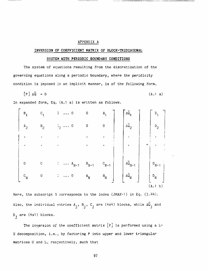
APPENDIX A
INVERSION OF COEFFICIENT MATRIX OF BLOCK-TRIDIAGONAL
SYSTSM WITH PERIODIC BOUNDARY CONDITIONS
The system of equations resulting from the discretization of the
governing equations along a periodic boundary, where the peridicity
condition is imposed in an implicit manner, is of the following form.
[P] AQ _ D (A.I a)
In expanded form, Eq. (A.I a) is written as follows.
B I CI S ... 0 0 AI
A 2 B2 32 ... 0 0 0
0 0 _ ... AN_ I BN_ I CN_ I
C N 0 S ... 0 AN BN
-AQI
AQ 2
AQN_ I
_QN
DI "lD2
DN- I
DN
(A.I b)
Here, the subscript N corresponds to the index (JMAX-I) in Eq. (3.44).
Bj . . andAlso, the individual entries Aj, , Cj are (4x4) blocks, while AQj
D. are (4xi) blocks.J
The inversion of the coefficient matrix [P] is performed using a L-
U decomposition, i.e., by factoring P into upper and lower triangular
matrices U and L, respectively, such that
97
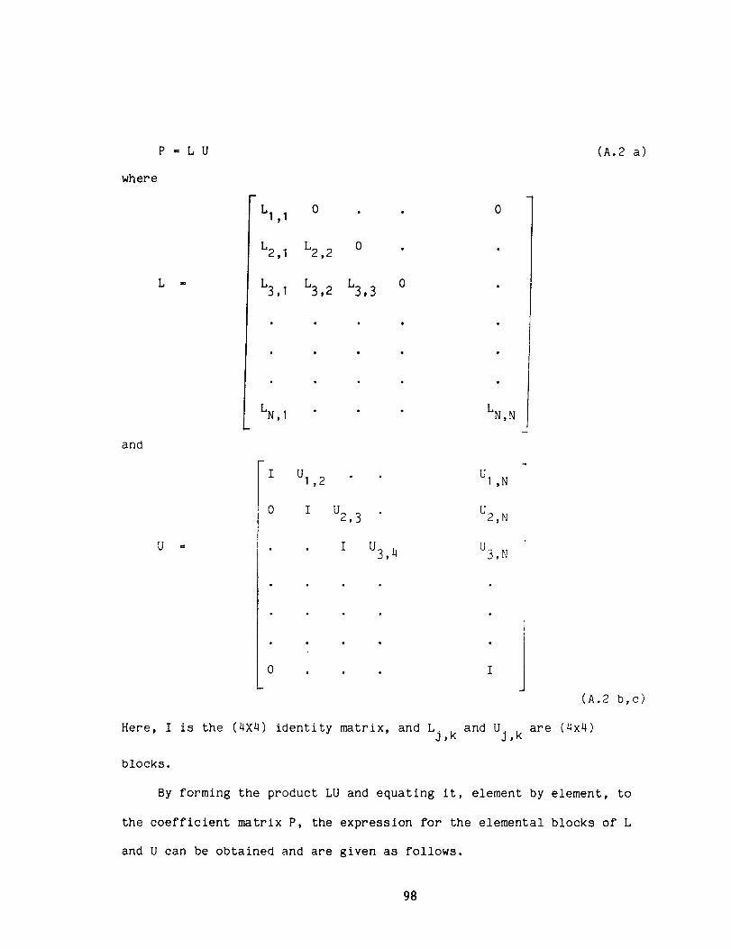
P_LU
where
L m
and
U
LI ,I O . .
L2, I L2, 2 O .
L3, I L3, 2 L3, 3 0
LN,I
I UI ,2
0 IU2,3
I U3, 4
LN,N
UI ,N
U2, N
U3,N
!
• • • I
J0 . . . I
(A.2 a)
Here, I is the (4X4) identity matrix, and L and U.j,k j,k
blocks.
(A.2 b,c)
are (4x4)
By forming the product LU and equating it, element by element, to
the coefficient matrix P, the expression for the elemental blocks of L
and U can be obtained and are given as follows.
98

L1 1 =BI
L2, I = A 2 ,
L3, L4 = LN_ I =I = ,I = """ ,I 0
LN, I = CN ,
-1
U1,2 = B1 C1
UI = U I = = UI = 0,3 ,4 "'" ,N-I '
-I
UI, N = B I A I
-I
L2, 2 = B 2 - A 2 B I C I
L3,2 = A3 '
= L5, = ... = LN_ I =L4,2 2 ,2 0
-I
LN, 2 = - C N B I C I
-I -I
U2, 3 = (B2 - A 2 B l C l) C 2
U2,4 = U2, 5 .... = U2,N_ 1 = 0
-I CI)-I A2 B?I AIU2, N = - (B2 - A 2 B I
etc.
Hence, the inversion of P is carried out in two steps.
step is a forward elimination step in which the equation
Lq=D
is solved for q.
This is done in the following manner.
(A.3)
The first
(A.4)
99
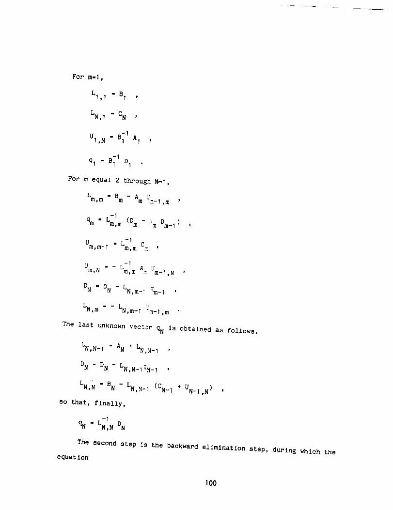
For m-1 ,
LI ,I = BI '
LN, I " CN ,
ql " B1 1 D1 .
For m equal 2 through N_I,
- Um_ ILm,m " Bm Am ,m '
qm " L-I (Dm - A D ) ,m,m m m-1
-IU - L Cm,m+1 m,m .T.
-I- A
Um,N - Lm,m - Um-I,N
DN = DN - LN,m-_ qm-1
LN,m " - LN,m-I "m-l,m
The last unknown vect:r qN is obtained as follows.
LN,N_ I " AN _ LN,N_ I '
DN - DN - LN,N_IqN_ I ,
LN, _ " B N - LN,N_ I (CN- I + UN_I, N) ,
SO that, finally,
qN " L-I DNN,N
The second step is the backward elimination step, during which the
equation
tO0
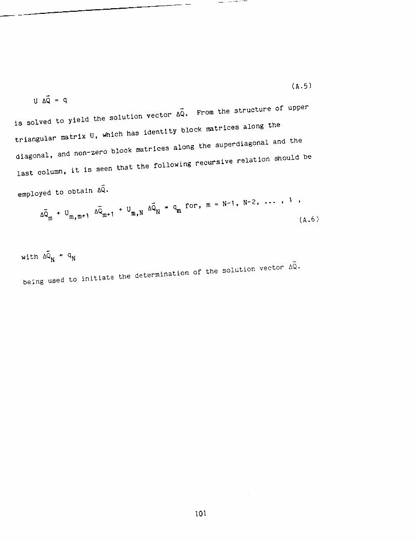
u = q (A.5)
is solved to yield the solution vector AQ. From the structure of upper
triangular matrix U, which has identity block matrices along the
diagonal, and non-zero block matrices along the superdlagonal and the
last column, it is seen that the following recursive relation should be
employed to obtain AQ.
+ U AQ + Um AQ _ for, m = N-I, N-2, IAQm m,m+1 m+1 ,N N qm "'" ' '
with AQN = qN
being used to initiate the determination of the solution vector AQ.
(A.6)
101

APPENDIX B
REPRESENTATION OF THE METRIC COEFFICIENTS
The metric coefficients, arising due to the transformation of the
governing equations from the physical (x,y) coordinates to the
computational (_,n) coordinates, should be evaluated in a manner
consistent with the discretizatlon of the governing equations.
The metric coefficients for a general mapping are given in Eq.
(2.13) and are
_x _ J Yn ' _Y _ - J Xn '
nx = - J y_ and ny _ J x_ . (B.I a-d
The metric derivatives xn and Yn are evaluated using central
differences at a general interior computational point (i÷1,j). Hence,
x I -- (xi+ - X )12Ann i+1,j I,j+I i÷I,j-I
and Y_li+1,j -- (Yi+1,j+l - Yi+I,j-I )/2An " (B.2 a,b
At a boundary point, these terms are evaluated using a first-order
accurate representation. Accordingly,
At j = JMIN,
xqli+1, j _ (xi+1,j+ I - xi+1,j)/An ,
Ynli+1, j I (Yi+1,j+1 - Yi+1,j )/An '
and, at j _ JMAX,
x I -- ( - )/An ,n i+l ,j Xi+l ,j Xl+1 ,J-1
YnIll+1,J " (Yi+1,j - Yi+I,J-I)/An • (B.3 a-d)
102

In order to determine the appropriate representation of x_ and y_,
a simple test of uniform-flow computation is employed. This test
involves assuming a uniform flow at a streamwise location i and applying
the numerical integration algorithm, along with uniform-flow boundary
conditions, to obtain the solution at station (i+I). If the algorithm
is formulated consistently, a uniform flow should result at station
(i+I)° To this end, it is sufficient to consider the inviscid part of
the governing equations, i.e.,
_E + 8F_-_ _ _ 0 (B.4)
since G-derivatives appear only in the Streamwise convective and
pressure-gradient terms. The quasi-linearized form of the above
equation can be obtained from Eqn. (3.27) and is
where
*iS = E
Here,
*iE =
and
_i _i_) : s
• . nx . ny _,
(B.5 a,b)
(B.6)
]03
Following the discretization procedure, as discussed in Chapter 3,
for the inviscid terms, the discretized form of the right-hand side of
Eqn. (B.5 b) at location (i+1,j) can be written as
I (5]i r_x]i+1 -*i (Cyli {_y]i+1 - "
1 r_x]i _xli+l -*i r_y]i _ (_yli+l -*i+ _ [{['J--'j+1 - [J--'j*1 ] Ej+I + [t_-'j+1 J 'j+1 ] Fj+I}
÷ 1]"J 'j-1 "J "j-1 Ej-I "<J--Jj-1 "J "j-I Fj_I
+ _ _Dx]i+I -*i _ (t]x]i+l -*iA_ {'J--'j-1 ej-I J--'j-1 Ej-I2 An
iny)i+l -_i _ "+ -_i
In order to recover a uniform-flow solution, it will be sufficient
to show that the source term S is zero, starting from uniform-flow
conditions at station i, and using uniform-flow boundary conditions. To
show this, it is recognized that, for the case with constant density,
velocity and temperature,
P = Pl
U = U 1
V- 0
and T - T I
where p,, u, and T, are constants.
with respect to the n direction, i.e.,
j-I = = , for j _ JMIN+I, ... , JMAX-I
-*iand F. = 0 , for j = JMIN .... , JMAX . (B.9)
J
104
Hence, the flux vectors are constant

With these conditions, the source term S can be written in the
following mannner.
I _h]i _xs _ {_ [ - (_-Ii+_]"J ,j j
+_[ - ,"J "j+1 _J "j+1 _J "j-1 _T'j-I ]
A_ [(___x)i+l _ rqx]i+l • (B.IO)
Substituting for (_x/J) and (qx/J) from Eq. (B.I) and employing the
discretization given by Eq. (B.2), Eq. (B.IO) can be written as
S = { 4_ [ - Yi+l,j+l - Yi+l,j-1 ) + (Yi,j+l - Yi,j-1 )]
+ _ [ - :i+l,j+2 - Yi+l,j ) + (Yi,j+2 - YL,j )
- vi+1 ,j - Yi+1 ,j-2 ) ÷ (Yi,j - Yi,j-2 )]
(B.11)
For S to be equal to zero, it is clear, from the above equation,
that y_ is to be evaluated, as an average of its neighbours, as follows.
I
Ygli+l,j+l " _ [Yi+l,j+2 - Yi,j+2 + Yi+l,j - Yi,j ]
1
+ -- [Y j+ - Yi ] (B.12)2 A_ i+I, I ,j+1
Similarly, by assuming v = constant and u = O, we can arrive at the
following representation for the term x_.
lOS

i I _ + xi _ xi ]x_ i÷l,j+l : _-_ [xi+1,j*2 xi,j+2 ÷l,J ,j
I
+ 2 [xi+ ,j÷1- xi,j÷1] (B.13)
The representation of x_ and y_ at q = constant boundaries, for
example, at j = JMAX can be obtained by forming the discretized form of
Eq. (B.5 b) at j = JMAX-I.
At the location [i+l,j (= JMAX-I)], the source term is written as
follows.
s--{ I_-_ [ - (Yi+1,j+1 - Yi+I,J-I ) + (Yi,j+I - Yi,j-I)]
I
+ _ [ - (Yi+I,j+2 - Yi+1 ,j ) + (Yi,j+2 - Yi,j )
- (Yi+1,j - Yi+1,j-2 ) + (Yi,j - yi,j_2)]
2 Aq 1,j+l 2 A_ Yi+1,j-1
l (Yi+ " y +4 At l,j i,j Yi+1,j-2 - Yi,j-2)] (B.I_
In order to produce a zero source term S, from Eq. (B.14), y_ term
should be represented in the following manner:
Y_li+1,j = JMAX " (Yi+1,j - Yi,j ) / A_ . (B.15
Similarly, the discretization for the term x_ is performed as follows.
X_li+1,j = JMAX = (Xi+1,j - Xi,j] / At(B.16)
]O6

APPENDIX C
DISCRETIZATION OF DERIVATIVES AT CORNERS OF FIVE_SIDED CELLS
In a hybrid grid, 'special-points' commonly occur at the congruence
of more than two different types of sub-reglons. As stated in Chapter
5, these 'speclal-points', B" and E" in Fig. 31, are presentlyc c
considered to be the centers of non-standard 5-sided cells. In the
discretization of the various derivative terms in Eq. (5.1), special
consideration is required in arriving at the appropriate neighbours for
the vertices of these 5-sided cells, i.e., in defining the computational
molecule at the vertices of these cells. The vertices of these non-
standard cells are B_' , B_ , ... , B_ and E_' , E2," ... , E_ , as shown
in Fig. 31. The eight immediate neighbours for each of these points are
shown as the encircled points in the sketches'below.
At vertex B_ , At vertex B_ ,
]07
At vertex B_ , At vertex B'_ ,
At vertex B_ ,
® immediate neighbours
The computational moleclues shown were arrived at by examining the
multi-block structured computational region and seeking the natural
neighbours of a given computational point. The neighbours at the
corners of the cell around E" are assigned in a similar manner. At ac
given vertex, the computational molecule employed during one step of the
two-step solution procedure, for the grid-generation equations as well
as the flow equations, is the same as that for the second step of the
procedure. This is essential for consistency of the discretized
equations used during the two steps.
IOB

,,-I
I-,I
ZO
Xr_
[...,i,.,..i
Zz
0r.,.
f-,.,
" d
0
m zQ 0
f._ u
_ m
III
0 I
o I
4..3 ,,_ 1.0
.c: nO I_.-, t-."
C3 • I_ 0
E I,-.4 1
E _ I•.-4 E: I
cD I
O c:L ...-4 I
I
Cj O I L
.._ ed I,._ E
•_ 0 I _ O
IIII
i..,
oo ooo o I,_o 0_J 04o o o
o o o
o o o
o ch oo,J o,J '4D
o o
c._ co•.,- 04
109
L
1,4I
0
! °
[
0
0O_
0
_,._
H0
lI
!I
!I
lI
°l0
I
!
II
i!
II
_!
0I'-I
Z0
r.1
tD
0
m_c_}
110

u,v,T
/////I///////I/I/////II/Iw
c x
• c,x,y,e
• c,x,y,e
• c,x,y,eY x
IIIIII/II/I/2//IIII/I/IIu,v,T
5
4
3
2
1
NO. OF UNKNOWNS
2O
TOTAL
NO. OF EQUATIONS
4 CONTINUITY
3 x-MOMENTUM
(3+I) y-MOMENTUM
3 ENERGY
6 BOUNDARY
CONDITIONS
20
WALL-WALL BOUNDARY CONDITIONS
/////////H///_///// , 5
c,x,y,e, 4
c,x,y,e, 3
c,x,y,e, 2
c,x,y,e 1I/II/I//IIII/I////II
0
NO. OF UNKNOWNS
16
TOTAL
NO. OF EQUATIONS
4 CONTINUITY
4 x'MOMENTUM
4 y-MOMENTUM
4 ENERGY
16
b. WAKE-WAKE BOUNDARY CONDITIONS
FIG. 2. TYPES OF BOUNDARY CONDITIONS FOR CASCADE FLOWS.
111

u,v,T
/I//////////I/////I/////
Yx• c,x,y,e
• c,x,y,e
• c,x,y,e
c,x,y,e
/Ii//////iii/////////i•cx
Q
u,v,T (lagged)
5 NO. OF UNKNOWNS NO. OF EQUATIONS
4
5 CONTINUITY
324 4 x-MOMENTUM
2 (4+I) y-MOMENTUM
1 4 ENERGY
6 BOUNDAHY
0 CONDITIONS
TOTAL 24
e. WALL-WAKE BOUNDARY CONDITIONS
p,u,v,T/////////// , 5 NO. OF UNKNOWNS NO. OF EQUATIONS
• c,x,y,e 45 CONTINUITY
• c,x,y,e 3 24 4 x-MOMENTUM
• c,x,y,e 2 4 y-MOMENTUM
c, x, y, e 1 4 ENERGY
27/ 7 BOUNDARY
, 0 CONDITIONS
u, v, T TOTAL 2_
d. WAKE-WAKE BOUNDARY CONDITIONS (REGION-PERIODIC GRID)
FIG. 2 (CONCLUDED). TYPES OF BOUNDARY CONDITIONS FOR CASCADE FLOWS.
112

Inflow
Boundary
P
z i+l i+2
Outflow
Boundary
FIG. 3. TWO STEPS OF THE SOLUTION PROCEDURE.
Fully
DevelopedFlow
Profile
h=l
V
t/2
Constant
Static
Pressure
a. EXPONENTIAL CHANNEL
.... ////////////_////J//////
Uniform
VelocityProfile
h
///////#//#/x///#//////
Constant
Static
Pressure
b. FLATePLATE CASCADE
FIG. 4. CONSTRICTED CHANNEL AND VARIOUS CASCADE CONFIGURATIONS,
AND INFLOW-OUTFLOW BOUNDARY CONDITIONS.
113

Uniform
VelocityProfile
h
e. CASCADE OF EXPONENTIAL AIRFOILS
Constant
Static
Pressure
Uniform
Velocity
Profile
h
Constant
Static
Pressure
Uniform
VelocityProfile
d. CASCADE OF PARABOLIC-ARC AIRFOILS
q
h
Lem--_
t
Constant
Static
Pressure
e. CASCADE OF JOUKOWSKI AIRFOILS WITH MODIFIED LEADING EDGES
FIG. 4 (CONCLUDED). CONSTRICTED CHANNEL AND VARIOUS CASCADE
CONFIGURATIONS, AND INFLOW-OUTFLOW BOUNDARY CONDITIONS.
114

I
II|
III|
I!
IIII
! !
]
il
i
i :
ZI-I
[-,
ILl
I=
I--I
&I-I
,-I
I--I
i.-I
115

ia. 2{}
ia. is
8.1ia
Pb8, ias
la. iala
-{a. {3s
-_. 10
)
III, i I 1 I, J, I [ , , I
0 I_ X Z_ 38
-- ........................ PD (ii) !o
i
[_i
2 4 X 6 8
ENLARGED HORIZONTAL SCALE
{a,_5
Y
8.18
8 85
_}, [a{a
16.{} i
12.0
(iii)
LL ._,_J_LJ.. _LJ_...L.I..J__L..J__L_
g I0 X 20 3g
LLF5.LI
J
(iv)
' ...... J ' J ....... J --_
Z 4 X 6 8
ENLARGED HORIZONTAL SCALE
a. t/h = O. I
FIG. 6. WALL-PRESSURE AND WALL-SHEAR PARAMETER DISTRIBUTIONS
FOR EXPONENTIAL CHANNEL CONFIGURATION, Re - 1500.
116

0.4
0.3
0 2
Pb
0 I
0.0
-0. I
- (i)
b
0 _0 X 40 50
0.48
0,20
14 15 X 16 17
ENLARGED HORIZONTAL SCALE
0.10
0.00
40
30
20
TW
10
-10
E
(iii)
, ! i I ,,
0 20 X 40 60
i...... .......
, , , I I , i , J I , , , I
14 15 X 15 17
ENLARGED HORIZONTAL SCALE
b. t/h - 0.16
FIG. 6 (CONT'D). WALL-PRESSURE AND WALL-SHEAR PARAMETER DISTRIBUTIONS
FOR EXPONENTIAL CHANNEL CONFIGURATION, Re - 1500.
117

(i)
25 S0 x 75
m
I
(ii) --
100 27 28 29 X 30 31 32
ENLARGED HORIZONTAL SCALE
8 40
0.30
y
0.20
0.10
0,00
40
30
20
TW
10
0
-10
(iii)
m
0 25 $0 x 75 100
J
(iv)
, ] | [,,I, I ¢ ] i
27 28 29 X 30 31 32
ENLARGED HORIZONTAL SCALE
c. t/h = 0.2
FIG. 6 (CONCLUDED). WALL-PRESSURE AND WALL-SHEAR PARAMETER DISTRIBUTIONS
FOR EXPONENTIAL CHANNEL CONFIGURATION, Re - 1500.
118

O'I 8"0 9"0 _'0 C'O
,3
If9

E;'O
C_0
('0
C_
c_
O0CO
c_
Z'O I'0 0"0
O0o,-)
I"O- Z'"0-
u'_
_'0-
120

,z
I.I
(i)
I , l t
zs x 58
o Pbu
75
I
I (ii) oP b
I _U
!9 I_ x II Iz
ENLARGED HORIZONTAL SCALE
1.5
u
i
15Q ---i
I
•_lll --
5Q _--
Q
_SQ _.___L__
(iii)
Z5 x 58 7S
(iv)
, I , I i
9 I_ x II Iz
ENLARGED HORIZONTAL SCALE
a. Re = 1500
FIG. 8. WALL_PRESSURE, WAKE-CENTERLINE VELOCITY AND
WALL-SHEAR PARAMETER DISTRIBUTIONS FOR A CASCADE
OF FINITE FLAT PLATES.
121

Q.I !I
_.1_ , b----qN
-0, I --
i
-0, Z
(i)
, l , .i a
Z$ X 5_ 75
oP b
_U
9 18 X II IZ
ENLARGED HORIZONTAL SCALE
1.5
I.Q
u
zQ_ --
I_8 --
Tw
Q
9
(iii)
Z5 x 50 75
(iv)
|1_ x It IE
ENLARGED HORIZONTAL SCALE
b. Re - 3100
FIG. 8 (CONT'D). WALL-PRESSURE, WAKE-CENTERLINE VELOCITY AND
WALL-SHEAR PARAMETER DISTRIBUTIONS FOR A CASCADE
OF FINITE FLAT PLATES.
122
a.t
-Q, Z
I
m -
!
J I I
_8
(i)
7_ 9 t_ tt tZX
ENLARGED HORIZONTAL SCALE
I.K
u
208
IS0
IO{a
W
5ta
Q
(iii)
0 ZS 50 7SX
(iv)
! I i I ,
9 18 X II iZ
ENLARGED HORIZONTAL SCALE
e. Re - 6200
FIG. 8 (CONT'D). WALL-PRESSURE, WAKE-CENTERLINE VELOCITY AND
WALL-SHEAR PARAMETER DISTRIBUTIONS FOR A CASCADE
OF FINITE FLAT PLATES.
123

-8. Z
0
(i)
ZK x S8 7_
-_ _ "___ |
18 X _I IZ
ENLARGED HORIZONTAL SCALE
!
8
1,8
U
TW
ZC_0
188
$8
8
(iii)
....... --------..4...]
(iv)
8 18 x 11 t_
ENLARGED HORIZONTAL SCALE
d. Re - 11000
FIG. 8 (CONT'D). WALL-PRESSURE, WAKE-CENTERLINE VELOCITY AND
WALL-SHEAR PARAMETER DISTRIBUTIONS FOR A CASCADE
OF FINITE FLAT PLATES.
124
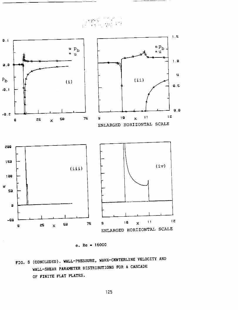
8.1
Pb
-0. I
-1_.Z
o PbU
(i)
ZS X 58 7K
o Pb
I :_ ! 1
9 18 X 11 tZ
ENLARGED HORIZONTAL SCALE
I.S
1.g
U
I_8
Iso
w5o
(iii)
8 Z5 x KS 78
(iv)
, I z I L
g tO X tt IZ
ENLARGED HORIZONTAL SCALE
e. Re - 16000
FIG. 8 (CONCLUDED). WALL-PRESSURE, WAKE-CENTERLINE VELOCITY AND
WALL-SHEAR PARAMETER DISTRIBUTIONS FOR A CASCADE
OF FINITE FLAT PLATES.
125
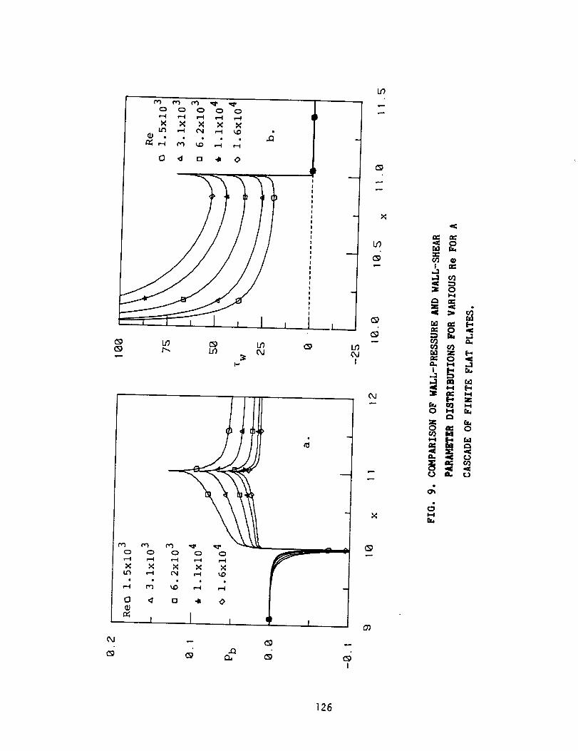
o o o_
o,I
IP) ,--I _ ,,-I _ •..... .CI
I_ <I o .(k <>
i I i i
(_ r-. I.F) oJ ou
I-,
I
tI
I.o
x
x
126
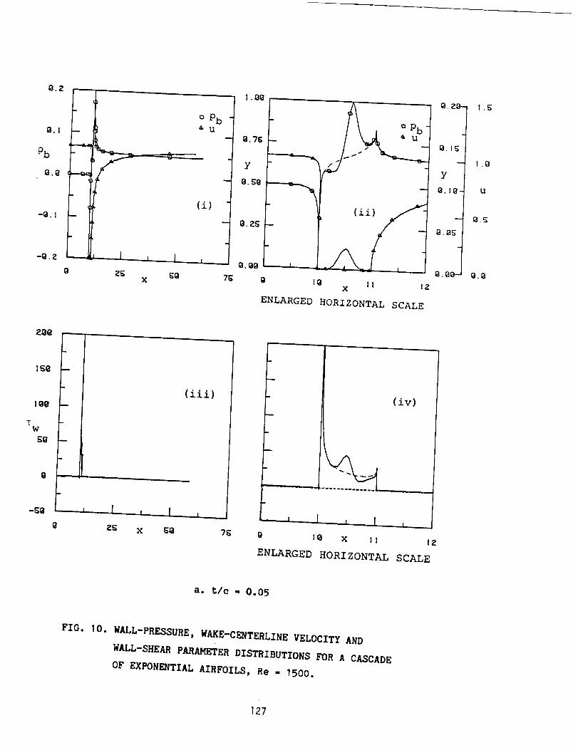
0.Z
01
_b
08
-81
-SZ
t
i
I , {
Z_ _8x
(i)
I
I • 08
8.7_
y
-- O. 58
8. ZS
8.88
7_
= ci -[I/k_
II fill II 12x
ENLARGED HORIZONTAL SCALE
O.Z8- I .5
8.1_
1.0
Y
0.18- u
- 0.5
8.80- 8.8
Z88
"cW
m
m
w
p
(iii)
"I
III
II
i!
I
I
I
I
II
2_ X _Q 7_
(iv)
, I i I
8 IQ X II I: _
ENLARGED HORIZONTAL SCALE
a. t/e - 0.05
FIG. 10. WALL-PRESSURE, WAKE-CENTERLINE VELOCITY AND
WALL-SHEAR PARAMETER DISTRIBUTIONS FOR A CASCADE
OF EXPONENTIAL AIRFOILS, Re - 1500.
127
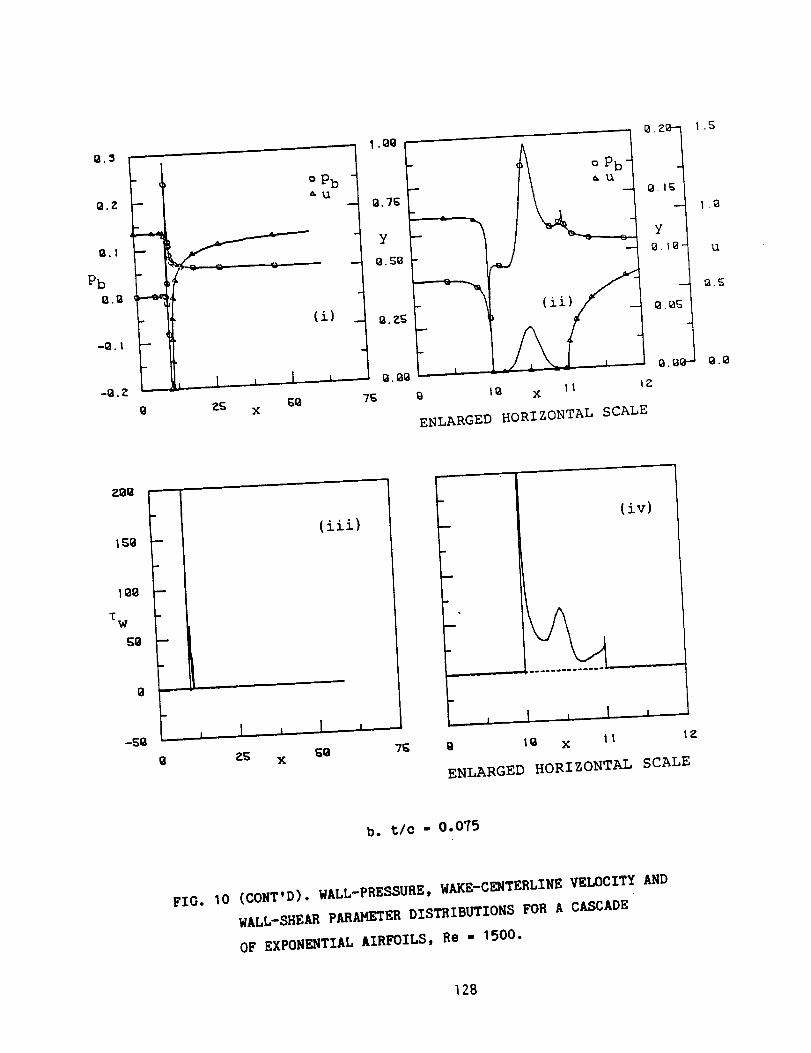
0. Z pub --
0.1
Pb
0.0
-0. ! _
-0. z
8 ZK x KO
I. 00 I_. z_-
I_ _ a Pb"i _ _u
8.7_ \ , - 8.1_ !
Y _ Y
O.5_ _ L 8. 10-
8. Z5 _, 85
8. I;_8 "_ - - "-' 8.88-
7_ _ 10 X II IZ
ENLARGED HORIZONTAL SCALE
I.S
1.8
U
_.S
IiI.8
TW
150
r"
0
i
-50
(iii)
ZK x _Q 7K
(iv)
10 x 11 IZ
ENLARGED HORIZONTAL SCALE
b. t/o - 0.075
FIG. 10 (CONT'D). WALL-PRESSURE, WAKE-CENTERLINE VELOCITY AND
WALL-SHEAR PARAMETER DISTRIBUTIONS FOR A CASCADE
OF EXPONENTIAL AIRFOILS, Re - 1500.
128
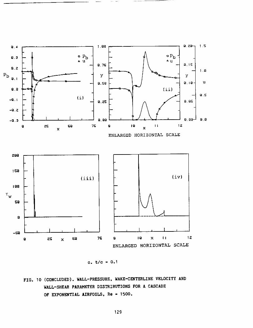
Pb
Q.4 I"
Q.3 --
_.Z t--
I
-Q. ! --I
r-Q. Z _
i-I
_Q. 3 i
9
(i)
I I, i l
ZE K_X
- Q. 7g
Y
- 13.59
- 8.Z_
__ _ o Pb
9 19 11 IZX
ENLARGED HORIZONTAL SCALE
8.Zmn I.5
o. lgl
1.9
Y
9.19-I u
8._g I
*-4
8.88-_ 9.8
TW
Z¢8
i
188 ---
FE8
9
-E9
I(iii) ,
____L_________ I0 Zg X E8 7g
(iv)
, I , I ,
g I_ x II IZ
ENLARGED HORIZONTAL SCALE
e. t/o - 0.I
FIG. 10 (CONCLUDED). WALL-PRESSURE, WAKE-CENTERLINE VELOCITY AND
WALL-SHEAR PARAMETER DISTRIBUTIONS FOR A CASCADE
OF EXPONENTIAL AIRFOILS, Re = 1500.
129
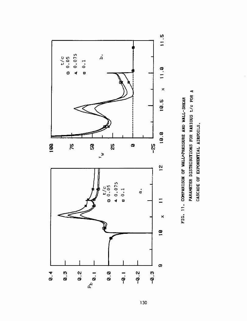
D.
"-- r_ n_ rJmm
xrL
N
I I I I I
I i I
130
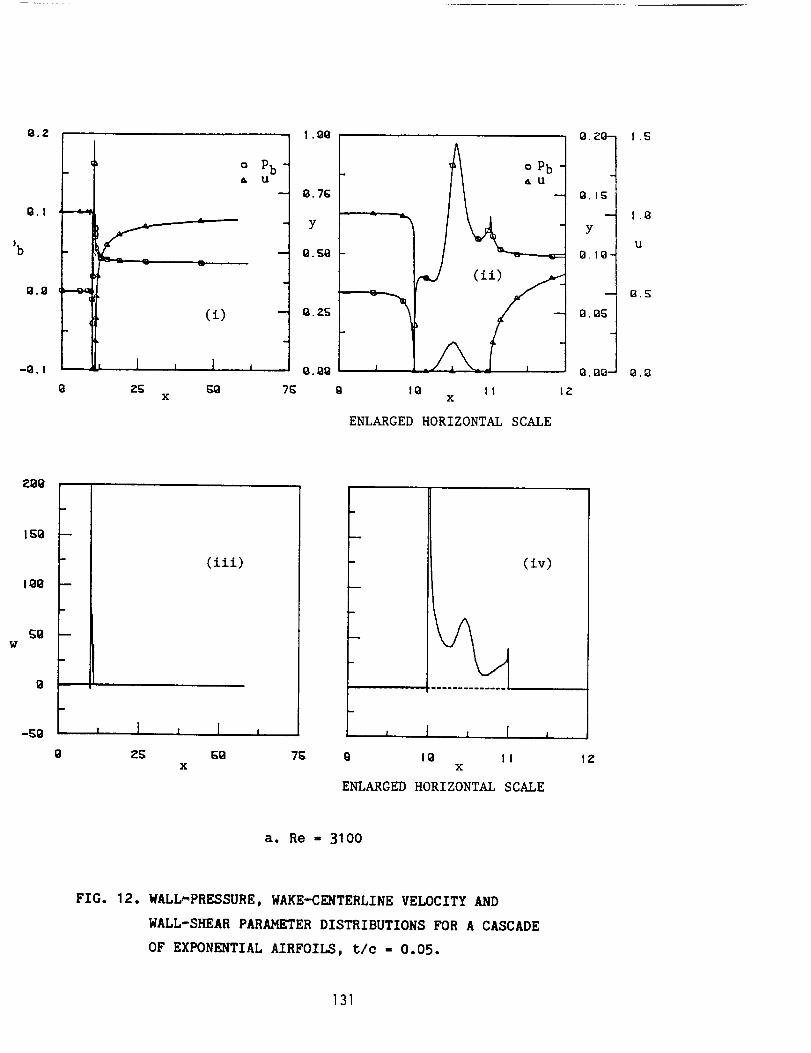
-Q. I
&
(i)
Zg g_x
o Pbu
1 • _
Q. 7G
x
ENLARGED HORIZONTAL SCALE
.
Y
13._.1_-
-- Q.E
w
:_QI_ --
Q
(iii)
2g g_ 7GX
(iv)
, I , I ,
9 II_ IIx
ENLARGED HORTZONT_J_ SCALE
IZ
a. Re - 3100
FIG. 12. WALL_'PRESSURE, WAKE-CENTERLINE VELOCITY AND
WALL'SHEAR PARAMETER DISTRIBUTIONS FOR A CASCADE
OF EXPONENTIAL AIRFOILS, t/e - 0.05.
131
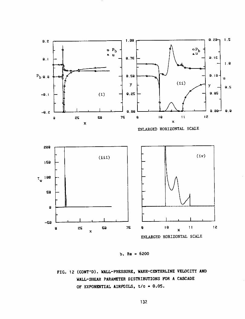
O Z
Pb _.o
-_. t
-_. z
q
i
, q
0
tl
f , l
Z_; KQ
x
(i)
o Pb
u
7K
1 •O0
Q. 71;
O. 59
Y
8. ='5
Q. QB
- 0
oP b
-- (ii_
G IQ II IZ
x
ENLARGED HORIZONT_ SC_E
O.Z_ 1.5
O,a_l
O. IO_u
Y -- o.S
O. tM;
t_. OO--- (a.8
aSS --
lSO --
T 10O --w
gO --
0 -'--
(±ii)
0 _ E;O 7gX
(iv)
9 I0 II 1::'x
ENLARGED HORIZONTAL SCALE
b. Re - 6200
FIG. 12 (CONT'D). WALL'PRESSURE, WAKE-CENTERLINE VELOCITY AND
WALL-SHEAR PARAMETER DISTRIBUTIONS FOR A CASCADE
OF EXPONENTIAL AIRFOILS, t/c - 0.05.
132

Q Z
-Q. !
-_ Z
i
o Pb_' U
(i)
J t [ t
2_ x gB
1 • QQ
g. 7_
y!
_. $0
0 Pb -'
_u g.l_]
--' 1._-y
"_ :3 U
-- 1_. i_
7£ g I_ II IZx
ENLARGED HORIZONTAL SCALE
0.8_ I
_. _t_.-- Q.ta
21ala
lgla
51a
-_ta
1
(iii)I (iv)
___x ]
9 IG 11 I::'X
ENLARGED HORIZONTAL SCALE
o. Re l 1 1000
FIG. 12 (CONT'D). WALL'PRESSURE, WAKE-CENTERLINE VELOCITY AND
WALL-SHEAR PARAMETER DISTRIBUTIONS FOR A CASCADE
OF EXPONENTIAL AIRFOILS, t/c " 0.05.
133

Pb
o.z
o.1
0.0
-0. I
-0. z
op bAU
Zg gO 7_X
o.zI_ I.s
I.O
I 13.S
I;3,_3S!
z O._3Q-- O.Q
g 10 It IZX
ENLARGED HORIZONTAL SCALE
TW
2Q0
I_
_Q
8
(ill)
0 2_ x 6_ 7_ 0 10 x II IZ
ENLARGED HORIZONTAL SCALE
d. Re - 15000
FIG. 12 (CONCLUDED). WALL,_PRESSURE, WAKE-CENTERLINE VELOCITY AND
WALL'SHEAR PARAMETER DISTRIBUTIONS FOR A CASCADE
OF EXPONENTIAL AIRFOILS, t/c " 0.05.
134

I
_8
_ z
g
135

!
!
0Q
|
0
|
0
136

X X "_
_ _--"
:
_, I , I ,I
I
I
.Q
5")
i
._ _: 0
o
r_
, o _
x
_ H
z o
H
m
137

Pb
O Z
0.1
gO
-13. I
(i)
o Pbu
1 t [ J
X
I . O0
0.7_
Y
0. SO
-- 0.2_;
i
i o._{}
7S 8 18 II 1Zx
ENLARGED HORIZONTAL SCALE
O. Z_-
0.I_
la. lla-
O. O_
.
O. 013-
1.0
U
0.8
TW
!
I _8 t-.
L108 _-
F5_ L-
It"
o I----
(iii)
__L___.__
ZS EO 7S 8
x
(iv)
i I , I ,
18 IIx
ENLARGED HORIZONTAL SCALE
a. tic - 0.05
FIG. 15. WALL-PRESSURE, WAKE-CENTERLINE VELOCITY AND
WALL-SHEAR PARAMETER DISTRIBUTIONS FOR A CASCADE
OF PARABOLIC-ARC AIRFOILS, Re - 1500.
138

Z
3
b _ Pb,t U
0 Q
•_ "_l (±)
i|
Q :'5 _X
1 • O0
._ Y
7_
I
9 I1_! x It l_
ENLARGED HORIZONTAL SCALE
I;I.Zl_--1 1.-_
o Pb __
B,IEI
U
•--.., O.g
_.og I
_. o_--_ _._
ZQQ
150
15)O
Tw
5O
0
-gO
(il:i)
, I I i ,
Z5 50X
75 9
B
i
m
m
(iv)
, I J I ,
18 IIX
ENLARGED HORIZONTAL SCALE
12
b. tlc = 0.075
FIG. 15 (CONY'D). WALL_PRESSURE, WAKE-CENTERLINE VELOCITY AND
WALL-SHEAR PARAMETER DISTRIBUTIONS FOR A CASCADE
OF PARABOLIC-ARC AIRFOILS, Re - 1500.
139

Pb
Q.S
O Z
Q.I
98
-@.!
-Q. Z
I
m
m
= PbA u
(i)
I , 90
O. 7t;
Y
Q. 25
Z5 _Q 75x 18 x I I IZ
ENLARGED HORIZONTAL SCALE
ZOI3
"Tw
150
I O0
58
0
-_9
m
p-
(iii)
0 Z5 x 5Q 75 9
(iv)
, I , I ,x
18 II
ENLARGED HORIZONTAL SCALE
12
o. 1;/o = 0.1
FIG. 15 (CONCLUDED). WALL-PRESSURE, WAKE-CENTERLINE VELOCITY AND
WALL-SHEAR PARAMETER DISTRIBUTIONS FOR A CASCADE
OF PARABOLIC-ARC AIRFOILS, Re = 1500.
140
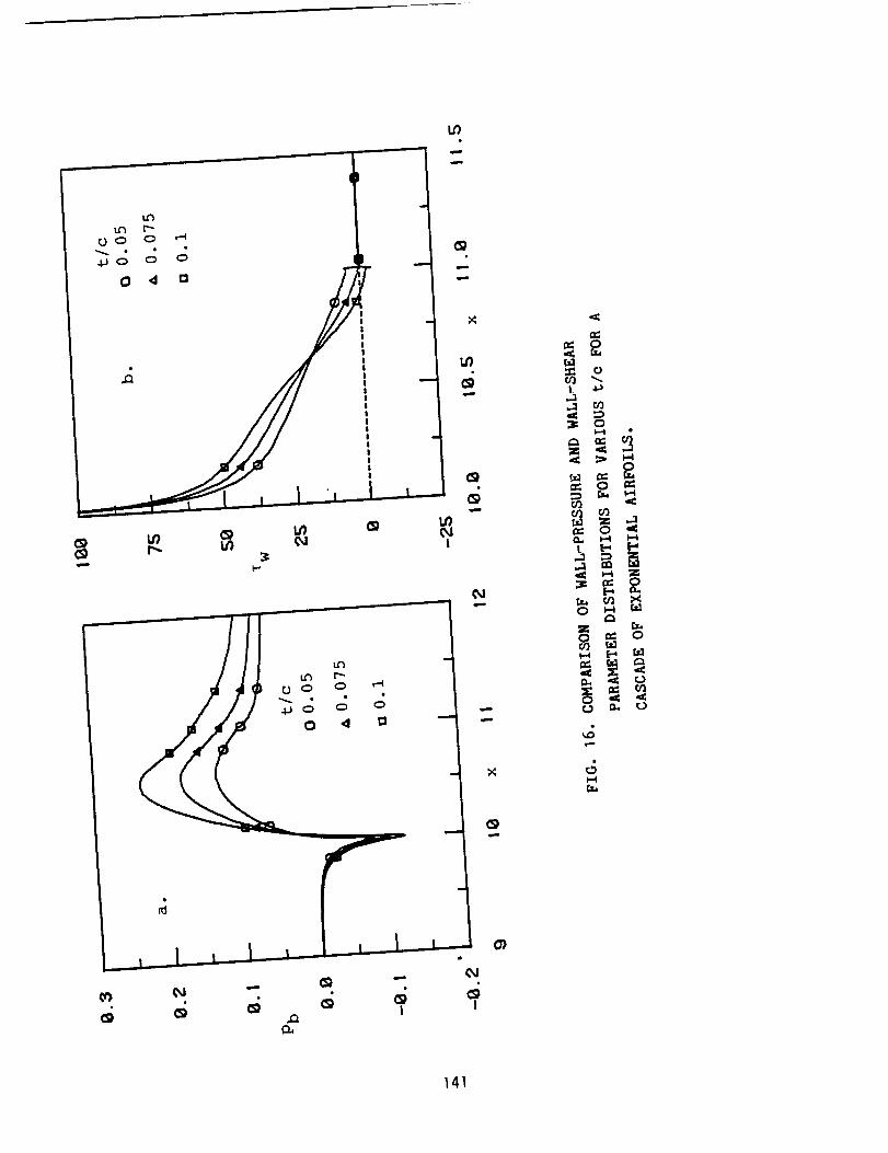
bO
O)
141

8.Z
g.8
Pbak
u
- f___--- -- 0 Q
Q Z5 5Q
(±)
7_
I •I_
I_. 76;
y
8.2_
t oPbtALl.
| .... 1
18 II l_X
ENLARGED HORIZONTAL SCALE
g. Zg-
Y
Q.IB-
m
_. OS
Q. _1_
1.5
I.la
U
_.S
W
Zgg F-- "rl
I
I _g f
I
t-
p.
Z5 x gQ 7N
m
(iv)
, I L I ,
IQ x It
ENLARGED HORIZONTAL SCALE
t2
a. Re - 3100
FIG. 17. WALL-PRESSURE, WAKE-CENTERLINE VELOCITY AND
WALL-SHEAR PARAMETER DISTRIBUTIONS FOR A CASCADE
OF PARABOLIC_ARC AIRFOILS, tlc - 0.05.
]42

Pb
o.z
Q.l
Q.g
-43.t
q
Q
(±)
Q Pb4 i/
I ._ ,
Q.7S t
Y
7_
g. _Q
Q. 2_
I_ x II t_
ENLARGED HORIZONTAL SCALE
Y
G.IG-
g. g_;
.
8.89"-
I.E
I.la
U
..[W
ZQQ -'-'----
1_Q(ili)
S_
s
i
J__ t_
ZE x EQ 7_
w
(iv)
, I ...i I .,.
I_ x II
ENLARGED HORIZONTAL SCALE
b. Re = 6200
FIG. 17 (CONT'D). WALL'PRESSURE, WAKE-CENTERLINE VELOCITY AND
WALL'SHEAR PARAMETER DISTRIBUTIONS FOR A CASCADE
OF PARABOLIC-ARC AIRFOILS, t/C - 0.05.
143
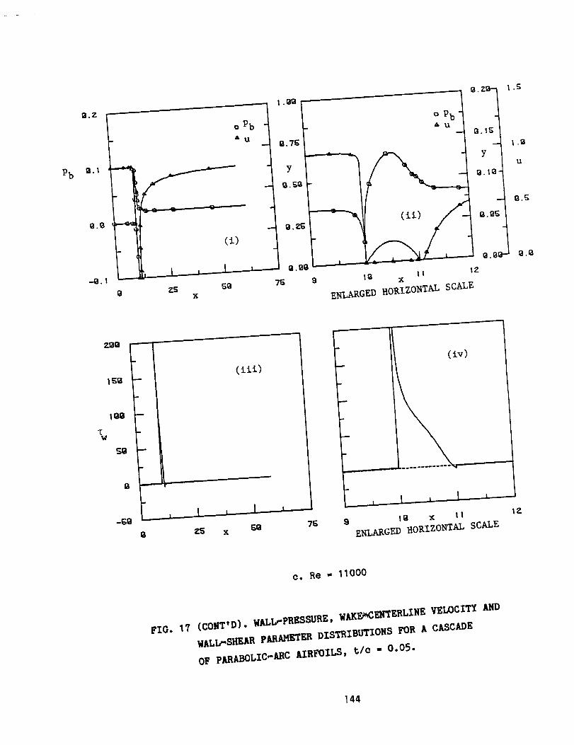
t_.zo--1 I .sQ.z I .rill .
Q._Q Q. 1
•,-O. 1 I , Q.BO " _ -_":- "- :--- " " " _.6_P- O,B
0 Zg 5Q 75 9 ! 0 t I I ZX X
ENLARGED HORIZONTAL SCALE
I
5Q --
0
(±i±)
='5 x 5Q 75
I
m
(iv)
I
8 tO x tl lZ
ENLARGED HORIZONTAL SCALE
e. Re - 11000
FIG. 17 (CONT'D). WALI_PRESSURE, WAKF_CENTERLINE VELOCITY AND
WALL_SHEAR PARAMETER DISTRIBUTIONS FOR A CASCADE
OF PARABOLIC_ARC AIRFOILS, t/O - 0.05.
144
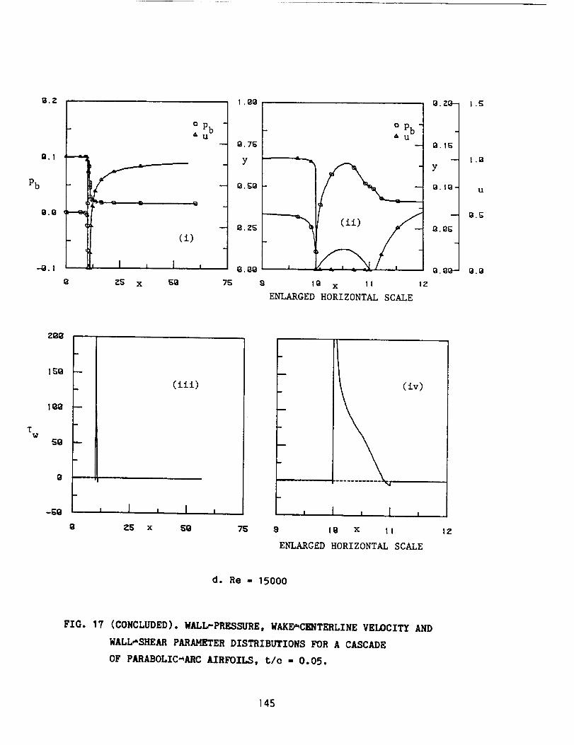
Q.Z
-Q. t
i
°
I
!
i
PbU
I . 01_ ,
8.7G 1
y _
ca.gQ
- la. 2_
(i)
I I I , 9. Og
Z5 x _0 75 8
(ii)
lg x I I lz
ENLARGED HORIZONTAL SCALE
o.z_ I .5
--4
l_.1_ I
1.1]Y
Q.tgg uI
1_.80-- I_.O
TW
z_,a F q
_Q L.- I|
Io
(ill)
Z5 x _0 75
1
I
(iv)
, I , I ,
8 IO x II
ENLARGED HORIZONTAL SCALE
12
d. Re - 15000
FIG. 17 (CONCLUDED). WALL'PRESSURE, WAKE_CENTERLINE VELOCITY AND
WALL_SHEAR PARAMETER DISTRIBUTIONS FOR A CASCADE
OF PARABOLIC_ARC AIRFOILS, t/O = 0.05.
145
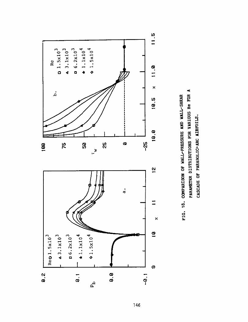
LO
u
7
I ,
ix
.c
146
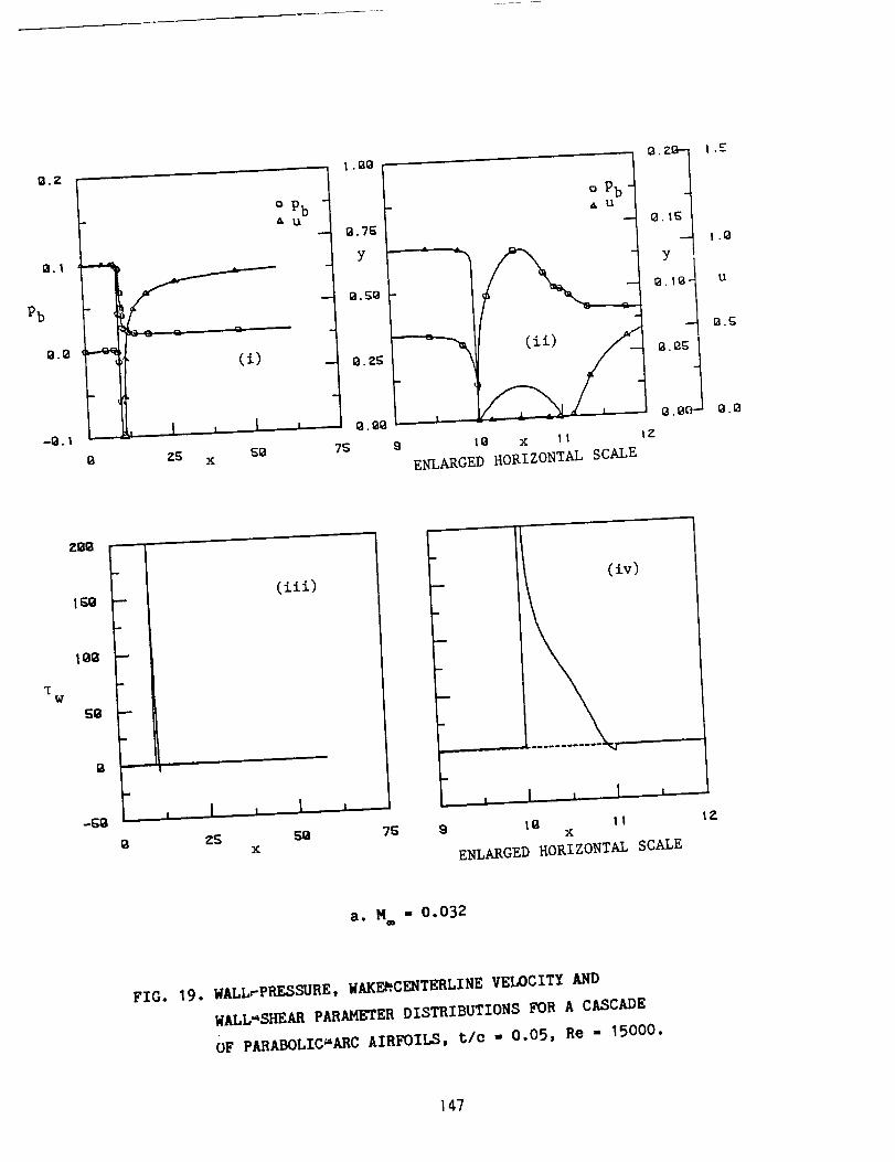
Q.Z
Pb
q
g
I
S(i)
I , I
Z5 5_x
o PbA U
I
! . 130
-- cl 7g
Y
-- 1_. 2S
O. gg
75 9 IQ x I I IZ
ENLARGED HORIZONTAL SCALE
B,Z_ I .r
o Pbu
_._I
•-_ 1.13
Y
(3. I(3 t u
13'0g t
.... g, gO ---_ g.13
TW
ZI_Q
1_o
IoI_
5_
r_
|
k.,,
I
L_
i
Ii
(iii)
Z5 5Q 75 9x
m
I
i
]
I
iv) III
I
I
III
I
I
IQ IIx
ENLARGED HORIZONTAL SCALE
IZ
a. M - O.032
FIG. 19. WALL_PRESSURE, WAKF_.CENTERLINE VELOCITY AND
WALL'SHEAR PARAMETER DISTRIBUTIONS FOR A CASCADE
OF PARABOLIC_ARC AIRFOILS, tlc - 0.05, Re - 15000.
147
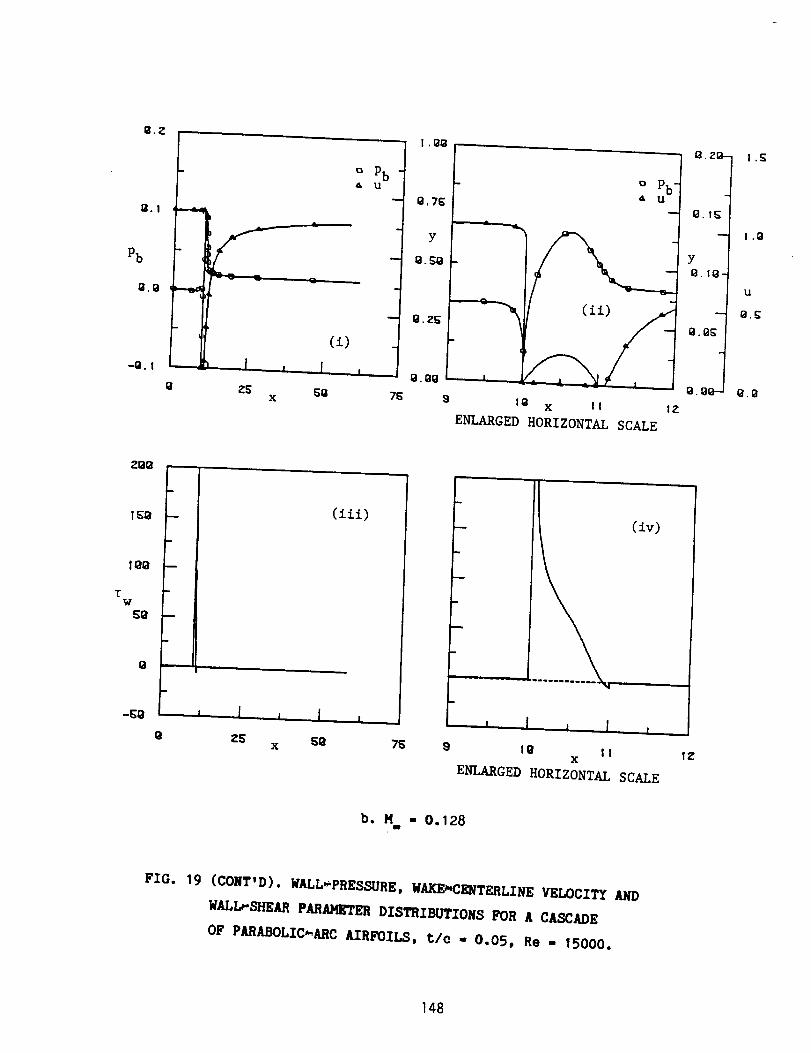
O.Z
B.I
--O.1
0
o PbA u
Z5 S8 75 9x
Q. ZO--
_.1_
(il)
tZ18 x II
ENLARGED HORIZONTAL SCALE
Y
ta. tS-
1.5
U
8,0
Z88
1O0
Tw
SO
-£0
(iii)
• Z5 5_ 7_ 9x
m
(iv)
, l ,, l ,
tO ttx
ENLARGED HORIZONTAL SCALE
IZ
b. M = 0.128
FIG. 19 (CONY'D). WALL_PRESSURE, WAKE_CENTERLINE VELOCITY AND
WALLrSHEAR PARAMETER DISTRIBUTIONS FOR A CASCADE
OF PARABOLIC_ARC AIRFOILS, t/o - O.05, Re - 15000.
148
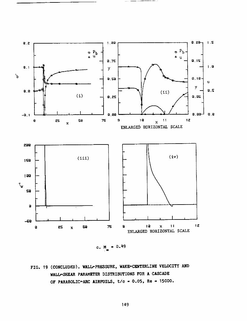
'b
o z
Q.I
-Q. I
(±)
, I , , ]
g Z5 SQx
o PbA u
I •fig
g. 7E
Y
Q.SQ
°pbt
(ii)
tO f;x
ENLARGED HORIZONTAL SCALE
tZ
Q.ZQ--1 1 .5
O.tSI
O. 10-1u
Y
Tw
ZQO
! O0
SO
-£,g
m
m
i
(ill)
0 Z5 x _0 7S
m
(iv)
9 I0 x It IZ
ENLARGED HORIZONTAL SCALE
C. M = 0.49
FIG. 19 (CONCLUDED). WALL_PRESSURE, WAKFrCENTERLINE VELOCITY AND
WALL_SHEAR PARAMETER DISTRIBUTIONS FOR A CASCADE
OF PARABOLIC_ANC AIRFOILS, t/o - 0.05, Re - 15000.
149

00 ur_0 ¢_ _ oh
o o o o
, I _ I s I ,
1'_ It) _1
t-'
1
I
IZ)
m
x
Lt)
m
m
x
m
O)
,r $
r.,fj u
i-i
150

I1i
t
I I
I
! |
i
1
/
NO.
!
2
3
5
6
?
8
9
l0
II
12
13
15
16
17
18
19
20
21
VALUE
0.29226E0.29313E
0.2?q-OOE
0.29_87'E
0.2957q-E
0.29662E
0.297'_9E0.29836E
0.29723E
0.300] ]E
0.30098E0.30185E
0o30272E
0.30359E
O. 30'_,?E
0.3053_-E
0.30621E0.30708E
0.30796E
O,30883EO.30970E
01
oJ
01
O!
OJ
Ol01
O!
O]
OJ
OlO!
01
O]
01
Ol
O]OJ
OJ
01oJ
FIG. 21. STATIC PRESSURE CONTOURS FOR A CASCADE OF
PARABOLIC_ARC AIRFOILS, Re - 15000, M® - O. 49.
15l
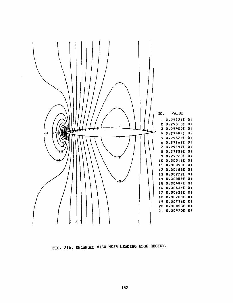
///
I
NO. VALUE
! 0.29226E OJ
2 0.293_3E O]
3 0.29_00E O]
? _ 0.29_FB?E OJ
5 0.2957qE 01
6 0.29662E 03? 0.297_9E Ol
8 0.29836E Ol
9 0.29923E 01
lO 0.3001 1E Ol
11 0.30098E 01
12 0.30185E 01
13 0.30272E 01
I+ 0.30359E Ol
15 0.30q_TE 01
16 0.3053_E 0112 0.30621E Ol
18 0.30708E 01
19 0.30?96E 01
20 0.30883E 01
21 0.30970E 07
FIG. 21b. ENLARGED VIEW NEAR LEADING EDGE REGION.
152

153
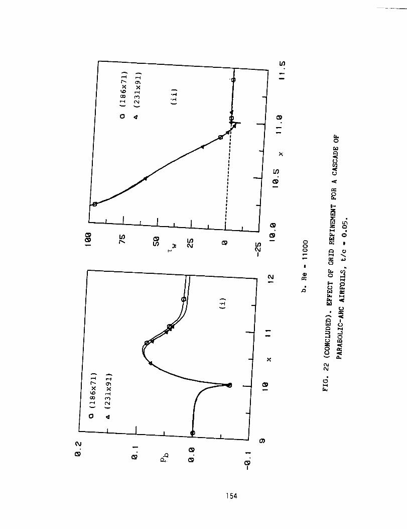
.Q
/-.
m
m
m
o0ov--
q..
I
0
c_
Z 0
o
O
dQ _
E-,
IN
154
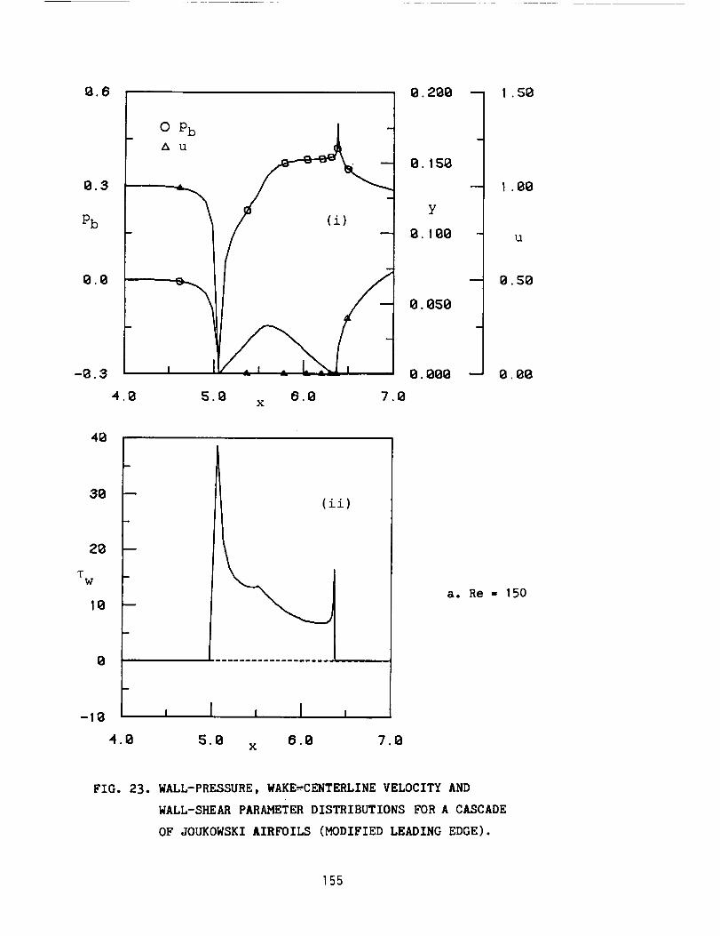
Pb
0.8
-8.3
4.8
O Pb
A U
5.0X
(i)
8.0 7.8
8.158
0.858
0.088
-- I.88
U
-- g. 58
-- 8.88
40
20
TW
10
m
38 --
0
-10
4.8 5.8
(ii)
8.0 7.8X
a. Re - 150
FIG. 23. WALL-PRESSURE, WAKE_CENTERLINE VELOCITY AND
WALL-SHEAR PARAMETER DISTRIBUTIONS FOR A CASCADE
OF JOUKOWSKI AIRFOILS (MODIFIED LEADING EDGE).
155
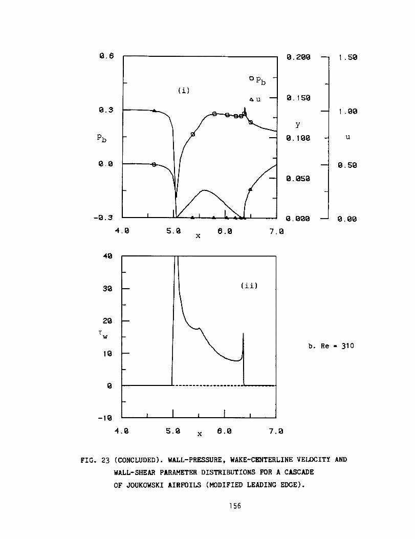
0.6 0.280 -- 1.50
0.3
Pb
1_.0
-0.3
(i) °Pb
ALl
4.0 5.0 8.0 7.0X
0. 158
8. 050
0. 800
-- 1. gO
- U
-- g. 58
-- 8.00
4g
30
20
TW
10
0
-10
(ii)
mL L i_
4.8 5.0 x 8.0 7.0
b. Re l 310
FIG. 23 (CONCLUDED). WALLIpRESSURE, WAKE-CENTERLINE VELOCITY AND
WALL-SHEAR PARAMETER DISTRIBUTIONS FOR A CASCADE
OF JOUKOWSKI AIRFOILS (MODIFIED LEADING EDGE).
156

I
)IIIII I I I
w w
0 <f
IIIII i I
,-4
I _ I
lili I i I I
I I I
lllll I I i
i I
lllll I I i I _I
I I
I
1.4
0nn
f._o
LO
-m cJ_ u
•,--i _
o =
I.) ,_
157
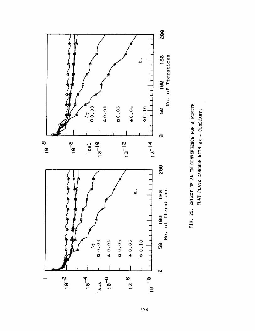
4-)
-l-J
o
I I (n I I --
@ (:_ ,_ @ @ I
uJ
£-.I--I
_-_ Z
00 r_
IIra_
°_
Od
I-q
158

I_ _ I I I
_"iX
<_I_
,, (_
(0
O_
(I).IJI.-I
u,-i0
Z
I/_ "_I "Q I I
i-IZI-4
0
Z
Z0 _,_
Z _J0 00
0
o4
159

-I18
£ abs
10-3
C
O 2.0
_, 3.0
D 4.0
5.0
18-4I I
8
, , , i , , , , I ,
188 288No. of Iterations
FIG. 27. EFFECT OF At ON CONVERGENCE FOR A CASCADE
OF EXPONENTIAL AIRFOILS.
160
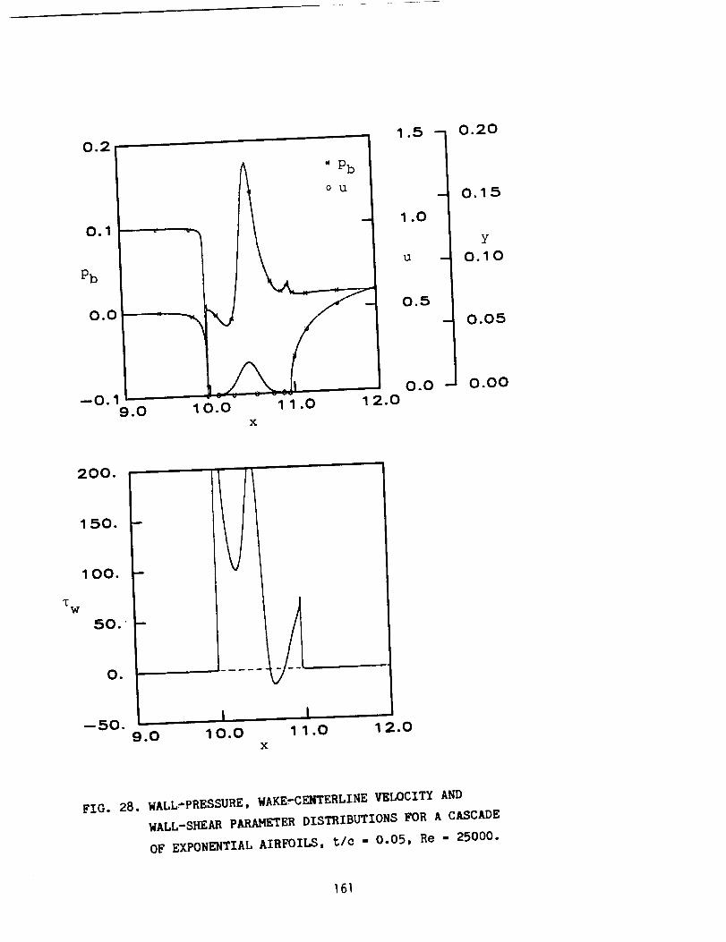
0.2
0.1
Pb
0.0
--0.19.0
1.5 "] 0.20
(_ " Pb
o u -I 0.15
' 1.0 |
| Y
u _ 0.10
1" --,, No o.o5
0.0 0.00
10.0 11.0 1 2.0X
200.
1,50.
100,
W
50.
O.
--50. L I I9.0 10.0 11.0 1 _,.0
X
FIG. 28. WALL_PRESSURE, WAKE.CEMTERLINE VELOCITY AND
WALL-SHEAR PARAMETER DISTRIBUTIONS FOR A CASCADE
OF EXPONENTIAL AIRFOILS, t/c = 0.05, Re = 25000.
161

a. CONFORMAL C-GRID (AFTER REF. 41)
b. 'LINE'PERIODIC' H'GRIDC. 'REGION'PERIODIC' H-GRID
FIG. 29. VARIOUS TYPES OF GRIDS FOR CASCADES.
162

. \.w _, _.._-V'-T', T---,_-l../" ,., \
_._ ,,'_"_/.J _ +-.__\._, _',_
a. OVERSET GRID
:ONE 4
PATCHBOUNDARY
PATCHBOUNDARIES
ZONE1
l ZONE5ZONE3
ZONE2
PATCHBOUNDARY
Ii iI!1 ,
ti ,
'; ! i
I
-, ]]- ' ! J _1
I I ---
I I i --_
''It
' ///a
• _ _ _ / / _/ / ,i it,
I I
I
b. PATCHED-DISJOINT GRID o- PATCHED-JOINT GRID
FIG. 30. TYPES OF MULTI-BLOCK STRUCTURED GRIDS.
163

/
0
i-i f._0
m: Z
r._oo=
o_
164

---E)
i
-'t,,)
F--1I
LIr,.9 ,_ :
L9
--E}
L9
I --u=rj
0
oI-t
I
:iL C._
u
n_
165

/
/
\_-Interface
a. CELL WITH NON-STANDARD NUMBER OF FACES
boPOINT WITH NON-STANDARD NUMBER OF NEIGHBOURS
FIG. 33. TYPES OF SPECIAL CELLS AND POINTS.
166

K
L
c1
81
E' D1_,,//_/////z.,_/z,_/
E II
G
B"
G' D
C
H
F1
FIG. 3_. 3-D VIEW OF THE COMPUTATIONAL DOMAIN.
167
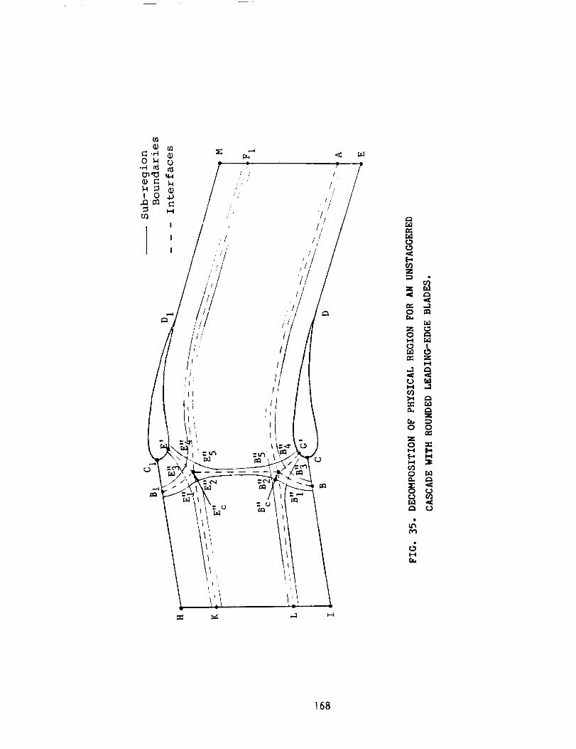
I
I
8
Z
_ Z
0 0
Z0
f.-, I-I
c_0 r.'l
Hf.l.,
168

m_
+
i
+
i
ic.D
i
4.-
1I
II
li
I--I
4-
ID
4-
I
L)
m_r.'1r.'l
r._
£..,I--I
H,--I
I--I
I
H
0
m_
Fa_
0
= d
.P. ,.
Z _
169
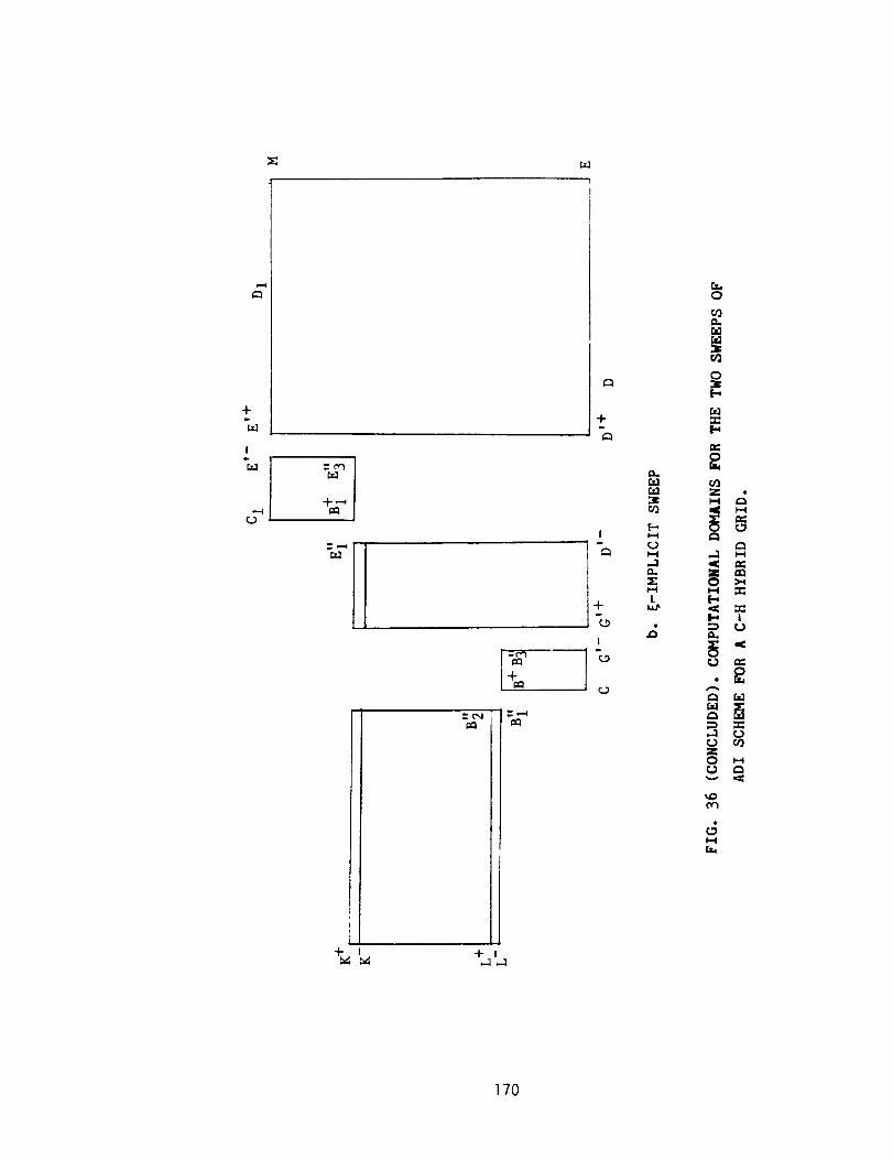
+D
r._
I
i-I-
.-c,.i
+t-I _-1
÷
I
+D
I
r_
E-,I--I
I-I--1
I-4
L
r_0
r._D.,r_
r._:z:
c/'j
V. =
,=_ c..)
Z0
I.=4
170
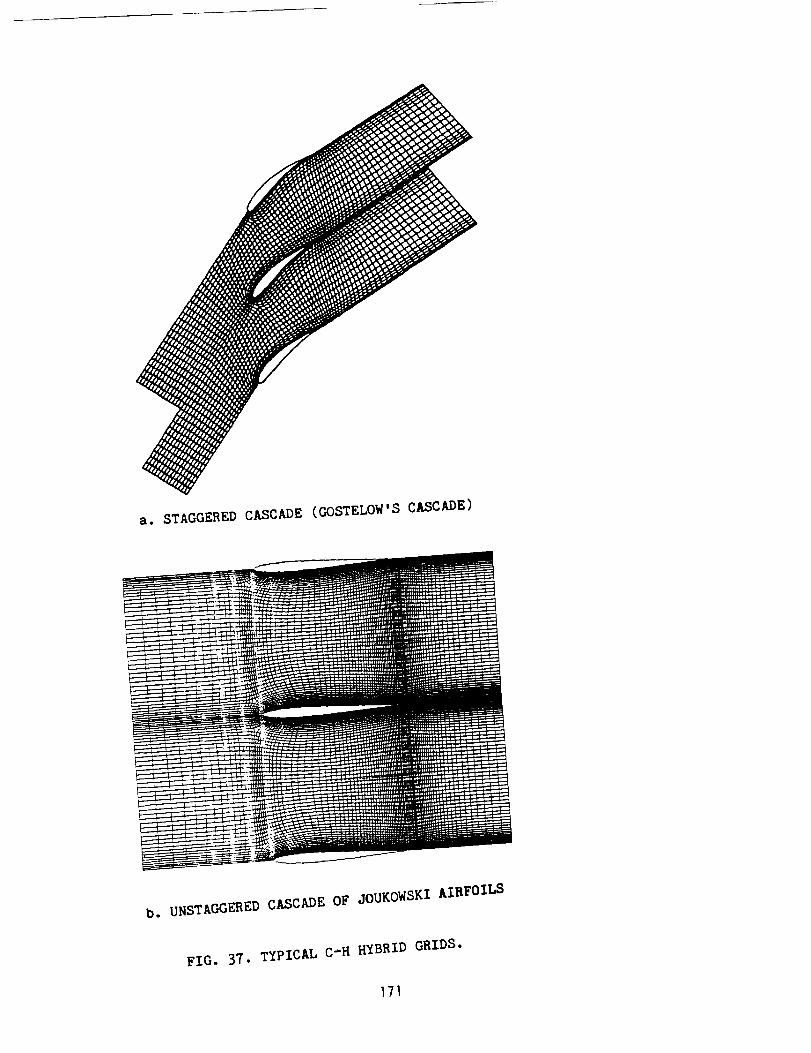
a. STAGGERED CASCADE (GOSTELOW'S CASCADE)
b. UNSTAGGERED CASCADE OF JOUKOWSKI AIRFOILS
FIG. 37. TYPICAL C-H HYBRID GRIDS.
171

aJ
/-4CI
-<-.
At
a. TWO-STEPS OF THE SOLUTION
PROCEDURE
bl b. ENLARGED VIEW OF LE REGIONS
FIG. 38. MARCHING DIRECTIONS FOR SEMI'ELLIPTIC FLOW-
SOLUTION PROCEDURE ON C=H HYBRID GRID.
172

0.8 1.5 - 0.20
U
0.15
y
0.10
0.05
0.0 - 0.00
a. SURFACE PRESSURE AND WAKE-CENTERLINE VELOCITY DISTRIBUTIONS
50.
40. --
_0. -
20. -
10. -
O.
-1o. :--4.0
t I5.0 x 6.0 7.0
b. WALL-SHEAR PARAMETER DISTRIBUTION
FIG. 39. RESULTS FOR A CASCADE OF JOUKOWSKI AIRFOILS
USING C-H HYBRID GRID, Re - 150.
173
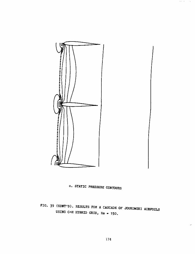
C. STATIC PRESSURE CONTOURs
FIG. 39 (CONTtD). RESULTS FOR A CASCADE OF JOUKOWSKI AIRFOILS
USING C_H HYBRID GRID, Re - 150.
174
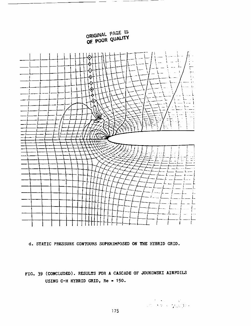
oRIGINAL pAGE |SOF poOR QUALfP(
d. STATIC PRESSURE CONTOURS SUPERIMPOSED ON THE HYBRID GRID.
FIG. 39 (CONCLUDED). RESULTS FOR A CASCADE OF JOUKOWSKI AIRFOILS
USING C-H HYBRID GRID, Re - 150.
175

0.8
0.4
Pb
0.0
--0.4- -
--0.8_4-.0
0 u
5.0 x 6.0 7.0
1 .5 - 0.20
u
0.15
0.05
0.0 - 0.00
a. SURFACE PRESSURE AND WAKE-CENTERLINE VELOCITY DISTRIBUTIONS
100.
"1" W
80.
60.
4-0.
20.
O.
1 I--20.4.0 5.0 × 6.0 7.0
b. WALL_SHEAR PARAMETER DISTRIBUTION
FIG. 40. RESULTS FOR A CASCADE OF JOUKOWSKI AIRFOILS
USING C'H HYBRID GRID, Re - 600.
176
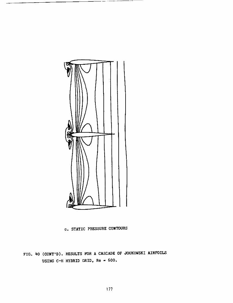
C. STATIC PRESSURE CONTOURS
FIG. 40 (CONT'D). RESULTS FOR A CASCADE OF JOUKOWSKI AIRFOILS
USING C-H HYBRID GRID, Re - 600.
177
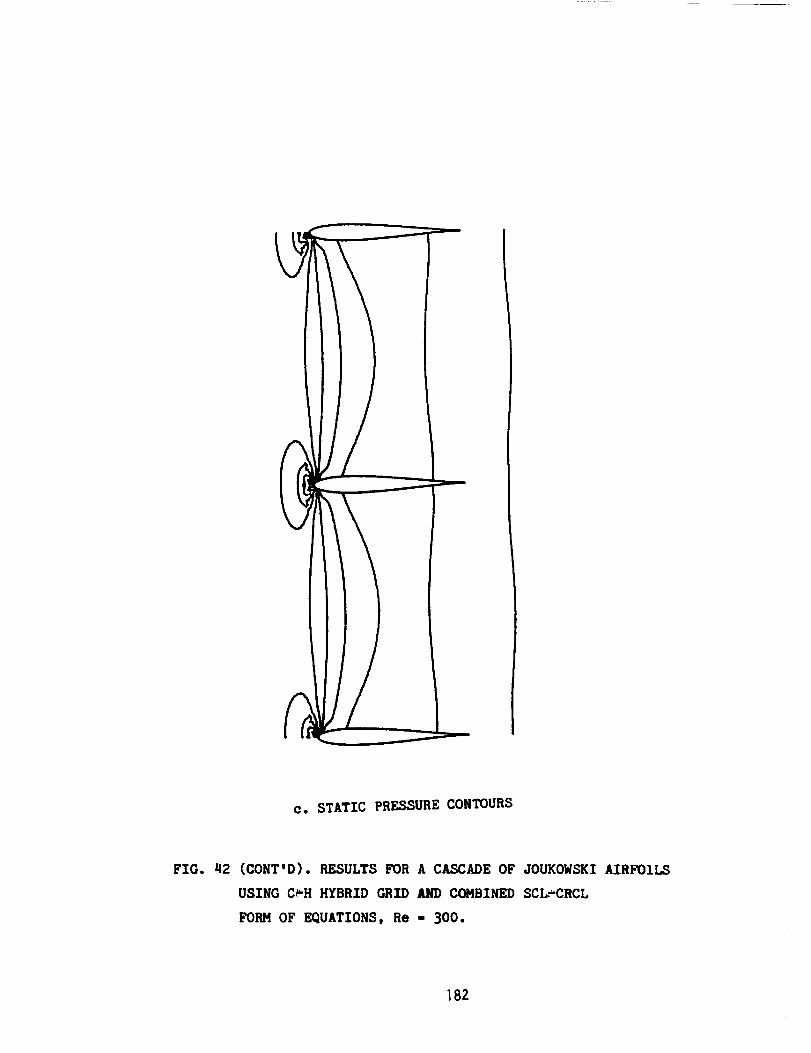
C. STATIC PRESSURE CONTOURS
FIG. 42 (CONT'D). RESULTS FOR A CASCADE OF JOUKOWSKI AIRFOILS
USING C_H HYBRID GRID AND COMBINED SCL-CRCL
FORM OF EQUATIONS, Re - 300.
182

¸ I
J
I I
-_# _
-i \T_'- -L
+----4 _
I
J
d. STATIC PRESSURE CONTOURS SUPERIMPOSED ON THE HYBRID GRID.
FIG. 42 (CONCLUDED). RESULTS FOR A CASCADE OF JOUKOWSKI AIRFOILS
USING C_H HYBRID GRID AND COMBINED SCL'CRCL
FORM OF EQUATIONS, Re - 300.
]83

Report Documentation PageSpice Mmtn,s_fmt_)n
1. Report No. 2. Government Accession No. 3. Recipient's Catalog No,
NASA CR- 4180
4. Title and Subtitle
Simulation of Two-D1menslonal Vlscous Flow Through
Cascades Uslng a Seml-E111ptlc Analysis and
Hybrld C-H Grlds
7. Author(s)
R. Ramamurtl, U. Ghla, and K.N. Ghla
9. Pedorming Orgenization Name and AddressUniversity of Cincinnati
Dept. of Aerospace Englneerlng and Engineering Mechanics
and Dept. of Mechanlcal and Industrial EnglneerlngC1ncinnatl, Ohlo 44221
12, SponsoringAgency Name and Address
National Aeronautlcs and Space AdmlnIstratlon
Lewls Research Center
Cleveland, Ohlo 44135-3191
5. Repod Oate
October 1988
6. Performing Organization Code
8. Pedorming Organization Report No.
86-9-71 (E-4286)
10. Work Unit No,
505-62-21
11. Contract or Grant No.
NAG3-194
13. Type of Report end Period Covered
Contractor ReportFinal
14. Sponsoring Agency Code
15. Sup_ementa_ Not_
Project Manager, Peter M. Sockol,Research Center.
Internal F1uld Mechanics Division, NASA Lewl s
16. AbstractA semi-elliptic formulation, termed the interacting parabolized Navier-Stokes (IPNS) formulation, is
developed for the analysis of a class of subsonic viscous flows for which streamwise diffusion is neg-
ligible but which are significantly influenced by upstream interactions. The IPNS equations are
obtained from the Navier-Stokes equations by dropping the streamwise viscous-diffusion terms butretaining upstream influence via the streamwise pressure-gradlent, A two-step alternating-direction-explicit numerical scheme is developed to solve these equations. The quasi-linearization and discre-
tization of the equations are carefully examined so that no artificial viscosity is added externally
to the scheme. Also, solutions to compressible as well as nearly incompressible flows are obtained
without any modification either in the analysis or in the solution procedure. The procedure isapplied to constricted channels and cascade passages formed by airfoils of various shapes. These
geometries are represented using numerically generated general curvilinear boundary-oriented coordi-
nates forming an H-grid. Stagnation pressure, stagnation temperature and streamline slope are pre-
scribed at inflow, while static pressure is prescribed at the outflow boundary. Results are obtained
for various values of Reynolds number, thickness ratio and Math number. The regular behavior of the
solutions demonstrates that the technique is viable for flows with strong interactions, arising due toeither boundary-layer separation or the presence of sharp leading/trailing edges. Mesh refinement
studies are conducted to verify the accuracy of the results obtained. A new hybrid C-H grid, more
appropriate for cascades of airfoils with rounded leading edges, is also developed. Appropriatedecomposition of the physical domain leads to a multi-block computational domain bounded only by thephysical-problem boundaries. This permits development of a composite solution procedure which, unlikemost found in literature, is not a patching procedure. Satisfactory results are obtained for flows
through cascades of 3oukowski airfoils. The implementation of the IPNS formulation on the C-H grid
exposes two _mall portions of the grid interfaces and these require special treatment. However, with
a hybrid grid, the use of complete Navier-Stokes equations is recommended, so as also to avoid incon-
sistencies in the parabolization approximation due to changing orientation of the coordinates at agiven location.
17. Key Words (Suggested by Author(s)}
Parabolized Navier-Stokes; Cascades; Channels; Compositegrids; Parabolized Navier-Stokes equations with upstreaminteraction via pressure; Alternating-dfrection explicinumerical method; General nonorthogonal grids; Compositeprocedure for hybrid grids; Cascades and channels; Com-pressible and incompressible flow; Separated flows
19. Security Cle_it. (of thie report) 120. Security Cleludf, {of this page)
Unc I as sIf ted I IJncl as s t f tedNASA FORM 1621_ OCT 8S
18. Distd_tion S_tement
UnclasslFled- Unlimited
Subject Category 02
21. No of pages 122 Price"
196 1 A09
"For sale by the National Technical Information Service, Springfield, Virginia 22161
NASA-Langley, 1988


![search.jsp?R=19900004927 2020-03-25T03:25:35+00:00Z I 1 ... · COLLEGE OF ENGINEERING AND TECHNOLOGY OLD DOMINION UNIVERSTTY NORFOLK, VIRGINIA, ... [10,11]. There, the coplanar and](https://img.pdfslide.us/doc/110x75/5ea2684fe3174e3e7a3c6760/r19900004927-2020-03-25t0325350000z-i-1-college-of-engineering-and-technology.jpg)