E XTENDED F AST S EARCH C LUSTERING A LGORITHM : W IDELY D ENSITY C LUSTERS , N O D ENSITY P EAKS

Jan Zizka et al. (Eds) : DBDM, CICS, CCNET, CSIP - 2015

pp. 01–17, 2015. © CS & IT-CSCP 2015 DOI : 10.5121/csit.2015.50701

EXTENDED FAST SEARCH CLUSTERING

ALGORITHM: WIDELY DENSITY

CLUSTERS, NO DENSITY PEAKS

Zhang WenKai

1 and Li Jing

2

1,2School of Computer Science and Technology, University of Science and

Technology of China, Hefei, 230026, China [email protected]

[email protected]

ABSTRACT

CFSFDP (clustering by fast search and find of density peaks) is recently developed density-

based clustering algorithm. Compared to DBSCAN, it needs less parameters and is

computationally cheap for its non-iteration. Alex. at al have demonstrated its power by many

applications. However, CFSFDP performs not well when there are more than one density peak

for one cluster, what we name as "no density peaks". In this paper, inspired by the idea of a

hierarchical clustering algorithm CHAMELEON, we propose an extension of CFSFDP,

E_CFSFDP, to adapt more applications. In particular, we take use of original CFSFDP to

generating initial clusters first, then merge the sub clusters in the second phase. We have

conducted the algorithm to several data sets, of which, there are "no density peaks". Experiment

results show that our approach outperforms the original one due to it breaks through the strict

claim of data sets.

KEYWORDS

Clustering, Density, Density peaks, K-nearest neighbour graph, Closeness &Inter-connectivity

1. INTRODUCTION

Clustering is known as the unsupervised classification in pattern recognition, or nonparametric

density estimation in statistics[1]. The aim is to partition given data set of points or objects into

natural grouping(s) according to their similarity to improve understanding on the condition of no

priori-knowledge, or be as a method to compress data. Cluster analysis has been widely used in a

lot of fields, like computer version ([2], [3], [4]), bioinformatics ([5], [6], [7]), image progressing

([8], [9], [10], [11]), Knowledge Discovery in Databases(KDD), and many other areas ([12]).

Thousands of clustering algorithms have been proposed, challenges still remain: differing shapes,

high dimensions, how to determine the clusters number, how to define a right clustering, hard to

evaluate.

Density-based clustering algorithms which classify points by identifying regions heavily

populated with data, such as DBSCAN [13] and GDBSCAN [14], OPTICS [15], and DBCLASD

[16], have performed well while handling problems of arbitrary shapes of subclasses. DBSCAN

[13] is a representative of density-based methods, by the definition of core points, density

connection, in which clusters defined as high density regions separated by low density regions in

2 Computer Science & Information Technology (CS & IT)

the feature space can be detected without the need for clusters number. However the appropriate

threshold MinPts(minimum number of points) for distinguishing core points from border points is

hard to select, with a high MinPts, thin clusters(relative low density) would be ignored.

Similar to DBSCAN [13], recently, CFSFDP (clustering by fast search and find of density peaks)

[17] was proposed by Alex and Anlessandro to detect non-spherical groups, which does not need

to pre-specify the number of clusters of variant shapes either. In addition, CFSFDP needs less

parameters. CFSFDP finds the clusters of points by a two phase progression. During the first

phase, CFSFDP uses a well-designed decision group to find out the cluster centres, so-called

density peaks. During the second phase, each remaining point is assigned to the same cluster as

its nearest neighbour of higher density. In a DBSCANs perspective, CFSFDP assumes that every

object is density-connected with its nearest neighbour of higher density. Compared to mean-shift

methods such as[18], [19], CFSFDP [17] is computationally cheaper for the procedure of

maximizing the density field for each data point in the mean-shift approach. By the experiments

of identifying the number of subjects in the Olivetti Face Database [20], the team have shown

CFSFDP’s capacity to solve high dimensional data [17].

However, in our opinion, there are some drawbacks of the beautiful CFSFDP [17], which will

limit the application of CFSFDP. Firstly, just as DBSCAN [13], thin clusters would not be

captured by the decision graph. Besides, a rigid hidden requirement for getting right clusters is

that, each cluster in the data sets must have a density peak and only one peak is promised,

otherwise CFSFDP will split natural groups. In this paper, inspired by CHAMELEON [21], we

present a novel hierarchical clustering algorithm based on CFSFDP. Thus our approach can find

thin clusters. In addition, it eliminates he strict claim of density peaks. To display our efforts, we

benchmark our algorithm on the data sets draw from [21],[22], [23], of which there is no unique

density peak for each cluster. Our technique gets partitions of these data sets as well as that

generated by the methods proposed in the papers where the data set was designed.

We discuss details of CFSFDP [17], CHAMELEON [21] in Section 2. In Section 3, we present

drawbacks of CFSFDP and our efforts to overcome these limitations. Section 4 describes our

algorithm in detail. In Section 5, we benchmark the performance of our approach on some data

sets from other literatures. Finally, a conclusion and direction of future worksare shown in

Section 6.

2. BASIC CONCEPTS

This Section presents two methods and some concepts involved in our technique, what are

necessary to understand our approach. If one has been familiar to CFSFDP and CHAMELEON,

he could skip to Section 3, where we discuss some disadvantages of CFSFDP in details.

2.1. CFSFDP

CFSFDP [17] generates clusters by assigning data points to the same cluster as its nearest

neighbour with higher density after cluster centres are selected by users. The cluster centres are

defined as local density maxima, Alex and Alessandro designed a heuristic method for customers

to select the genuine cluster centres, what is named as decision graph.

Two important quantities are considered in the decision group: local density �� of each point,its

distance � frompoints of higher density. Definition of �� , � follows:

Definition 1: The density of a point , denoted by ��, is defined as

Computer Science & Information Technology (CS & IT) 3

�� = ∑ (�� − ��)� .(1)

Where χ(x) = 1 if x < 0 and χ(x) = 0 otherwise, and �� is a cutoff distance, which is the only

parameter need to be determined by customers. In principle, �� equals to the number of points

which are closer than �� to point .

Definition 1: The minimum distance of point from anyother point of higher density, denoted by

�, is computed by

� = min�:�� . (2)

Figure1. The CFSFDP in two dimensions. (1) Point distribution. Data points are ranked in order

of decreasing density. (2) Decision graph for the data in(1). Different colors correspond to

different clusters. [17]

Notice that, for the point of largest density, � is redefinedas � = max�∈!"#"$%# �� . The simple

observation that points ofhigh local density and high density distance are local density maxima,

namely density peaks or cluster centres, is the core of this procedure to select cluster centres.

To identify density peaks defined as below, a method named as ”decision graph” is introduced to

help users to make a decision. Basically, decision graph is a figure plotting �as afunction of �� , is illustrated by the two-dimensional simpleexample in Fig.1. Points 1 and 10 are the only two

points ofhigh δ and high ρ, as a result, they are the cluster centres. Points 26, 27, 28 can be

considered as outliers for a relatively high δ and low ρ (which indicates that they are isolated

points).

After cluster centres have been found, CFSFDP allocates the rest points to the same cluster as its

nearest neighbourhood with higher density.


2.2. CHAMELEON

CHAMELEON discovers clusters of a given data sets gradually by finding groups consisted of

most similar points. There are 3 main steps in CHAMELEON: create the k-nearest Neighbour

Graph according to data points, partition the graph into sub-classes, then merge the subsets. It’s

common to model data items as a graph in agglomerative hierarchical clustering techniques[1],

CHAMELEON models data based on the widely used k-nearest neighbour graph technique. After

the graph was built, a efficient graph partitioning algorithm mMETIS[24]is used to find the initial

sub-clusters. As criteria to aggregate the sub clusters, CHAMELEON computes the relative

interconnectivityRI(+� , +�)and relative closeness RC(+� , +�) between each pair of clusters +� and

+� . In the merge phase,each round the cluster pair of highest

RI(+�, +�) × /+(+�, +�)0 (3)

will be merged, where β is a user defined parameter to give different importance to the two

criterions. The merge progress will be stop when cluster number is equal to the number

predefined or there is no cluster pair of which the value of (3) is bigger than user determined

threshold.

In (3), the relative inter-connectivity RI(+� , +�)betweencluster +� and cluster+� is defined as the

sum of the weight of edges span the two clusters normalized with respect to the internal inter-

connectivity of cluster +� and cluster +� . Theinternal inter-connectivity of cluster is computed by

addingthe weight of edges that partition the cluster into two roughly equal parts. Meanwhile

CHAMELEON defines the relative closeness RC(+� , +�) of cluster +� and cluster +� as theaverage

weight of edges span the two clusters, which alsois normalized with respect to the internal

closeness of each cluster.

Figure 2. Clustering considering either closeness or inter-connectivity. [21]

The key difference of CHAMELEON and other hierarchical clustering algorithms like CURE

[25], ROCK [26] is that it accounts for both inter-connectivity and closeness while identifying the

most similar pair of clusters in the third step[21]. The disadvantages of only considering either

closeness or inter-connectivity is these schemes could merge wrong pair of clusters. A sample of

that was given by George, as shown inFig.2. In Fig.2.(1), algorithms only based on closeness

(CURE and related schemes) merge incorrectly because through clusters of (a) — the dark-blue

and green clusters — are closer to each other than the case of (b) — the red and cyan clusters,

clusters of (b) connect better than those of (a). In Fig.2.(2), the inter-connectivity of the dark-blue


cluster and the red cluster is bigger than that of the dark-blue cluster and the green cluster,

however the dark-blue cluster is closer to the red cluster than the green one. Thus an algorithm

based only on the interconnectivity(ROCK [26]) merge the dark-blue cluster with the red cluster

incorrectly.

3. LIMITATIONS OF CFSFDP AND OUR CONTRIBUTION

In this Section, firstly we discuss our understanding towards limitations of CFSFDP in theory. To

help illustrate the limitation intuitively, an instance is presented.

CFSFDP has got high performance classifying several datasets, the success of these examples

verifies the availability of CFSFDP in some degree. As shown in Section 2, it generates groups by

identifying clusters with density maxima. However, it is impossible to get natural clusters by

CFSFDP when the local densities of data points in some or all natural clusters of the data sets is

random distributed, such that instead of one density peak two or more density peaks appear in one

cluster. In such a case, it is hard for CFSFDP to pick up all the reasonable cluster centres. What’s

more, even if a reasonable cluster centre set is found by CFSFDP, the natural cluster would be

split. Reasonable cluster centre here means that a point as density maximal, with which, the result

cluster of CFSFDP clustering procedure (assign each point to the same cluster of its nearest

neighbour of higher density than itself) is not consisted of parts of different natural clusters.

Reasonable cluster centre set means a set of reasonable cluster centres. The cluster centre set

presented in Fig.4.B, is an unreasonable cluster centre set for the red cluster is composed of part

of the “arc” cluster and part of left cluster.

Figure 3. The data set drawn from [22]. There are 3 native clusters of diversedensity, complex shapes, two

of the three are surrounded by the third one.

Figure 4. CFSFDP groups the data set in Fig.3, Different colors correspond to different clusters,

the figure above in each sub figure is the decision graph, the figure below is the correspond

dividing result. (1)�� = 1:101 such that the largest density equals to about 1% of the number of

points size, 2 clusters.(2)�� = 1:540 such that the largest density is equal to about 2% of the size

of data set, 2 clusters. (3)�� = 2:250, such that the largest density equals toabout 4% of the

number of total points, 5 clusters. (4)�� = 3:814, such that the largest density equals to about 10%

of the number of total objects, 3 clusters.


Let’s consider the test case in Fig.3. The data set is drawn from [22], there are 3 natural clusters

in the data set: the left cluster surrounded by the arc, the right cluster surrounded by the arc, and

the arc cluster. We test CFSFDP on this data set by variant dc, the clustering result of some

values(1.101, 1.540, 2.250, 3.814) is shown in Fig.4. Except the experiments presented in Fig.4,

many other values of dc have been tested, unfortunately CFSFDP can’t divide the points into

natural groups with any value of ��. In particular, CFSFDP makes mistake on the arc cluster,

parts of which are resigned into wrong clusters.

Firstly, poor ability of decision graph to select cluster centres is one reason of such a bad

outcome, because performance of CFSFDP is highly sensitive to the procedure determining

cluster centres [17] says, cluster centres of relative high local density ρ & relative high δ are of

remarkable location in the decision graph, and indeed its true for some cases, as shown in Fig.1

where cluster centres are of high ρ and high δ in global. Nevertheless, when clusters of more

complex data sets, either thin cluster centres of relative low ρ and high δ, or other cluster centres

of relative high ρ and low δ, would be overlooked easily. As an example, in Fig.4, the relative

thin cluster centres belong to the “arc” cluster are easily ignored for we only select the points of

remarkable location as cluster centres. One may argue that with a more suitable value

of��,density peaks would be prominent in decision graph and be easy to point out by users. In our

opinion, it may be or may not be, it depends on the data sets. A good method to select cluster

centres should reduce its dependency upon data sets as much as it can, such that it would detect

diverse density or diverse δ cluster centres.

Another cause of wrong clusters detected by CFSFDP is that CFSFDP divides points based on

cluster centres, such that CFSFDP might divide the natural cluster if there are more than one

cluster centres was determined in a natural cluster. For example, Fig.4 shows the clustering

consequence of the[22] data set after choosing reasonable cluster c centre set by our new decision

graph. In Fig.4, points of the arc cluster which is split into several clusters. Inspired by the

clustering progress of hierarchical clustering algorithm, a novel clustering algorithm consisted of

two phases brings out to us: 1) generate subclasses by CFSFDP, 2) merge the sub classes by the

similarity between clusters.

3.1. Modelling the Similarity between Clusters

To break through the barriers of agglomerative hierarchical approaches discussed in Section 2,

our algorithm looks at their Relative Inter-connectivityRI(+�, +�) and their Relativecloseness

RC(+�, +�) while merging cluster +� and cluster +� , which is similar with the aggregation phase of

CHAMELEON. By considering both of these criteria, ourscheme selects clusters that are well

connected as well asclose together to merge. However, there is a shortage inCHAMELEON that

is CHAMELEON, which models sub clusters based on the widely used k-nearest neighbour

graph, would fail to merge the correct cluster pair in some cases. To solve that, we using a variant

of k-nearest neighbour graph to model the sub clusters. Other than the difference of the model to

represent sub clusters, we compute the relative inter-connectivity and the closeness almost the

same as CHAMELEON, we also use the value defined by (3) to model the similarity between

clusters.

In this Section, firstly we show the detail of the relative inter-connectivity and the relative

closeness. In the remainder, the detail of drawback in CHAMELEON’s merging phase is

presented, then our solution is followed.

The relative inter-connectivity RI(+� , +�) between cluster +� and cluster +� is given by


RI1+�, +�2 =34567,689

:;�::;�:<=;�=

3467>=6�=

:;�:<=;�=34;�

. (4)

Where ?+@+,+AB = ∑ ?(C, D) is sum of weight of edgesconnecting the two clusters. E(u, v) is

defined as (4), this isthe main difference between CHAMELEONs merging phaseand our

merging phase.

The Relative closeness RC1+�, +�2is computed by

RC1+�, +�2 =GI̅;{;�,;�}

:;�::;�:<=;�=

G̅I;;�>

=6�=:;�:<=;�=

G̅I;;�

. (5)

Where L3̅4{;�,;�} =345;�,;�9|3(N,O)| is the average weightof edges span the two clusters. To get the value

of inner criteria, as ?+4�or L3̅4;�, CHAMELEON takes graph partitioningtechnology to bipartite

the target cluster, whilewe split the target cluster by CFSFDP. In particular, at first, we utilize the

CFSFDP clustering algorithm with the novel decision graph(described in previous part of this

Section) to clustering the points of current cluster into two sub classes; then we compute F based

on the clustering result. There are two advantages of taking use of CFSFDP rather than graph

partitioning methods to split the target cluster. Firstly, CFSFDP is very fast with specific cluster

centres, the time complexity isо(n), k is the number of points of the target cluster. The selection

of cluster centres can be done in constant time based on the computation in the initial clustering

phase. Secondly, we use CFSFDP in all phases of our clustering method to keep consistency in

theory, in our view, that meets the famous Ockham’s Razor principle.

CHAMELEON models the similarity based on the widely used k-nearest neighbour graph. The

benefit of representing data as a k-nearest neighbour graph covers that simplifying topology of

data sets by disconnecting the points are far apart, capturing the concept of neighbourhood

dynamically, and there are many methods offered to handle graph data [21].However, in the

merge phase, we find that CHAMELEON based on the standard k-nearest graph would fail to

merge the correct cluster pair in some cases. The example in Figure.5.(1)illustrates, an algorithm

that considering the inter-connectivity as CHAMELEON (presented in Section 2) will prefer to

merge in correctly the red cluster with the blue cluster, rather than with the green cluster. Notice

that, because the blue cluster is much sparser than the red cluster, as a result, the measure of

connectivity and closeness depends on point P, and almost all the k-nearest neighbours of point P

belong to the red cluster, leading to that both the criteria (inter-connectivity and closeness) of the

red cluster and the blue cluster are higher than those of the red cluster and the green cluster.

Figure 5. (1) Chameleon prefers to merge incorrectly the red cluster with theblue cluster rather with the

green cluster. (2) A simplified instance to explain why Chameleon fails in (1).


Further, we find that CHAMELEON fails because it is almost impossible for CHAMELEON

based on the standard k-nearest graph to distinguish case (a) from case (b) inFigure.5.(2).Where

the weight of edges is nearly the same. In figure.5, we ignoring the normalization because the

inner criteria are the same in this example.

To address that disadvantage, we bring out a variant of k-nearest neighbour graph to model the

sub clusters. In this paper, the edge connecting point of cluster+� with point of cluster+� is given

by

E(u, v) = max ( @?(C, P):C ∈ +� ∩ P ∈ +� ∩ C ∈ RS(P) ∩ P ∈ RS(C)B ). (6)

WhereE(u, v) represents the edge connecting point u with point v. KN(∙) is an operator to get the

k-nearest neighbor.The max (∙) function is to get the edge of maximum weight,the weight here

means the similarity. By only considering the edge of maximum weight, our approach can

distinguish the two type k-nearest neighbour relationship. In figure.5. (2). (b), we remove the two

slash edges, such that, we can get a smaller inter-connectivity of case (a) than that of case (b).

Even if there is still a similar closeness, it is possible to distinguish case (a) from case (b) by

giving a higher importance to the inter-connectivity, by specifying a value smaller than 1.o to β in

(3).

4. THE EXTENDED CFSFDP (E_CFSFDP)

Algorithm 1 E_CFSFDP (X, WX, YZ[\]^_à, β)

Inputs:

Χ= {bc,bd, ef, …, eZ} Set of data objects

WX : radius to computeρ.

YZ[\]^_à: value of neighbour number while modelling the cluster similarity.

β : parameter to control the importance of the two criterion (3).

Output:

C = {gc, gd, gf, …, gZ} Set of clusters

{Phase I} find initial sub-clusters by CFSFDP

1: compute the similarity matrix.

2: compute the local density ρ and the distance δ of each object.

3: select cluster centres by decision graph.

4: allocate each point to the same cluster as its nearest neighbour of higher ρ.

{Phase II} merge the sub-clusters

5: construct the model of sub-clusters.

6: compute thehi(g\, gj) × kg(g\, gj)l matrix for eachsub-clusters pair {g\, gj} based on

the model built in step4.

7: merge the cluster pair of highest hi(g\, gj) × kg(g\, gj)l.

8: repeat step 6 and step 7 until the termination conditions are meet.


4.1.The Description of E_CFSFDP

While CFSFDP algorithm needs one parameter �� , our algorithmE_CFSFDP requires three

parameters for the extensions presented in Section 3. As in CFSFDP, ��is a value to computethe

local density ρ in (1). [17] gives an empirical hint to specify��, choosing the value so that the

average number of neighbours is around 1% to 2% of the total number of points in the data set.

Sm%�nopqr is the number of neighbours for modelling the similarity of sub-clusters. β is the factor

to control the relative importance of inter-connectivity and closeness in the merge step.

We describe the steps of our algorithm E_CFSFDP in Algorithm 1.

Our algorithm starts at getting the similarity matrix of the data set. Many methods have been

proposed by the machine learning community to measure the similarity between different objects,

such as the common used Euclidean Distance, Mahalanobis Distance, Cosine Distance, SNN

Similarity. One can choose appropriate method based on the application, i.e., Euclidean Distance

for 2D data set, SNN Similarity for high dimensional data set. After that, we initialize the

clustering group by CFSFDP. What’s different from the standard CFSFDP, our scheme chooses

as more cluster centres as possible in step 3 to overcome the limitation of CFSFDP described in

Section 3.

In Phase II, the algorithm computes the value of necessary variables for merging in Step 5 and

Step 6. In Step 5,the variant k-nearest neighbour graph is constructed, where algorithms based on

k-d trees can be used [27]. In Step 7,E_CFSFDP combines two clusters into one in each iteration.

To do so, the RI(+� , +�) × /+(+� , +�)0matrix needs toupdate in each loop, and the renewal of

value refer to thesub cluster has been merged is necessary.

As a hierarchical algorithm, E_CFSFDP will not terminate until there is only one cluster

remained. However, in real application, that seems meaningless. So in real application,

E_CFSFDP usually terminates at the moment when the number of clusters is equal to the user

specified parameter k. And CHAMELEON [21] proposes an alternative scheme to terminate the

combination, that is to set two user input threshold stu,st4 , thus the algorithm stops when there is

no cluster pair, of which the inter-connectivity RI and the closeness RC are bigger than the

respond threshold stu and st4 . While in the experiments of this paper, we stop thealgorithm by a

value k of genuine clusters’ number.

4.2. Performance Analysis

The runtime complexity of E CFSFDP mainly depends on the two phases in the scheme. In the

initial phase, E_CFSFDP is almost the same as CFSFDP.

Let´s consider the runtime of CFSFDP. CFSFDP needsо(vw)to compute local density and the

distance where n is the number of objects in the input data set. For the progress to determine the

cluster centres, we take no account of the time for the user to select cluster centres due to that is

hard to quantize correctly. CFSFDP needsо(n)to construct thedecision graph. After the cluster

centers are chose, CFSFD Passigns each point to the same cluster as by the order of descend local

density, thus CFSFDP needsо(n log v) to sortthe points with quick sort [28], and CFSFDP’s

assignment procedure costsо(n), such that, the total time complexity of CFSFDP isо(vw) if the

similarity matrix has been finished. Inthe first phase, E_CFSFDP costs the same time as the

overall time of original CFSFDP, indicates the time complexity of E_CFSFDP’s first phase

isо(vw). Moreover, our analysis will focus on the computation of inter-connectivity and relative

closeness which have been described in Section 3, for the main cost of E_CFSFDP’s second

phase comes from the computation and the update of these criteria.


The computation of the two criteria is based on the variant-nearest neighbour graph, which can be

constructed based on the basic k-nearest neighbour graph. For low dimensional dataset, the

amount of time to construct the basic k-nearest neighbour graph is о(n log v) if algorithms based

on k-d trees [27] areused. For high dimensional data set, schemes based on k-d trees are not

applicable ([29], [30]), leading to an overall time complexity ofо(vw). To get the variant model

presented in Section 3, our algorithm need to check all k nearest neighbours for each item, leading

to the runtime complexity isо(kn), k is the number of neighbours.

To simplify the analysis, we assume that each cluster is of the same size, thus if the number of

sub clusters is m, the size of each cluster is| v⁄ . E_CFSFDP needs to traverse part of the variant

k-nearest neighbour graph to compute the interconnectivity and relative closeness for each cluster

pair, of which data points belong to the cluster pair, resulting in time complexity ofо(2 v |⁄ ).

The amount of time of normalizing the inter-connectivity or the closeness is alsoо(2 v |⁄ ) for

thebisection costs the same time as that of CFSFDP’s alignmentprogress. In Step 5, there are

1�w2 cluster pairs to be solved,causing the amount of timeо(0.5vw × 2 v |⁄ ) =о(mn) .

Whilemerging iteratively, the runtime depends on the time of findingthe most similar cluster pair

and updating the criteria. By usinga heap-based priority queue, the amount of time required tofind

the most similar cluster pair isо(|w log |). The timeto update the matrix isо(n) for there are

most m − 1 steps,each step requires the time ofо(2 v |⁄ ).

Thus, the overall complexity of the extended CFSFDP(E_CFSFDP) isо(nw + v log v + |v).

Comparedto the runtime of original CFSFDPо(vw), the largest term nwof the two approaches

both comes from the computation oflocal density, the amount of time of our algorithm doesn’t

increase much, especially for a large value of n.

5. EXPERIMENTS

In order to demonstrate the performance of our algorithm E_CFSFDP, we benchmark it on

several 2D data sets consist of clusters of diverse density, shapes, which have not no unique

density peak for each cluster. The reason why we adopt 2D data sets to benchmark our scheme is

that it is easy to visualize the clustering results of 2D data sets, making the comparison of

different algorithms much easier. Our experimental study focuses on the comparison of the basic

CFSFDP and its extension E_CFSFDP proposed by us, to testify that E_CFSFDP can handle the

data set, in which there is no unique density peak for each cluster.

This paper measures the similarity between data points with the famous Euclidean Distance,

which is used widely to measure the similarity of spatial data, 2D or 3D. And though we

determine parameters ( �� , Sm%�nopqr , β) based onthe application, we will show that our

algorithm E_CFSFDP is robust with respect to parameters by presenting the clustering results of

E_CFSFDP with different combinations of value of �� , Sm%�nopqr , and β. Besides, for

convenience, we use percentage to denote the value of parameter �� , which is used in (1) to

compute the local density, i.e., we say �� = 2%,indicates that with the ��, s.t.,max � = 2% ×��(��).


Figure 6. 2D data sets to benchmark E_CFSFDP

5.1. Data Sets

Four data sets proposed by other papers are used to evaluate our algorithm in this paper. In

particular, Jain’s dataset is taken from [23], Chang’s dataset is taken from [22], Chameleon_1and

Chameleon_2 are drawn from [21]. As presented in Fig.6,clusters of the 4 data sets are of diverse

density, complex shapes. The most important feature of these data sets shared is no obvious single

density peak for most clusters, even in Chang’s data set, there is one cluster — the arc one —

which don’t have a unique density peak. We will show you that our algorithm performs better to

deal with this case below.

5.2. The Evaluation of Clustering Results

2.6.1. Jain’s data set

As shown in Fig. 6, there are 2clusters, 373 data points in the data set, one of the clusters is

denser than another. In this case, our approach E_CFSFDP expenses more time to be more robust

respect to parameter��. Fig.7 presents a lot of clusters found by CFSFDP with different �� and

selections of cluster centers. For CFSFDP’s performance is depended on the selection of density

peaks, we not only present the clustering result, but also show the decision graph and the

selections of cluster centers. As shown, CFSFDP gets perfect result when �� = {40%, 45%},

however it fails with other values, as �� = {1%, 2%, 10%}. By more experiments, we find

CFSFDP also divides Jain’s data set correctly with �� = {44%, 46%, 47%}.

As an extension of CFSFDP, our scheme not only can find genuine clusters with the same ��

whereas CFSFDP succeeds (E_CFSFDP can just specify the number of sub-clusters to be 2),but

also works fine whereas CFSFDP fails to perform well. E_CFSFDP finds the 2 natural clusters in

above data set with parameters of any combination of�� = {4%, 5%, 6%},Sm%�nopqr = {5, 10,

15}, β = {1, 2, 3, 4, 5}. To present the clustering progress better, we present the initial clusters

found by E_CFSFDP in Fig. 8. (2), (3), (4).


Figure 7. Clusters found in Jain’s data set by CFSFDP with different dc. Different colours correspond to

different clusters, there is no any relationship of colours in different figures.


Figure 8. Clusters found by E CFSFDP in Jain’s data set. (1) shows the final results of E CFSFDP. (2), (3),

(4) show the initial clusters.

2.6.2. Chang’s data set

There are 3 natural clusters in the data set, some clustering solutions proposed by CFSFDP have

been given in Fig. 4. We also conduct E_CFSFDP on this data set, the result is presented in Fig.

9. In the experiment, we have test CFSFDP and E_CFSFDP on this data set with many

parameters, the best result of each approach is given. In this case, E_CFSFDP is the obvious

winner.

Figure 9. Clustering results for Chang’s data set. (1) The original data set; (2)CFSFDP clustering result; (3)

E CFSFDP clustering result.

Notice that, on this data set, the clustering result of E_CFSFDP is 100% correct, as shown in Fig.

9. (3). That doesn’t mean E_CFSFDP is perfect, because in fact, with other values of ��, some

points between different clusters will be assigned to wrong cluster.


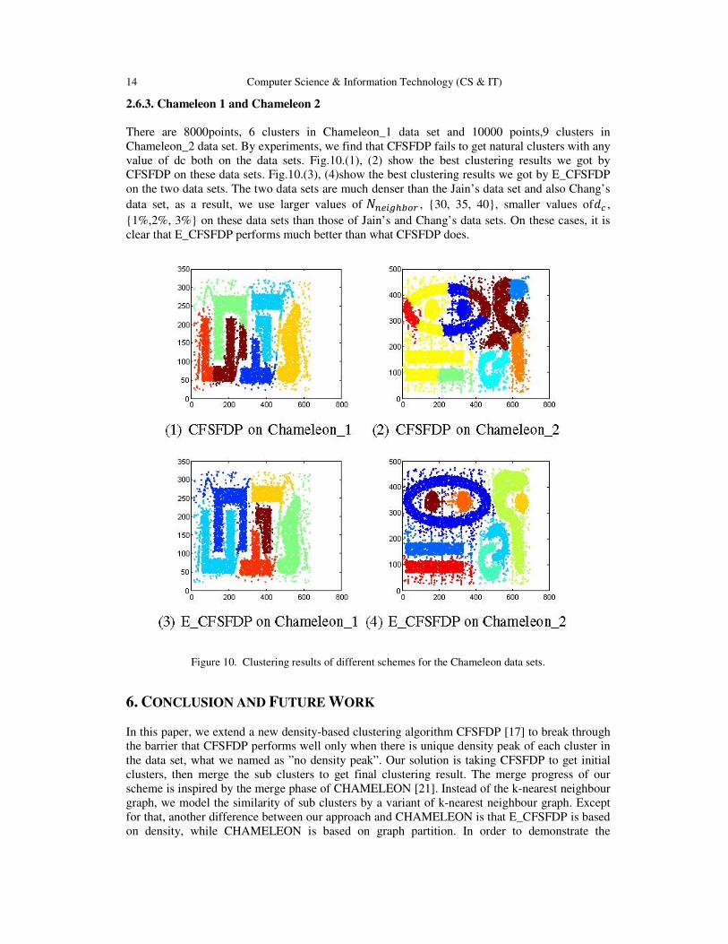
2.6.3. Chameleon 1 and Chameleon 2

There are 8000points, 6 clusters in Chameleon_1 data set and 10000 points,9 clusters in

Chameleon_2 data set. By experiments, we find that CFSFDP fails to get natural clusters with any

value of dc both on the data sets. Fig.10.(1), (2) show the best clustering results we got by

CFSFDP on these data sets. Fig.10.(3), (4)show the best clustering results we got by E_CFSFDP

on the two data sets. The two data sets are much denser than the Jain’s data set and also Chang’s

data set, as a result, we use larger values of Sm%�nopqr , {30, 35, 40}, smaller values of�� ,

{1%,2%, 3%} on these data sets than those of Jain’s and Chang’s data sets. On these cases, it is

clear that E_CFSFDP performs much better than what CFSFDP does.

Figure 10. Clustering results of different schemes for the Chameleon data sets.

6. CONCLUSION AND FUTURE WORK

In this paper, we extend a new density-based clustering algorithm CFSFDP [17] to break through

the barrier that CFSFDP performs well only when there is unique density peak of each cluster in

the data set, what we named as ”no density peak”. Our solution is taking CFSFDP to get initial

clusters, then merge the sub clusters to get final clustering result. The merge progress of our

scheme is inspired by the merge phase of CHAMELEON [21]. Instead of the k-nearest neighbour

graph, we model the similarity of sub clusters by a variant of k-nearest neighbour graph. Except

for that, another difference between our approach and CHAMELEON is that E_CFSFDP is based

on density, while CHAMELEON is based on graph partition. In order to demonstrate the


applicability of our algorithm to solve the case ”no density peak”, we conduct CFSFDP and

E_CFSFDP on several 2D data sets, there is no density peak for clusters of which. Although our

method doesn’t increase much more run time complexity than the original algorithm, it’s true our

algorithm spends more time than the original one.

In future studies, we will focus on reducing the run time of E_CFSFDP. What’s more, we will

apply it to high dimensional data sets. Another interesting direction is running it in parallel.

ACKNOWLEDGEMENTS

This work was supported by Key Technologies Research and Development Program of China

(No.2012BAH17B03),and the Chinese Academy of Science (No. 2014HSSA09).

REFERENCES [1] P. Berkhin, “A survey of clustering data mining techniques,” in GroupingMultidimensional Data, J.

Kogan, C. Nicholas, and M. Teboulle, Eds.Springer Berlin Heidelberg, 2006, pp. 25–71.

[2] H. Frigui and R. Krishnapuram, “A robust competitive clustering algorithmwith applications in

computer vision,” Pattern Analysis andMachine Intelligence, IEEE Transactions on, vol. 21, no. 5, pp.

450–465, May 1999.

[3] R. Achanta, A. Shaji, K. Smith, A. Lucchi, P. Fua, and S. Su?sstrunk,“Slic superpixels compared to

state-of-the-art superpixel methods,” PatternAnalysis and Machine Intelligence, IEEE Transactions

on, vol. 34,no. 11, pp. 2274–2282, Nov 2012.

[4] E. Elhamifar and R. Vidal, “Sparse subspace clustering,” in ComputerVision and Pattern Recognition,

2009. CVPR 2009. IEEE Conferenceon, June 2009, pp. 2790–2797.

[5] W. Li and A. Godzik, “Cd-hit: a fast program for clustering andcomparing large sets of protein or

nucleotide sequences,” Bioinformatics,vol. 22, no. 13, pp. 1658–1659, 2006.

[6] A. D. King, N. Pr?ulj, and I. Jurisica, “Proteincomplex prediction via cost-based clustering,”

Bioinformatics,vol. 20, no. 17, pp. 3013–3020, 2004.

[7] D. W. Huang, B. T. Sherman, and R. A. Lempicki,“Systematic and integrative analysis of large gene

listsusing david bioinformatics resources,” Nat. Protocols,vol. 4, no. 1, pp. 44–57, 2008.

[8] F. Moosmann, E. Nowak, and F. Jurie, “Randomized clustering forestsfor image classification,”

Pattern Analysis and Machine Intelligence,IEEE Transactions on, vol. 30, no. 9, pp. 1632–1646, Sept

2008.

[9] A. Ducournau, A. Bretto, S. Rital, and B. Laget, “A reductive approachto hypergraph clustering: An

application to image segmentation,” PatternRecognition, vol. 45, no. 7, pp. 2788 – 2803, 2012.

[10] T. Chaira, “A novel intuitionistic fuzzy c means clustering algorithm and its application to medical

images,” Applied Soft Computing,vol. 11, no. 2, pp. 1711 – 1717, 2011, the Impact of Soft

Computingfor the Progress of Artificial Intelligence.

[11] M. Zheng, J. Bu, C. Chen, C. Wang, L. Zhang, G. Qiu, and D. Cai,“Graph regularized sparse coding

for image representation,” ImageProcessing, IEEE Transactions on, vol. 20, no. 5, pp. 1327–1336,

May2011.

[12] S.-J. Horng, M.-Y. Su, Y.-H. Chen, T.-W. Kao, R.-J. Chen, J.-L. Lai, andC. D. Perkasa, “A novel

intrusion detection system based on hierarchicalclustering and support vector machines,” Expert

Systems withApplications, vol. 38, no. 1, pp. 306 – 313, 2011.


[13] M. Ester, H. peter Kriegel, J. S, and X. Xu, “A density-based algorithmfor discovering clusters in

large spatial databases with noise,” inKDD’96. AAAI Press, 1996, pp. 226–231.

[14] J. Sander, M. Ester, H.-P. Kriegel, and X. Xu, “Density-based clusteringin spatial databases: The

algorithm gdbscan and its applications,” Data Mining and Knowledge Discovery, vol. 2, no. 2, pp.

169–194, 1998.

[15] M. Ankerst, M. M. Breunig, H.-P. Kriegel, and J. Sander, “Optics:Ordering points to identify the

clustering structure,” in Proceedings of the 1999 ACM SIGMOD International Conference on

Managementof Data, ser. SIGMOD ’99. New York, NY, USA: ACM, 1999, pp.49–60.

[16] X. Xu, M. Ester, H.-P. Kriegel, and J. Sander, “A distribution-basedclustering algorithm for mining in

large spatial databases,” in DataEngineering, 1998. Proceedings., 14th International Conference on,

Feb1998, pp. 324–331.

[17] A. Rodriguez and A. Laio, “Clustering by fast search and find of densitypeaks,” Science, vol. 344, no.

6191, pp. 1492–1496, 2014.

[18] K. Fukunaga and L. Hostetler, “The estimation of the gradient of adensity function, with applications

in pattern recognition,” InformationTheory, IEEE Transactions on, vol. 21, no. 1, pp. 32–40, Jan

1975.

[19] Y. Cheng, “Mean shift, mode seeking, and clustering,” Pattern Analysisand Machine Intelligence,

IEEE Transactions on, vol. 17, no. 8, pp.790–799, Aug 1995.

[20] F. Samaria and A. Harter, “Parameterisation of a stochastic model forhuman face identification,” in

Applications of Computer Vision, 1994.,Proceedings of the Second IEEE Workshop on, Dec 1994,

pp. 138–142.

[21] G. Karypis, E.-H. S. Han, and V. Kumar, “Chameleon: Hierarchicalclustering using dynamic

modeling,” Computer, vol. 32, no. 8, pp. 68–75, aug 1999.

[22] H. Chang and D.-Y. Yeung, “Robust path-based spectral clustering,” PatternRecognition, vol. 41, no.

1, pp. 191 – 203, 2008.

[23] A. Jain and M. Law, “Data clustering: A users dilemma,” in PatternRecognition and Machine

Intelligence, ser. Lecture Notes in ComputerScience, S. Pal, S. Bandyopadhyay, and S. Biswas, Eds.

SpringerBerlin Heidelberg, 2005, vol. 3776, pp. 1–10.

[24] G. Karypis and V. Kumar, “Multilevel k-way hypergraph partitioning,”in Proceedings of the 36th

Annual ACM/IEEE Design AutomationConference, ser. DAC ’99. New York, NY, USA: ACM,

1999, pp. 343–348.

[25] S. Guha, R. Rastogi, and K. Shim, “Cure: An efficient clusteringalgorithm for large databases,” in

Proceedings of the 1998 ACMSIGMOD International Conference on Management of Data,

ser.SIGMOD ’98. New York, NY, USA: ACM, 1998, pp. 73–84.

[26] ——, “Rock: a robust clustering algorithm for categorical attributes,” inData Engineering, 1999.

Proceedings., 15th International Conferenceon, Mar 1999, pp. 512–521.

[27] “Book reviews,” IEEE Computer Graphics and Applications, vol. 10,no. 5, pp. 86–89, 1990.

[28] C. A. R. Hoare, “Quicksort,” The Computer Journal,vol. 5, no. 1, pp. 10–16, 1962.

[29] S. Berchtold, C. Böhm, D. A. Keim, and H.-P. Kriegel, “A costmodel for nearest neighbor search in

high-dimensional data space,”in Proceedings of the Sixteenth ACM SIGACT-SIGMOD-

SIGARTSymposium on Principles of Database Systems, ser. PODS ’97.New York, NY, USA: ACM,

1997, pp. 78–86.


[30] S. Berchtold, C. Böhm, and H.-P. Kriegal, “The pyramid-technique: Towards breaking the curse of

dimensionality,” in Proceedings of the1998 ACM SIGMOD International Conference on

Management of Data, ser. SIGMOD ’98. New York, NY, USA: ACM, 1998, pp. 142–153.

AUTHORS Wen-Kai Zhang now studies for a M.S degree of School of Computer Science and

Technology at University of Science and Technology of China. He received the B.E

degree at School of Life Science of USTC. His research mainly concentrated on

data mining , anomaly detection.

Jing Li is a Professor of School of Computer Science and Technology at University

of Science and Technology of China. He received the Ph.D degree at USTC in

1993. His research interests include Distributed Systems, Cloud Computing, Big

Data progressing and Mobil Computing.


INTENTIONAL BLANK