Embed Size (px)
Citation preview
Interactive Computer Graphics (Assignment –I)
Submitted in partial fulfilment of the requirements for the degree of
Master of Technology in Information TechnologyMaster of Technology in Information TechnologyMaster of Technology in Information TechnologyMaster of Technology in Information Technology
by
Vijayananda D Mohire
(Enrolment No.921DMTE0113)
Information Technology Department
Karnataka State Open University Manasagangotri, Mysore – 570006
Karnataka, India (2009)
MT-11-I
2
Interactive Computer Graphics
MT-11-I
3
CERTIFICATECERTIFICATECERTIFICATECERTIFICATE
This is to certify that the Assignment-I entitled (Interactive Computer
Graphics, subject code: MT11) submitted by Vijayananda D Mohire having
Roll Number 921DMTE0113 for the partial fulfilment of the requirements of
Master of Technology in Information Technology degree of Karnataka
State Open University, Mysore, embodies the bonafide work done by him
under my supervision.
Place: ________________ Place: ________________ Place: ________________ Place: ________________ Signature of the Internal SupervisorSignature of the Internal SupervisorSignature of the Internal SupervisorSignature of the Internal Supervisor
NameNameNameName
Date: ________________Date: ________________Date: ________________Date: ________________ DesignationDesignationDesignationDesignation

MT-11-I
4
For EvaluationFor EvaluationFor EvaluationFor Evaluation
Question Question Question Question
NumberNumberNumberNumber
Maximum Maximum Maximum Maximum MarksMarksMarksMarks Marks awardedMarks awardedMarks awardedMarks awarded Comments, if anyComments, if anyComments, if anyComments, if any
1 1
2 1
3 1
4 1
5 1
6 1
7 1
8 1
9 1
10 1
TOTALTOTALTOTALTOTAL 10
Evaluator’s Name and Signature Date

MT-11-I
5
PrefacePrefacePrefacePreface
This document has been prepared specially for the assignments of M.Tech – IT I
Semester. This is mainly intended for evaluation of assignment of the academic M.Tech
- IT, I semester. I have made a sincere attempt to gather and study the best answers to
the assignment questions and have attempted the responses to the questions. I am
confident that the evaluator’s will find this submission informative and evaluate based
on the provide content.
For clarity and ease of use there is a Table of contents and Evaluators section to make
easier navigation and recording of the marks. A list of references has been provided in
the last page – Bibliography that provides the source of information both internal and
external. Evaluator’s are welcome to provide the necessary comments against each
response, suitable space has been provided at the end of each response.
I am grateful to the Infysys academy, Koramangala, Bangalore in making this a big
success. Many thanks for the timely help and attention in making this possible within
specified timeframe. Special thanks to Mr. Vivek and Mr. Prakash for their timely help
and guidance.
Candidate’s Name and Signature Date

MT-11-I
6
Table of Contents Table of Contents Table of Contents Table of Contents For EvaluationFor EvaluationFor EvaluationFor Evaluation .................................................................................................................................................4 PrefacePrefacePrefacePreface ............................................................................................................................................................5 Question 1Question 1Question 1Question 1 .................................................................................................................................................... 10 Answer 1Answer 1Answer 1Answer 1 ....................................................................................................................................................... 10 Question 2Question 2Question 2Question 2 .................................................................................................................................................... 16 Answer 2Answer 2Answer 2Answer 2 ....................................................................................................................................................... 16 Question 3Question 3Question 3Question 3 .................................................................................................................................................... 20 Answer 3Answer 3Answer 3Answer 3 ....................................................................................................................................................... 21 Question 4Question 4Question 4Question 4 .................................................................................................................................................... 24 Answer 4Answer 4Answer 4Answer 4 ....................................................................................................................................................... 24 Question 5Question 5Question 5Question 5 .................................................................................................................................................... 25 Answer 5Answer 5Answer 5Answer 5 ....................................................................................................................................................... 25 Question 6Question 6Question 6Question 6 .................................................................................................................................................... 27 Answer 6Answer 6Answer 6Answer 6 ....................................................................................................................................................... 27 Question 7Question 7Question 7Question 7 .................................................................................................................................................... 30 Answer 7Answer 7Answer 7Answer 7 ....................................................................................................................................................... 30 Question 8Question 8Question 8Question 8 .................................................................................................................................................... 32 Answer 8Answer 8Answer 8Answer 8 ....................................................................................................................................................... 32 Question 9Question 9Question 9Question 9 .................................................................................................................................................... 35 Answer 9Answer 9Answer 9Answer 9 ....................................................................................................................................................... 35 Question 10Question 10Question 10Question 10 .................................................................................................................................................. 38 Answer 10Answer 10Answer 10Answer 10 ..................................................................................................................................................... 38 BibliographyBibliographyBibliographyBibliography .................................................................................................................................................. 41
MT-11-I
7
Table of FiguresTable of FiguresTable of FiguresTable of Figures Figure 1 Figure 1 Figure 1 Figure 1 Graphic Devices (Shin, 1998) .......................................................................................................................................... 10 Figure 2 Figure 2 Figure 2 Figure 2 Graphic Device Types (Dong, 2009) .............................................................................................................................. 11 Figure 3Figure 3Figure 3Figure 3 Tablet (Dong, 2009) ............................................................................................................................................................... 11 Figure 4Figure 4Figure 4Figure 4 Mouse (Dong, 2009) .............................................................................................................................................................. 12 Figure 5Figure 5Figure 5Figure 5 Light Pen (Dong, 2009) ........................................................................................................................................................ 12 Figure 6Figure 6Figure 6Figure 6 Touch Sensor (Dong, 2009) ............................................................................................................................................... 13 Figure 7 Figure 7 Figure 7 Figure 7 CRT (Dong, 2009) .................................................................................................................................................................. 14 Figure 8 Figure 8 Figure 8 Figure 8 TV Monitor (Dong, 2009) ..................................................................................................................................................... 14 Figure 9Figure 9Figure 9Figure 9 3D Imaging (Dong, 2009) .................................................................................................................................................... 15 Figure 10 Figure 10 Figure 10 Figure 10 Breshenam Coordinates (Lee, 2008) .......................................................................................................................... 17 Figure 11 Figure 11 Figure 11 Figure 11 Bresnham Line Approx (Lee, 2008) ............................................................................................................................. 18 Figure 12 Figure 12 Figure 12 Figure 12 Bresenham Line Example (Lee, 2008) ....................................................................................................................... 20 Figure 14 Figure 14 Figure 14 Figure 14 Rotation (Angel, 2005) ....................................................................................................................................................... 23 Figure 15 Figure 15 Figure 15 Figure 15 Scaling (Angel, 2005) ......................................................................................................................................................... 23 Figure 13 Figure 13 Figure 13 Figure 13 Translation (Angel, 2005) ................................................................................................................................................. 22 Figure 16 Figure 16 Figure 16 Figure 16 Clipping Pipeline ................................................................................................................................................................... 24 Figure 17 Figure 17 Figure 17 Figure 17 Clipping ..................................................................................................................................................................................... 25 Figure 18 Figure 18 Figure 18 Figure 18 Sutherland-Hodgman Area Clipping ............................................................................................................................ 27 Figure 19 Figure 19 Figure 19 Figure 19 Rubber Band Method (Shin, 1998) ............................................................................................................................... 28 Figure 20 Figure 20 Figure 20 Figure 20 Dragging (Shin, 1998) ........................................................................................................................................................ 29 Figure 21 Figure 21 Figure 21 Figure 21 Sketching (Shin, 1998) ...................................................................................................................................................... 30 Figure 22 Figure 22 Figure 22 Figure 22 Kinetic depth effect (Jan, 2002) ..................................................................................................................................... 31 Figure 23 Figure 23 Figure 23 Figure 23 Singularity (Hassett, 2009) ............................................................................................................................................. 32

MT-11-I
8
Figure 24 Figure 24 Figure 24 Figure 24 Perfect Curve (Hassett, 2009) ....................................................................................................................................... 33 Figure 25 Figure 25 Figure 25 Figure 25 Singularity effect on Curve (Hassett, 2009) .............................................................................................................. 33 Figure 26 Figure 26 Figure 26 Figure 26 3D Translation (Shen, 2006) ........................................................................................................................................... 37 Figure 27 Figure 27 Figure 27 Figure 27 3D Scaling (Shen, 2006) ................................................................................................................................................... 37 Figure 28Figure 28Figure 28Figure 28 3D Rotation (Shen, 2006) ................................................................................................................................................. 37 Figure 29 Figure 29 Figure 29 Figure 29 Warnock Algorithm ............................................................................................................................................................. 39 Figure 30Figure 30Figure 30Figure 30 Warnock- classification of regions (HUANG, Spring 02) .................................................................................. 40
MT-11-I
9
INTERACTIVE COMPUTER GRAPHICSINTERACTIVE COMPUTER GRAPHICSINTERACTIVE COMPUTER GRAPHICSINTERACTIVE COMPUTER GRAPHICS
RESPONRESPONRESPONRESPONSSSSE TO ASSIGNMENT E TO ASSIGNMENT E TO ASSIGNMENT E TO ASSIGNMENT –––– IIII
Question 1Question 1Question 1Question 1 Explain the graphics tools?
Answer 1 Answer 1 Answer 1 Answer 1
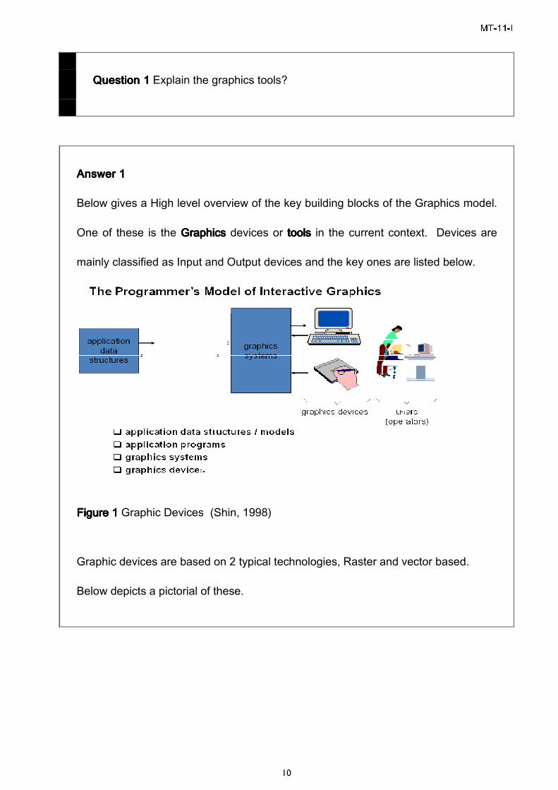
Below gives a High level overview of the key building blocks of the Graphics model.
One of these is the GraphicsGraphicsGraphicsGraphics
mainly classified as Input and Output devices and the key ones are listed below.
FigurFigurFigurFigure e e e 1111 Graphic Devices
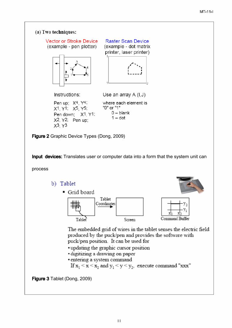
Graphic devices are based on 2 typical technologies, Raster and vector based.
Below depicts a pictorial of these.
10
Explain the graphics tools?
Below gives a High level overview of the key building blocks of the Graphics model.
GraphicsGraphicsGraphicsGraphics devices or toolstoolstoolstools in the current context. Devices are
mainly classified as Input and Output devices and the key ones are listed below.
Graphic Devices (Shin, 1998)
Graphic devices are based on 2 typical technologies, Raster and vector based.
Below depicts a pictorial of these.
MT-11-I
Below gives a High level overview of the key building blocks of the Graphics model.
in the current context. Devices are
mainly classified as Input and Output devices and the key ones are listed below.
Graphic devices are based on 2 typical technologies, Raster and vector based.
MT-11-I
11
Figure Figure Figure Figure 2222 Graphic Device Types (Dong, 2009)
Input devices:Input devices:Input devices:Input devices: Translates user or computer data into a form that the system unit can
process
Figure Figure Figure Figure 3333 Tablet (Dong, 2009)
MT-11-I
12
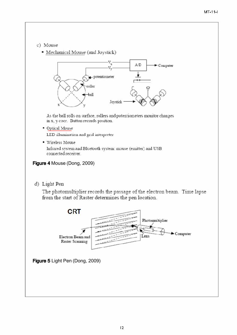
Figure Figure Figure Figure 4444 Mouse (Dong, 2009)
Figure Figure Figure Figure 5555 Light Pen (Dong, 2009)
MT-11-I
13
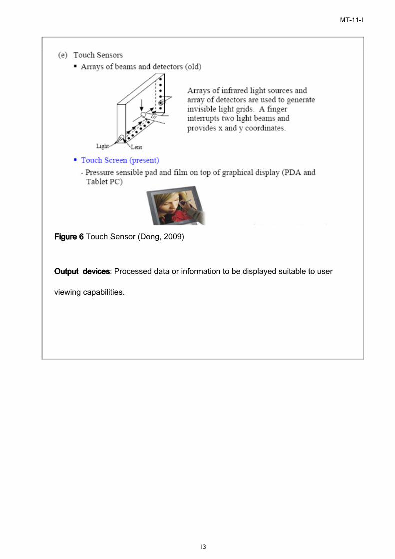
Figure Figure Figure Figure 6666 Touch Sensor (Dong, 2009)
Output devicesOutput devicesOutput devicesOutput devices: Processed data or information to be displayed suitable to user
viewing capabilities.
MT-11-I
14
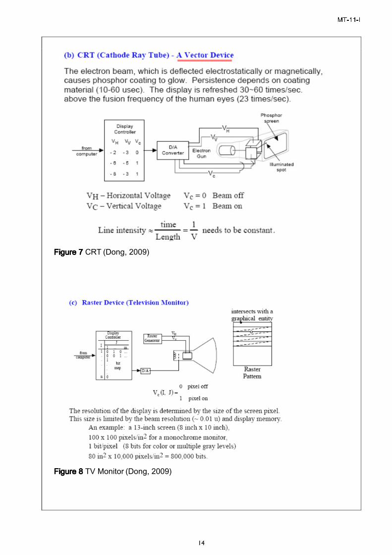
Figure Figure Figure Figure 7777 CRT (Dong, 2009)
Figure Figure Figure Figure 8888 TV Monitor (Dong, 2009)
MT-11-I
15
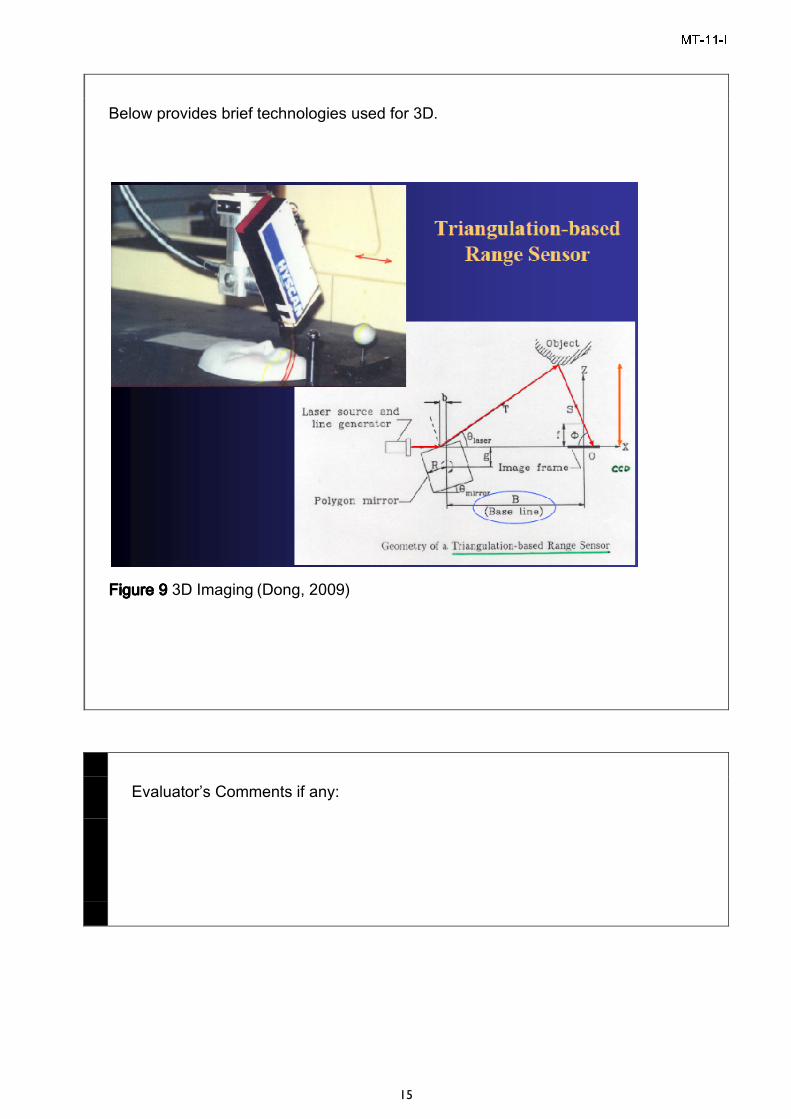
Below provides brief technologies used for 3D.
Figure Figure Figure Figure 9999 3D Imaging (Dong, 2009)
Evaluator’s Comments if any:
MT-11-I
16
Question 2Question 2Question 2Question 2 Explain Bresenham’s algorithm?
Answer 2Answer 2Answer 2Answer 2
An accurate and efficient raster line-generating algorithm, developed by
Bresenham, scan converts lines using only incrementa1 integer calculations that
can be adapted to display circles and other curves.
The Bresenham line algorithm is an algorithm which determines which points in
an n-dimensional raster should be plotted in order to form a close approximation
to a straight line between two given points. It is commonly used to draw lines on
a computer screen, as it uses only integer addition, subtraction and bit shifting,
all of which are very cheap operations in standard computer architectures. It is
one of the earliest algorithms developed in the field of computer graphics. A
minor extension to the original algorithm also deals with drawing circles.
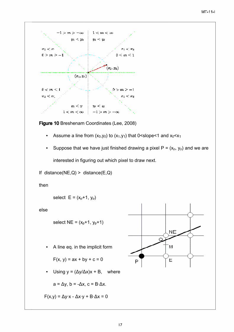
Figure Figure Figure Figure 10101010 Breshenam Coordinates
• Assume a line from (x
• Suppose that we have just finished drawing a pixel P = (x
interested in figuring out which pixel to draw next.
If distance(NE,Q) > distance(E,Q)
then
select E = (xp+1, y
else
select NE = (xp+1, y
• A line eq. in the implicit form
F(x, y) = ax + by + c = 0
• Using y = (Δy/Δx)x + B, where
a = Δy, b = -Δx, c =
F(x,y) = Δy·x - Δx·y + B·Δx = 0
17
Breshenam Coordinates (Lee, 2008)
Assume a line from (x0,y0) to (x1,y1) that 0<slope<1 and x
Suppose that we have just finished drawing a pixel P = (x
figuring out which pixel to draw next.
If distance(NE,Q) > distance(E,Q)
+1, yp) +1, yp+1)
A line eq. in the implicit form
F(x, y) = ax + by + c = 0
Using y = (Δy/Δx)x + B, where
Δx, c = B·Δx.
Δx·y + B·Δx = 0
MT-11-I
) that 0<slope<1 and x0<x1 Suppose that we have just finished drawing a pixel P = (xp, yp) and we are
MT-11-I
18
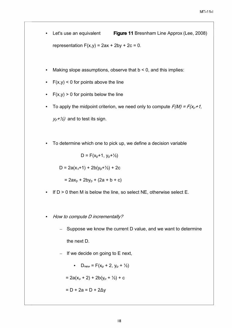
• Let's use an equivalent
representation F(x,y) = 2ax + 2by + 2c = 0.
• Making slope assumptions, observe that b < 0, and this implies:
• F(x,y) < 0 for points above the line
• F(x,y) > 0 for points below the line
• To apply the midpoint criterion, we need only to compute F(M) = F(xp+1,
yp+½) and to test its sign.
• To determine which one to pick up, we define a decision variable
D = F(xp+1, yp+½)
D = 2a(xp+1) + 2b(yp+½) + 2c
= 2axp + 2byp + (2a + b + c)
• If D > 0 then M is below the line, so select NE, otherwise select E.
• How to compute D incrementally?
– Suppose we know the current D value, and we want to determine
the next D.
– If we decide on going to E next,
• Dnew = F(xp + 2, yp + ½)
= 2a(xp + 2) + 2b(yp + ½) + c
= D + 2a = D + 2Δy
Figure Figure Figure Figure 11111111 Bresnham Line Approx (Lee, 2008)
MT-11-I
19
– If we decide on going to NE next,
• Dnew = F(xp + 2, yp + 1 + ½)
= 2a(xp + 2) + 2b(yp + 1 + ½) + c
= D + 2(a + b) = D + 2(Δy - Δx).
• Since we start at (x0,y0), the initial value of D can be calculated by
Dinit = F(x0 + 1, y0 + ½)
= (2ax0 + 2by0 + c) + (2a + b)
= 0 + 2a + b
= 2Δy - Δx
• Advantages
– need to add integers and multiply by 2
(which can be done by shift operations)
– incremental algorithm
Example:
Line end points:
MT-11-I
20
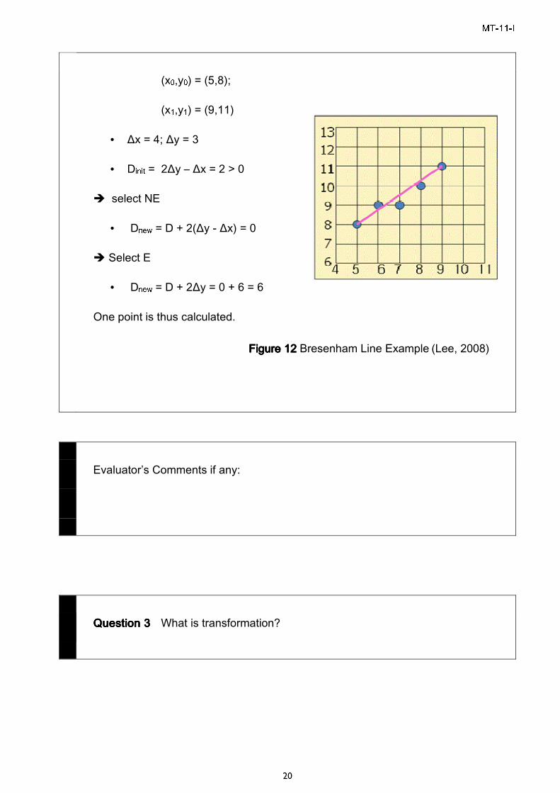
(x0,y0) = (5,8);
(x1,y1) = (9,11)
• Δx = 4; Δy = 3
• Dinit = 2Δy – Δx = 2 > 0
� select NE
• Dnew = D + 2(Δy - Δx) = 0
� Select E
• Dnew = D + 2Δy = 0 + 6 = 6
One point is thus calculated.
Evaluator’s Comments if any:
Question 3Question 3Question 3Question 3 What is transformation?
Figure Figure Figure Figure 12121212 Bresenham Line Example (Lee, 2008)
MT-11-I
21
Answer 3Answer 3Answer 3Answer 3
With the procedures for displaying output primitives and their attributes, we can
create variety of pictures and graphs. In many applications, there is also a need for
altering or manipulating displays. Design applications and facility layouts are created
by arranging the orientations and sizes of the component parts of the scene. And
animations are produced by moving the "camera" or the objects in a scene along
animation paths. Changes in orientation, size, and shape are accomplished with
geometric transformations that alter the coordinate descriptions of objects. The
basic geometric transformations are translation, rotation, and scaling. Other
transformations that are often applied to objects include reflection and shear.
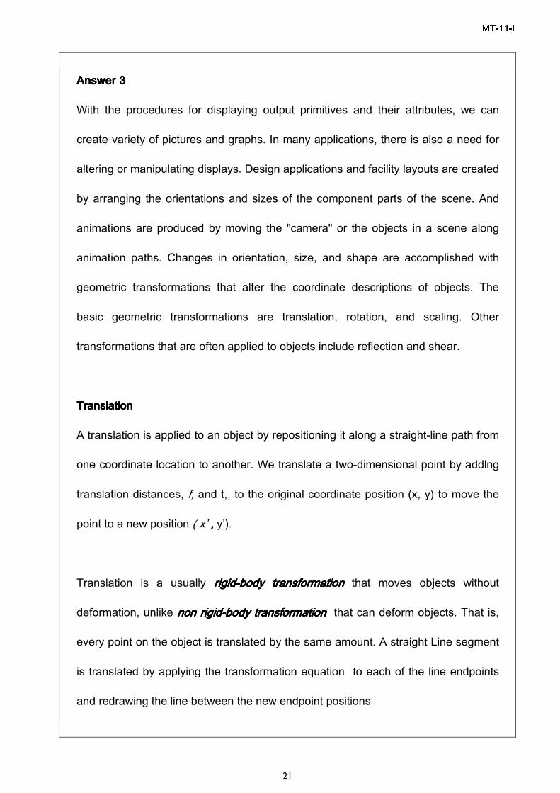
TranslationTranslationTranslationTranslation
A translation is applied to an object by repositioning it along a straight-line path from
one coordinate location to another. We translate a two-dimensional point by addlng
translation distances, f, and t,, to the original coordinate position (x, y) to move the
point to a new position ( x’ , , , , y’).
Translation is a usually rigidrigidrigidrigid----body transformbody transformbody transformbody transformaaaation tion tion tion that moves objects without
deformation, unlike non rigidnon rigidnon rigidnon rigid----body transformationbody transformationbody transformationbody transformation that can deform objects. That is,
every point on the object is translated by the same amount. A straight Line segment
is translated by applying the transformation equation to each of the line endpoints
and redrawing the line between the new endpoint positions
MT-11-I
22
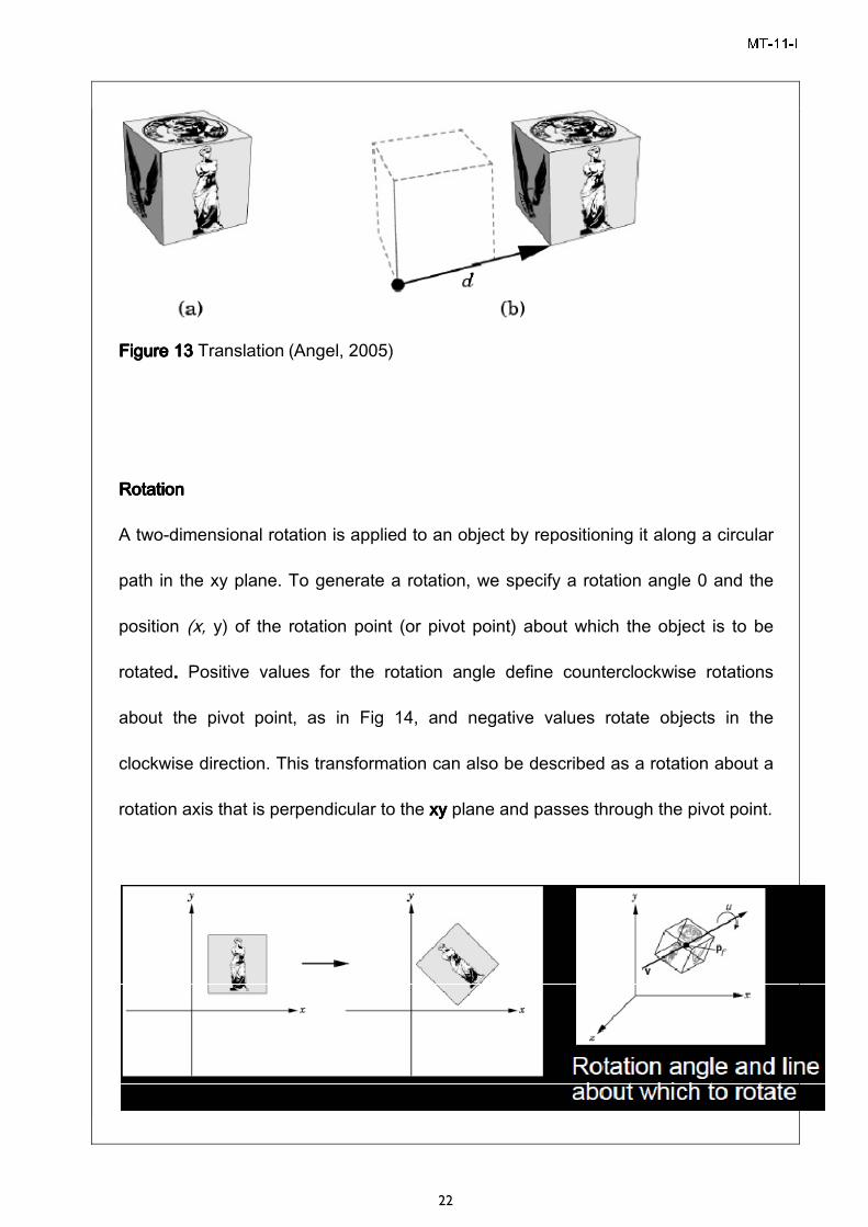
RotationRotationRotationRotation
A two-dimensional rotation is applied to an object by repositioning it along a circular
path in the xy plane. To generate a rotation, we specify a rotation angle 0 and the
position (x, y) of the rotation point (or pivot point) about which the object is to be
rotated.... Positive values for the rotation angle define counterclockwise rotations
about the pivot point, as in Fig 14, and negative values rotate objects in the
clockwise direction. This transformation can also be described as a rotation about a
rotation axis that is perpendicular to the xy xy xy xy plane and passes through the pivot point.
Figure Figure Figure Figure 13131313 Translation (Angel, 2005)
MT-11-I
23
Figure Figure Figure Figure 14141414 Rotation (Angel, 2005)
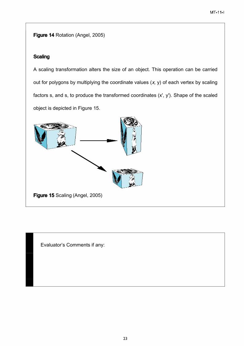
ScalingScalingScalingScaling
A scaling transformation alters the size of an object. This operation can be carried
out for polygons by multiplying the coordinate values (x, y) of each vertex by scaling
factors s, and s, to produce the transformed coordinates (x', y'). Shape of the scaled
object is depicted in Figure 15.
Figure Figure Figure Figure 15151515 Scaling (Angel, 2005)
Evaluator’s Comments if any:
MT-11-I
24
Question 4Question 4Question 4Question 4 Explain need for clipping and windowing?
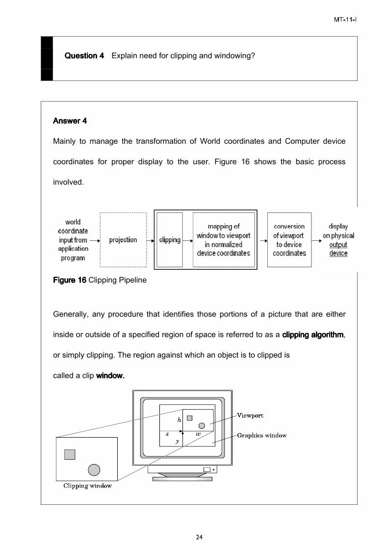
Answer 4Answer 4Answer 4Answer 4
Mainly to manage the transformation of World coordinates and Computer device
coordinates for proper display to the user. Figure 16 shows the basic process
involved.
Figure Figure Figure Figure 16161616 Clipping Pipeline
Generally, any procedure that identifies those portions of a picture that are either
inside or outside of a specified region of space is referred to as a clipping clipping clipping clipping algoalgoalgoalgorithmrithmrithmrithm,
or simply clipping. The region against which an object is to clipped is
called a clip window.window.window.window.
MT-11-I
25
Figure Figure Figure Figure 17171717 Clipping
Applications of clipping include extracting part of a detained scene for viewing;
identifying visible surfaces in three-dimensional views; antialiasing line segments or
object boundaries; creating objects using solid-modeling procedures;
displaying a multiwindow environment; and drawing and painting operations that
allow parts of a picture to be selected for copying, moving, erasing, or duplicating.
Depending on the application, the clip window can be a general polygon or it can
even have curved boundaries.
Evaluator’s Comments if any:
Question 5Question 5Question 5Question 5 What is Sutherland - Hodgeman algorithm?
Answer 5Answer 5Answer 5Answer 5
Similarly to lines, areas must be clipped to a window boundary.
Consideration must be taken as to which portions of the area must be clipped.
MT-11-I
26
A technique for clipping areas developed by Sutherland & Hodgman. Put simply
the polygon is clipped by comparing it against each boundary in turn.
We can correctly clip a polygon by processing the polygon boundary as a whole
against each window edge. This could be accomplished by processing all polygon
vertices against each clip rectangle boundary in turn. Beginning with the initial set
of polygon vertices, we could first clip the polygon against the left rectangle
boundary to produce a new sequence of vertices. The new set of vertices could
then k successively passed to a right boundary clipper, a bottom boundary clipper,
and a top boundary clipper, as in Fig. 18. At each step, a new sequence of output
vertices is generated and passed to the next window boundary clipper.
There are four possible cases when processing vertices in sequence around the
perimeter of a polygon. As each pair of adjacent polygon vertices is passed to a
window boundary clipper, we make the following tests:
(1) If the first vertex is outside the window boundary and the second vertex is
inside, both the intersection point of the polygon edge with the window boundary
and the second vertex are added to the output vertex list.
(2) If both input vertices are inside the window boundary, only the second vertex is
added to the output vertex list.
(3) li the first vertex is inside the window boundary and the second vertex is
outside, only the edge intersection with the window boundary is added to the
output vertex list.

MT-11-I
27
(4) If both input vertices are outside the window boundary, nothing is added to the
output list. These four cases are illustrated in Fig. 18 for successive pairs of
polygon vertices. Once all vertices have been processed for one clip window
boundary, the output list of vertices is clipped against the next window boundary.
Figure Figure Figure Figure 18181818 Sutherland-Hodgman Area Clipping
Evaluator’s Comments if any:
Question 6Question 6Question 6Question 6 Describe rubber band techniques?
Answer 6Answer 6Answer 6Answer 6
Straight lines can be constructed and positioned using rrrrubberubberubberubber----band band band band methods,
which stretch out a line from a starting position as the screen cursor is moved.
Figure 19 demonstrates the rubber-band method. We first select a screen
MT-11-I
28
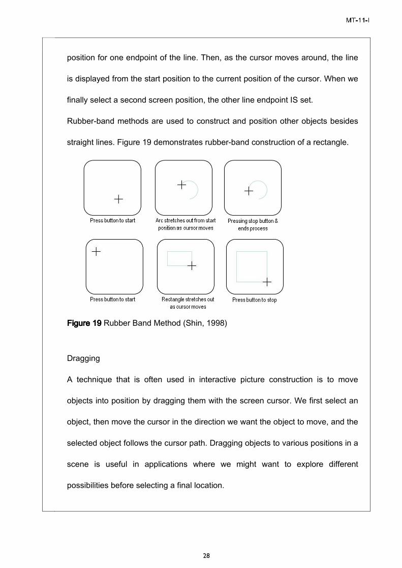
position for one endpoint of the line. Then, as the cursor moves around, the line
is displayed from the start position to the current position of the cursor. When we
finally select a second screen position, the other line endpoint IS set.
Rubber-band methods are used to construct and position other objects besides
straight lines. Figure 19 demonstrates rubber-band construction of a rectangle.
Figure Figure Figure Figure 19191919 Rubber Band Method (Shin, 1998)
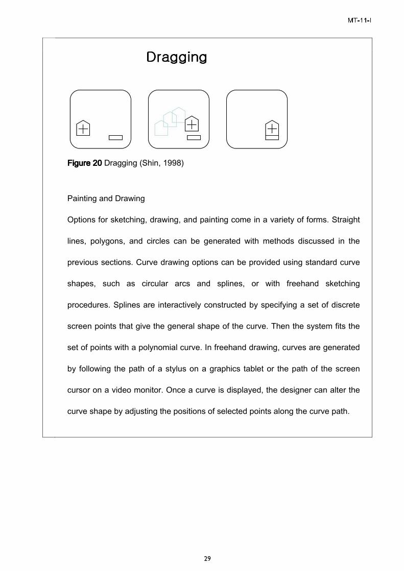
Dragging
A technique that is often used in interactive picture construction is to move
objects into position by dragging them with the screen cursor. We first select an
object, then move the cursor in the direction we want the object to move, and the
selected object follows the cursor path. Dragging objects to various positions in a
scene is useful in applications where we might want to explore different
possibilities before selecting a final location.
MT-11-I
29
Figure Figure Figure Figure 20202020 Dragging (Shin, 1998)
Painting and Drawing
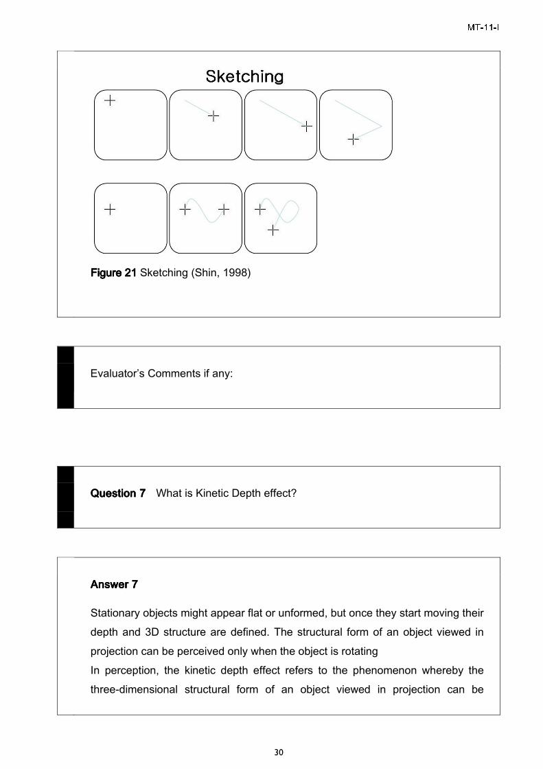
Options for sketching, drawing, and painting come in a variety of forms. Straight
lines, polygons, and circles can be generated with methods discussed in the
previous sections. Curve drawing options can be provided using standard curve
shapes, such as circular arcs and splines, or with freehand sketching
procedures. Splines are interactively constructed by specifying a set of discrete
screen points that give the general shape of the curve. Then the system fits the
set of points with a polynomial curve. In freehand drawing, curves are generated
by following the path of a stylus on a graphics tablet or the path of the screen
cursor on a video monitor. Once a curve is displayed, the designer can alter the
curve shape by adjusting the positions of selected points along the curve path.
MT-11-I
30
Figure Figure Figure Figure 21212121 Sketching (Shin, 1998)
Evaluator’s Comments if any:
Question 7Question 7Question 7Question 7 What is Kinetic Depth effect?
Answer 7Answer 7Answer 7Answer 7
Stationary objects might appear flat or unformed, but once they start moving their depth and 3D structure are defined. The structural form of an object viewed in projection can be perceived only when the object is rotating In perception, the kinetic depth effect refers to the phenomenon whereby the three-dimensional structural form of an object viewed in projection can be
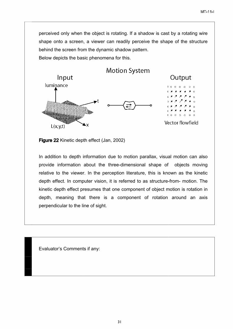
perceived only when the object is rotating. If a shadow is cast by a rotating wire shape onto a screen, a vbehind the screen from the dynamic shadow pattern.Below depicts the basic phenomena for this.
Figure Figure Figure Figure 22222222 Kinetic depth In addition to depth information due to motion parallax, visual motion can also provide information about the threerelative to the viewer. In the perception literature, this is known asdepth effect. In computkinetic depth effect presumes that one component of object motion is rotation in depth, meaning that there is a component of rotation around an axisperpendicular to the line of sight.
Evaluator’s Comments if any:
31
perceived only when the object is rotating. If a shadow is cast by a rotating wire shape onto a screen, a viewer can readily perceive the shape of the structure behind the screen from the dynamic shadow pattern. Below depicts the basic phenomena for this.
Kinetic depth effect (Jan, 2002)
addition to depth information due to motion parallax, visual motion can also provide information about the three-dimensional shape of objects moving relative to the viewer. In the perception literature, this is known asdepth effect. In computer vision, it is referred to as structure-kinetic depth effect presumes that one component of object motion is rotation in depth, meaning that there is a component of rotation around an axisperpendicular to the line of sight.
Evaluator’s Comments if any:
MT-11-I perceived only when the object is rotating. If a shadow is cast by a rotating wire
iewer can readily perceive the shape of the structure
addition to depth information due to motion parallax, visual motion can also dimensional shape of objects moving
relative to the viewer. In the perception literature, this is known as the kinetic -from- motion. The
kinetic depth effect presumes that one component of object motion is rotation in depth, meaning that there is a component of rotation around an axis
MT-11-I
32
Question 8Question 8Question 8Question 8 What are Singularities? Describe algorithm Singularity
Answer 8Answer 8Answer 8Answer 8
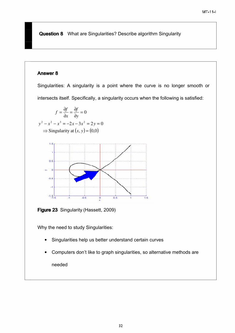
Singularities: A singularity is a point where the curve is no longer smooth or
intersects itself. Specifically, a singularity occurs when the following is satisfied:
( ) ( )0,0,at y Singularit
0232
0
2322
=⇒
==−−=−−
=∂
∂=
∂
∂=
yx
yxxxxy
y
f
x
ff
Figure Figure Figure Figure 23232323 Singularity (Hassett, 2009)
Why the need to study Singularities:
• Singularities help us better understand certain curves
• Computers don’t like to graph singularities, so alternative methods are
needed
MT-11-I
33
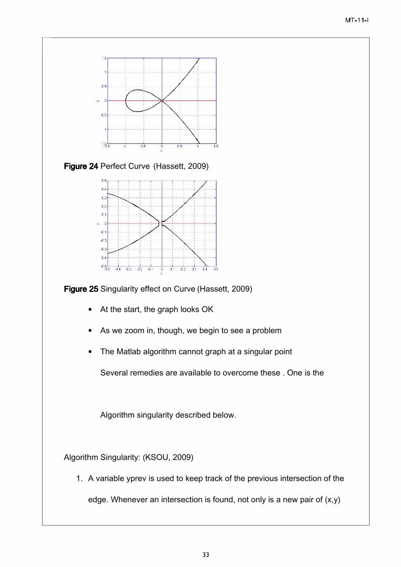
Figure Figure Figure Figure 24242424 Perfect Curve (Hassett, 2009)
Figure Figure Figure Figure 25252525 Singularity effect on Curve (Hassett, 2009)
• At the start, the graph looks OK
• As we zoom in, though, we begin to see a problem
• The Matlab algorithm cannot graph at a singular point
Several remedies are available to overcome these . One is the
Algorithm singularity described below.
Algorithm Singularity: (KSOU, 2009)
1. A variable yprev is used to keep track of the previous intersection of the
edge. Whenever an intersection is found, not only is a new pair of (x,y)
MT-11-I
34
stored as in the yx algorithm, but the y coordinate is stored to indicate the
previous intersection by storing it in yprev. Initially its value is set to 0.
2. Go to the next edge of the polygon. If these are no more edges to be
processed, exit.
3. Compute its intersection with the scan lines. If it has no intersections at all
it can be considered horizontal. Go to step 2.
4. Compute the difference dy=y2-y1, where y2 is the y coordinate of the
beginning vertex of the edge and y1 the y coordinate of the ending vertex.
If dy >0 go to step 5, else go to step 6.
5. If dy>0 the first intersection generated must have y=yprev+1, compute all
other intersections of the edge. The y coordinate of the last intersection is
stored in yprev. Go to step 2 to findout whether any edges are still there.
6. F dy<0 the first intersection generated will have y= yprev itself generate all
intersections for the edge. The y coordinate of the last intersection is
preserved in the yprev=ylast-1. Go to step 2.
Note that this algorithm does not generate intersection nor does it produce the
scan conversion. The scan conversion algorithm, which does the conversion, will
only pass its intersection values to the singularity algorithm to check for the
specific cases.
MT-11-I
35
Evaluator’s Comments if any:
Question 9Question 9Question 9Question 9 Explain the 3-d transformation
Answer 9Answer 9Answer 9Answer 9
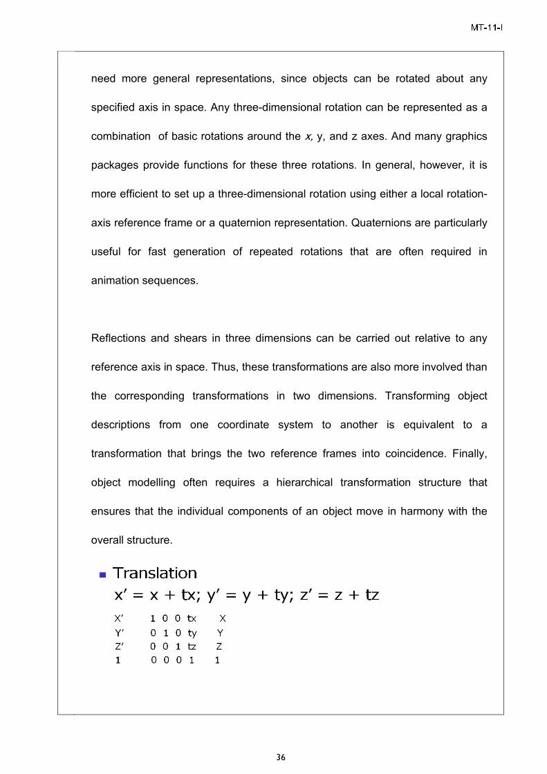
Three-dimensional transformations useful in computer graphics applications
include geometric transformations within a single coordinate system and
transformations between different coordinate systems. The basic geometric
transformations are translation, rotation, and scaling. Two additional object
transformations are reflections and shears. Transformations between different
coordinate systems are common elements of modeling and viewing routines. In
three dimensions, transformation operations are represented with 4 by 4
matrices. As in two-dimensional graphics methods, a composite transformation
in three-dimensions is obtained by concatenating the matrix representations for
the individual components of the overall transformation.
Representations for translation and scaling are straightforward extensions of
two-dimensional transformation representations. For rotations, however, we
MT-11-I
36
need more general representations, since objects can be rotated about any
specified axis in space. Any three-dimensional rotation can be represented as a
combination of basic rotations around the x, y, and z axes. And many graphics
packages provide functions for these three rotations. In general, however, it is
more efficient to set up a three-dimensional rotation using either a local rotation-
axis reference frame or a quaternion representation. Quaternions are particularly
useful for fast generation of repeated rotations that are often required in
animation sequences.
Reflections and shears in three dimensions can be carried out relative to any
reference axis in space. Thus, these transformations are also more involved than
the corresponding transformations in two dimensions. Transforming object
descriptions from one coordinate system to another is equivalent to a
transformation that brings the two reference frames into coincidence. Finally,
object modelling often requires a hierarchical transformation structure that
ensures that the individual components of an object move in harmony with the
overall structure.
MT-11-I
37
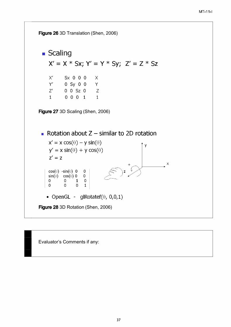
Figure Figure Figure Figure 26262626 3D Translation (Shen, 2006)
Figure Figure Figure Figure 27272727 3D Scaling (Shen, 2006)
Figure Figure Figure Figure 28282828 3D Rotation (Shen, 2006)
Evaluator’s Comments if any:
MT-11-I
38
Question 10Question 10Question 10Question 10 Explain Warnock’s algorithm
Answer 10Answer 10Answer 10Answer 10
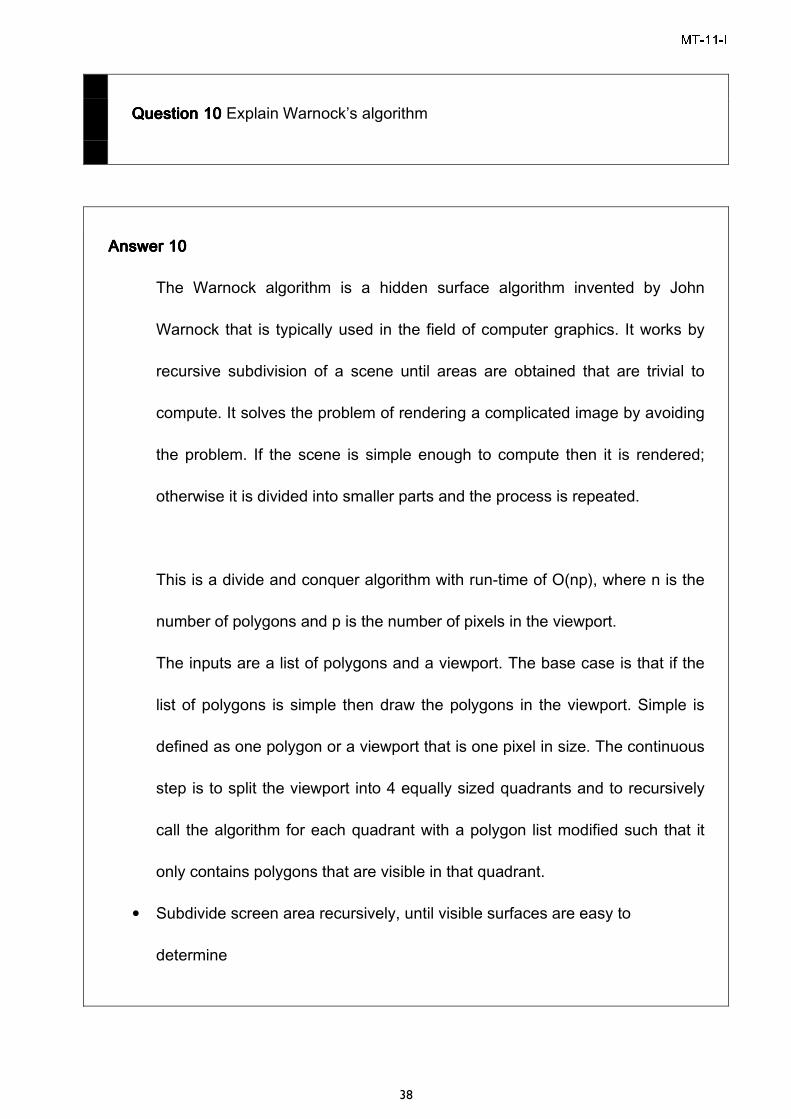
The Warnock algorithm is a hidden surface algorithm invented by John
Warnock that is typically used in the field of computer graphics. It works by
recursive subdivision of a scene until areas are obtained that are trivial to
compute. It solves the problem of rendering a complicated image by avoiding
the problem. If the scene is simple enough to compute then it is rendered;
otherwise it is divided into smaller parts and the process is repeated.
This is a divide and conquer algorithm with run-time of O(np), where n is the
number of polygons and p is the number of pixels in the viewport.
The inputs are a list of polygons and a viewport. The base case is that if the
list of polygons is simple then draw the polygons in the viewport. Simple is
defined as one polygon or a viewport that is one pixel in size. The continuous
step is to split the viewport into 4 equally sized quadrants and to recursively
call the algorithm for each quadrant with a polygon list modified such that it
only contains polygons that are visible in that quadrant.
• Subdivide screen area recursively, until visible surfaces are easy to
determine
MT-11-I
39
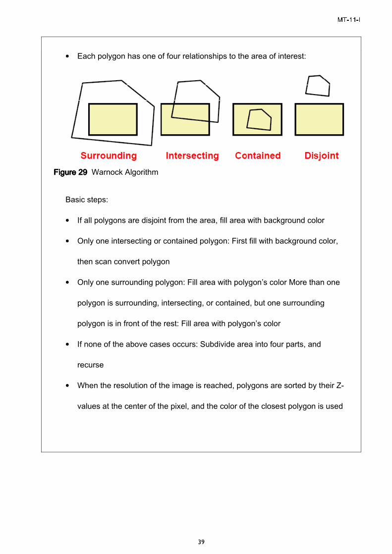
• Each polygon has one of four relationships to the area of interest:
Figure Figure Figure Figure 29292929 Warnock Algorithm
Basic steps:
• If all polygons are disjoint from the area, fill area with background color
• Only one intersecting or contained polygon: First fill with background color,
then scan convert polygon
• Only one surrounding polygon: Fill area with polygon’s color More than one
polygon is surrounding, intersecting, or contained, but one surrounding
polygon is in front of the rest: Fill area with polygon’s color
• If none of the above cases occurs: Subdivide area into four parts, and
recurse
• When the resolution of the image is reached, polygons are sorted by their Z-
values at the center of the pixel, and the color of the closest polygon is used
MT-11-I
40
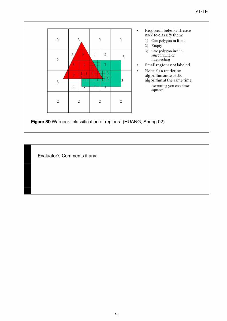
Figure Figure Figure Figure 30303030 Warnock- classification of regions (HUANG, Spring 02)
Evaluator’s Comments if any:

MT-11-I
41
BibliographyBibliographyBibliographyBibliography Angel, E. (2005). Transformations. Mexico: Electrical and Computer Engineering, University of Mexico.
Dong, Z. (2009). Hardware of a CAD System. British Colombia,Canada: University of Victory, Mechnical Engineering.
Hassett, D. B. (2009). Resolving Singularities. USA: Rice University.
HUANG, J. (Spring 02). CS594 Visualization & Adv. Computer Graphics. Wisconsin: University of Wisconsin.
Jan, C. (2002). Mechanisms of Motion Perception . Irvine: University of California.
KSOU. (2009). Interactive computer graphics. Delhi: Virtual Education trust.
Lee, J. (2008). Output Primitives. Seoul, South Korea: Seoul National University.
Shen, H.-W. (2006). CSE581: Interactive Computer Graphics . Ohio: The Ohio State University .
Shin, S. Y. (1998). CS580 Computer Graphics. South Korea: Korea Advanced Institute of Science and Technology.