Embed Size (px)
Citation preview
Graphics Lecture 4: Slide 1
Interactive Computer Graphics
Lecture 4: Colour

Graphics Lecture 4: Slide 2
Ways of looking at colour
1. Physics
2. Human visual receptors
3. Subjective assessment

Graphics Lecture 4: Slide 3
The physics of colour
A pure colour is a wave with:
Wavelength ()
Amplitude (intensity or energy) (I)

Graphics Lecture 8: Slide 4

Graphics Lecture 4: Slide 5
Colours are energy distributions
Lasers are light sources that contain a single wavelength (or a very narrow band of wavelengths)
In practice light is made up of a mixture of many wavelengths with an energy distribution.

Graphics Lecture 4: Slide 6
Light distribution for red
Energy
300 nm (violet)
Wavelength
Light distribution perceived as red
700 nm (red)

Graphics Lecture 4: Slide 7
Sunlight
Energy
300 nm(violet)
500 nm(green)
700 nm(red)
Wavelength
Light energy distribution in sunlight

Graphics Lecture 4: Slide 8
Human Colour Vision
Human colour vision is based on three ‘cone’ cell types which respond to light energy in different bands of wavelength.
The bands overlap in a curious manner.
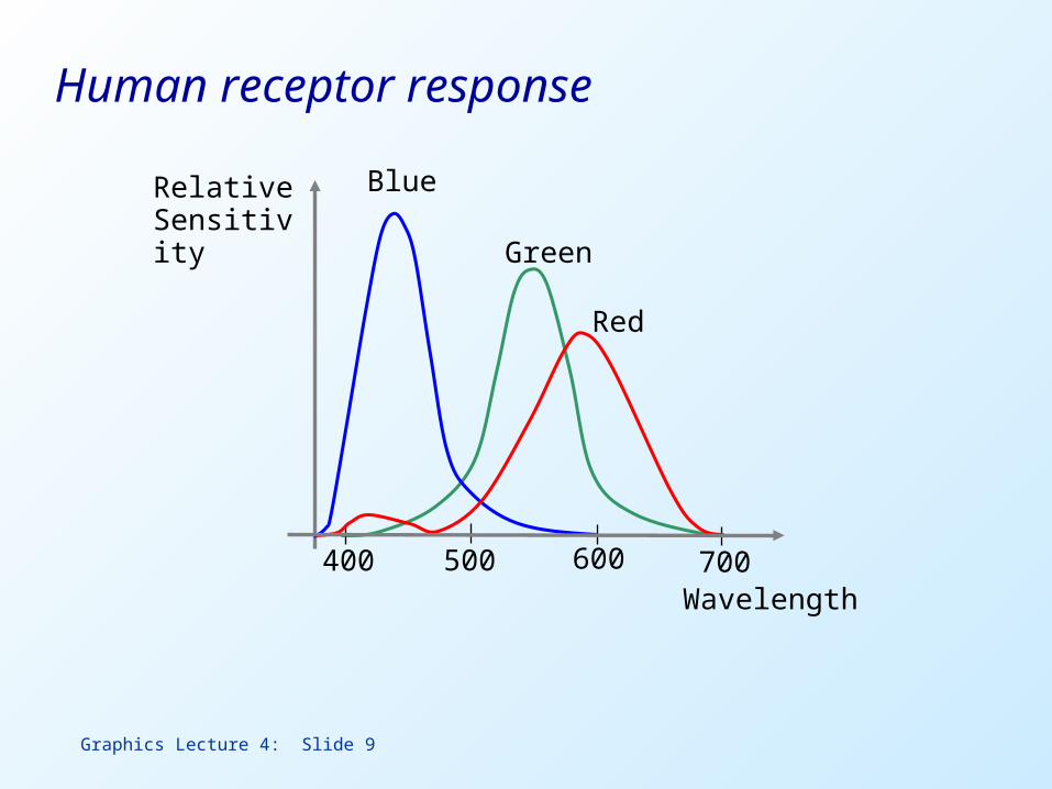
Graphics Lecture 4: Slide 9
Human receptor response
400 500 600 700
Blue
Green
Red
Wavelength
RelativeSensitivity
Graphics Lecture 4: Slide 10
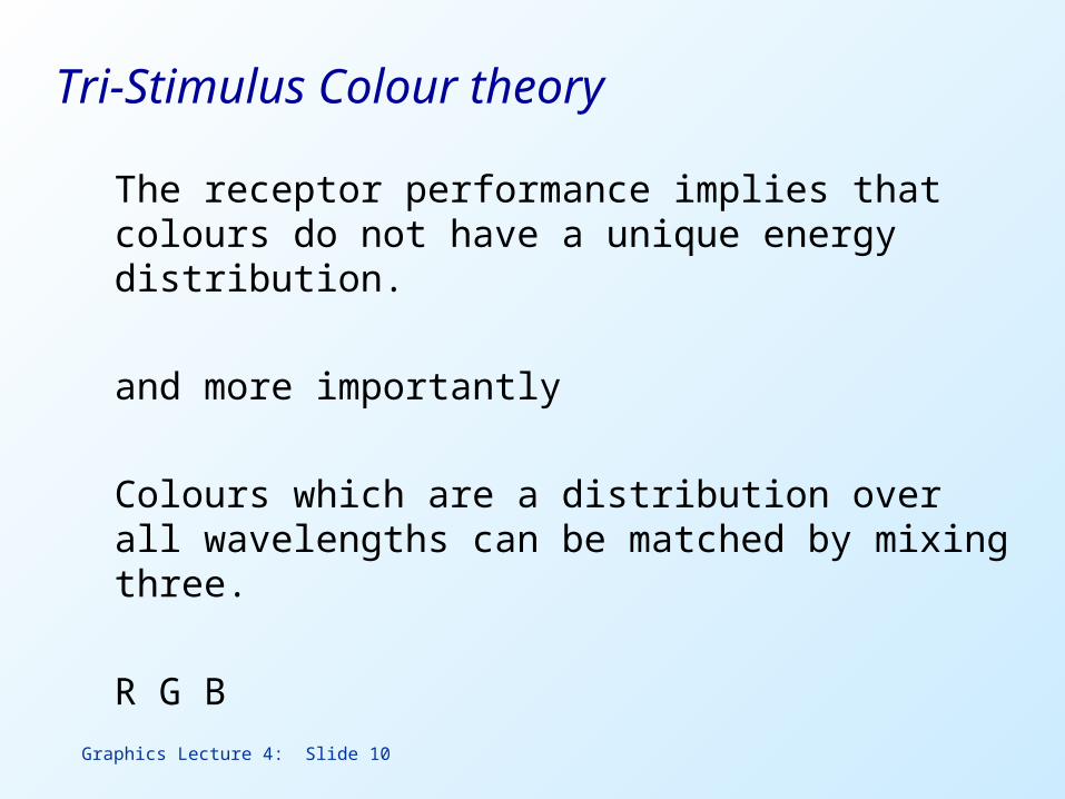
Tri-Stimulus Colour theory
The receptor performance implies that colours do not have a unique energy distribution.
and more importantly
Colours which are a distribution over all wavelengths can be matched by mixing three.
R G B

Graphics Lecture 4: Slide 11
Colour Matching
Given any colour light source, regardless of the distribution of wavelengths that it contains, we can try to match it with a mixture of three light sources
X = r R + g G + b B
where R, G and B are pure light sources and r, g and b their intensities
For simplicity we can drop the R G B.
Graphics Lecture 4: Slide 12
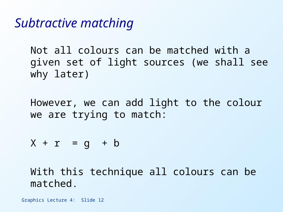
Subtractive matching
Not all colours can be matched with a given set of light sources (we shall see why later)
However, we can add light to the colour we are trying to match:
X + r = g + b
With this technique all colours can be matched.
Graphics Lecture 4: Slide 13
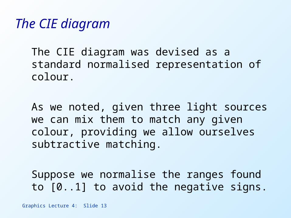
The CIE diagram
The CIE diagram was devised as a standard normalised representation of colour.
As we noted, given three light sources we can mix them to match any given colour, providing we allow ourselves subtractive matching.
Suppose we normalise the ranges found to [0..1] to avoid the negative signs.

Graphics Lecture 4: Slide 14
Normalised colours
Having normalised the range over which the matching is done we can now normalise the colours such that the three components sum to 1.
thus x = r/(r+g+b)
y = g/(r+g+b)
z = b/(r+g+b) = 1 - x - y
We can now represent all our colours in a 2D space.

Graphics Lecture 4: Slide 15
Defining the normalised CIE diagram
0.0
1.0
1.0
Y
X
Hypothetical Green Source
Hypothetical Red Source
Hypothetical Blue Source
Standard observer response accounting for the cone cell densities in a solid angle
400 700600500
0.5
2.0
1.5
1.0
(nm)
Z (blue)
Y (green)
X (red)

Graphics Lecture 4: Slide 16
Actual Visible Colours
0.8
0.6
0.4
0.2
0 0.2 0.4x
y
0.6 0.8
520530
510
500
490
480
380
550
570
590
620
780
400 700600500
0.5
2.0
1.5
1.0
(nm)
Z (blue)
Y (green)X
(red)
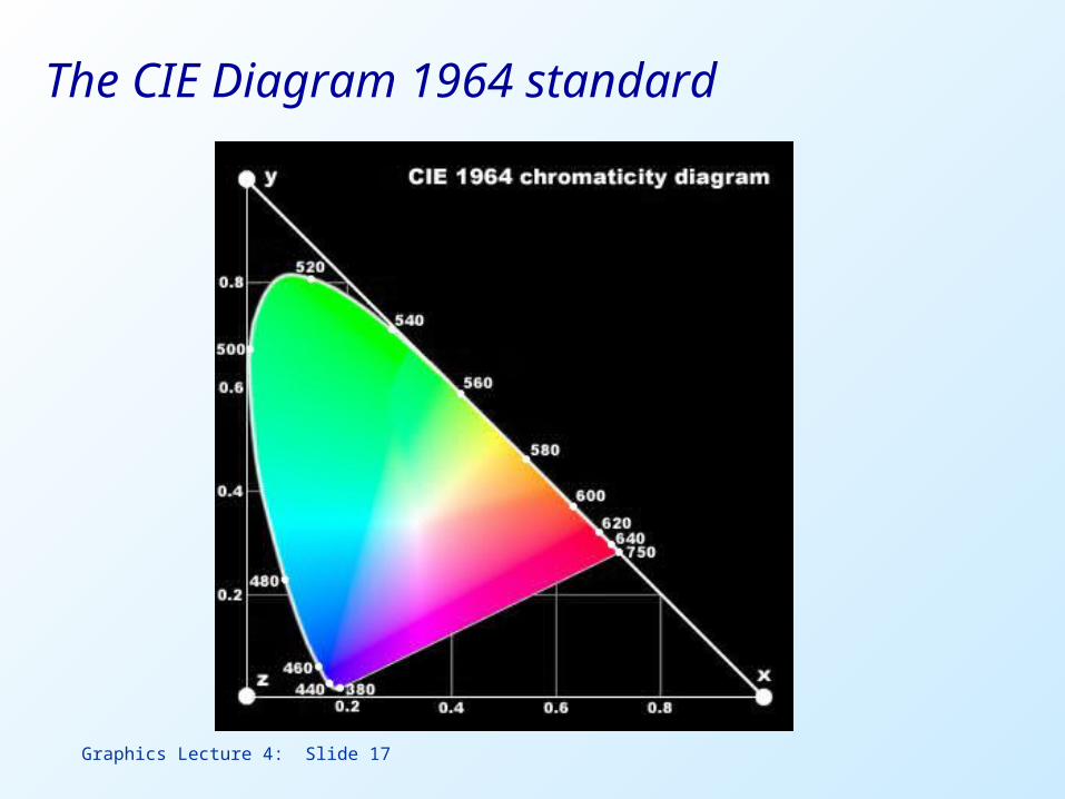
Graphics Lecture 4: Slide 17
The CIE Diagram 1964 standard

Graphics Lecture 4: Slide 18
Convex Shape
Notice that the pure colours (coherent ) are round the edge of the CIE diagram.
The shape must be convex, since any blend (interpolation) of pure colours should create a colour in the visible region.
The line joining purple and red has no pure equivalent. The colours can only be created by blending.
Graphics Lecture 4: Slide 19
Intensities
Since the colours are all normalised there is no representation of intensity.
By changing the intensity perceptually different colours can be seen.
Graphics Lecture 4: Slide 20
White Point
When the three colour components are equal, the colour is white:
x = 0.33
y = 0.33
This point is clearly visible on the CIE diagram
Graphics Lecture 4: Slide 21
Saturation
Pure colours are called fully saturated.
These correspond to the colours around the edge of the horseshoe.
Saturation of a arbitrary point is the ratio of its distance to the white point over the distance of the white point to the edge.

Graphics Lecture 4: Slide 22
Complement Colour
The complement of a fully saturated colour is the point diametrically opposite through the white point.
A colour added to its complement gives us white.

Graphics Lecture 4: Slide 23
Actual Visible Colours
0.8
0.6
0.4
0.2
0 0.2 0.4x
y
0.6 0.8
520
530
510
500
490
480
380
550
570
590
620
780
Complement Colour (C)
White Point (W)
Pure Colour (P)
Unsaturated Colour (U)

Graphics Lecture 4: Slide 24
Subtractive Primaries
When printing colour we use a subtractive representation.
Inks absorb wavelengths from the incident light, hence they subtract components to create the colour.
The subtractive primaries are Magenta (purple) Cyan (light Blue) Yellow
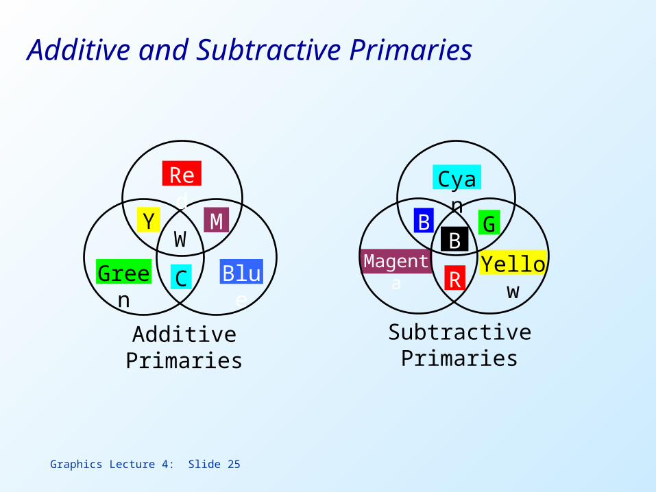
Graphics Lecture 4: Slide 25
Red
Green BlueC
Y MW
Additive Primaries
YellowMagenta
Cyan
R
B GB
Subtractive Primaries
Additive and Subtractive Primaries

Graphics Lecture 4: Slide 26
Additive vs Subtractive Colour representation
Surprisingly, the subtractive representation is capable of representing far more of the colour space than the additive.
We will see why this is so shortly.
Graphics Lecture 4: Slide 27
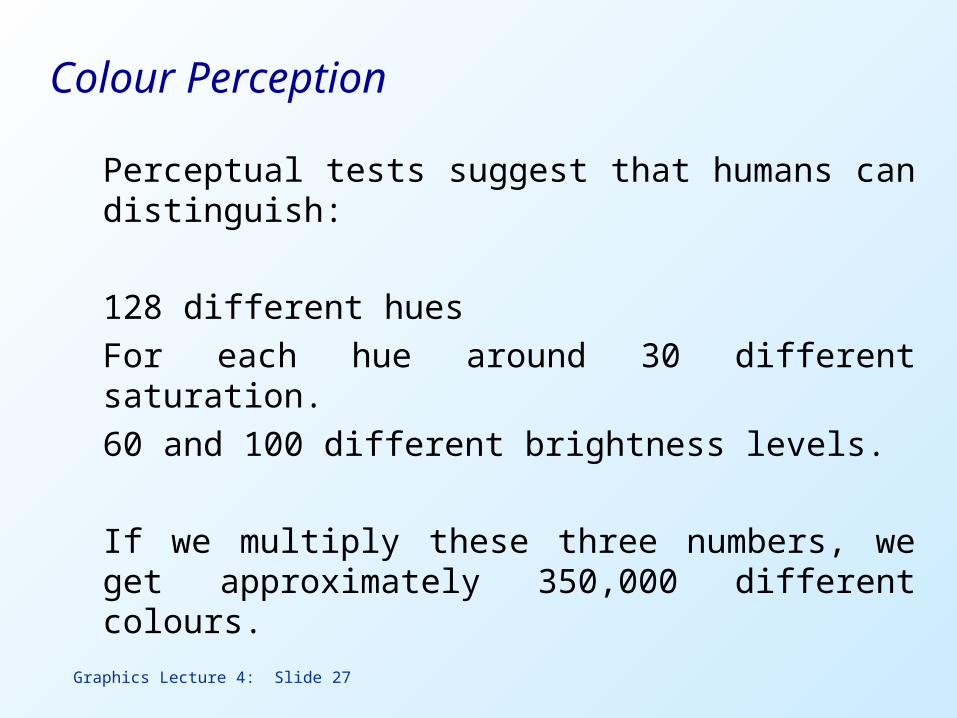
Colour Perception
Perceptual tests suggest that humans can distinguish:
128 different hues For each hue around 30 different saturation. 60 and 100 different brightness levels.
If we multiply these three numbers, we get approximately 350,000 different colours.

Graphics Lecture 4: Slide 28
Colour Perception
These figures must be treated with caution since there seems to be a much greater sensitivity to differentials in colour.
Never the less, a representation with 24 bits (8 bits for red, 8 bits for green and 8 bits for blue does provide satisfactory results.

Graphics Lecture 4: Slide 29
Reproducible colours
Colour monitors are based on adding three the output of three different light emitting phosphors or diodes.
The nominal position of these on the CIE diagram is given by:
x y z Red 0.628 0.346 0.026 Green0.268 0.588 0.144 Blue 0.150 0.07 0.780

Graphics Lecture 4: Slide 30
Actual Visible Colours
0.8
0.6
0.4
0.2
0 0.2 0.4x
y
0.6 0.8
520
530
510
500
490
480
380
550
570
590
620
700
[0.27, 0.59]
[0.63, 0.35]
[0.15, 0.07]
Display Colours

Graphics Lecture 4: Slide 31
RGB to CIE
The monitor RGB representation is related to the CIE colours by the equation:
(x, y, z) = 0.628 0.268 0.15 R 0.346 0.588 0.07 G 0.026 0.144 0.78 B
Graphics Lecture 4: Slide 32
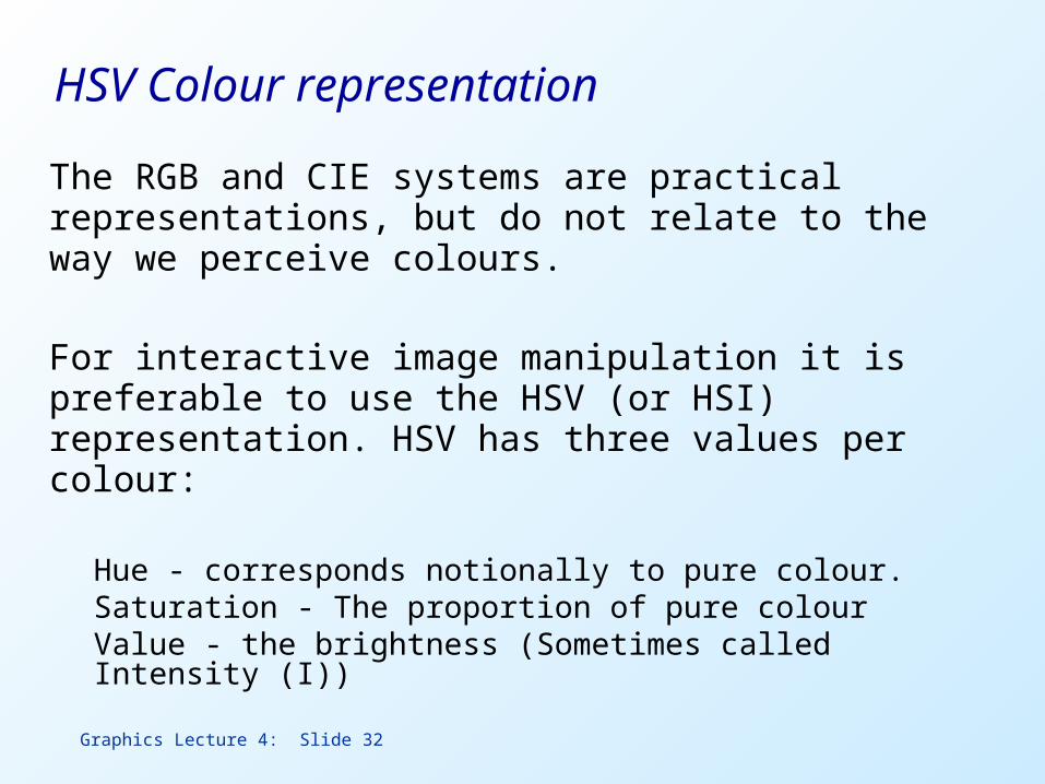
HSV Colour representation
The RGB and CIE systems are practical representations, but do not relate to the way we perceive colours.
For interactive image manipulation it is preferable to use the HSV (or HSI) representation. HSV has three values per colour:
Hue - corresponds notionally to pure colour. Saturation - The proportion of pure colour Value - the brightness (Sometimes called Intensity (I))

Graphics Lecture 4: Slide 33
Visualising the Perceptual Colour Space
Graphics Lecture 4: Slide 34
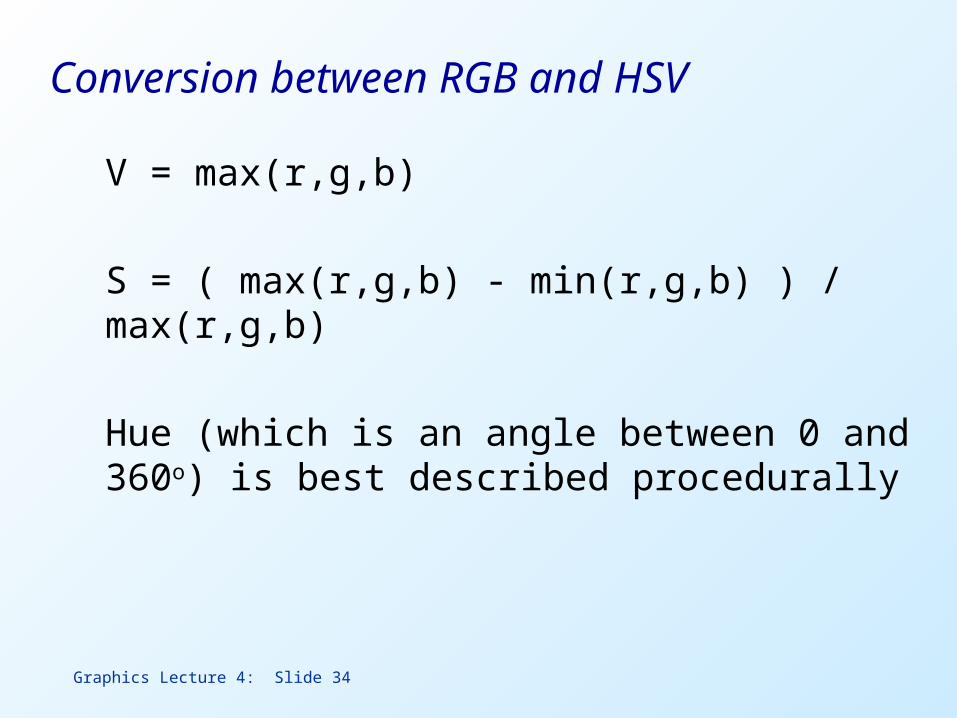
Conversion between RGB and HSV
V = max(r,g,b)
S = ( max(r,g,b) - min(r,g,b) ) / max(r,g,b)
Hue (which is an angle between 0 and 360o) is best described procedurally

Graphics Lecture 4: Slide 35
Calculating hue
if (r=g=b) Hue is undefined, the colour is black, white or grey.
if (r>b) and (g>b) Hue = 120*(g-b)/((r-b)+(g-b))
if (g>r) and (b>r) Hue = 120 + 120*(b-r)/((g-r)+(b-r))
if (r>g) and (b>g) Hue = 240 +120*(r-g)/((r-g)+(b-g))
Graphics Lecture 4: Slide 36
Saturation in the RGB system
In the RGB system we can treat each point as a mixture of pure colour and white.
Note however that the so called pure colours are not coherent wavelengths as in the CIE diagram
Graphics Lecture 4: Slide 37
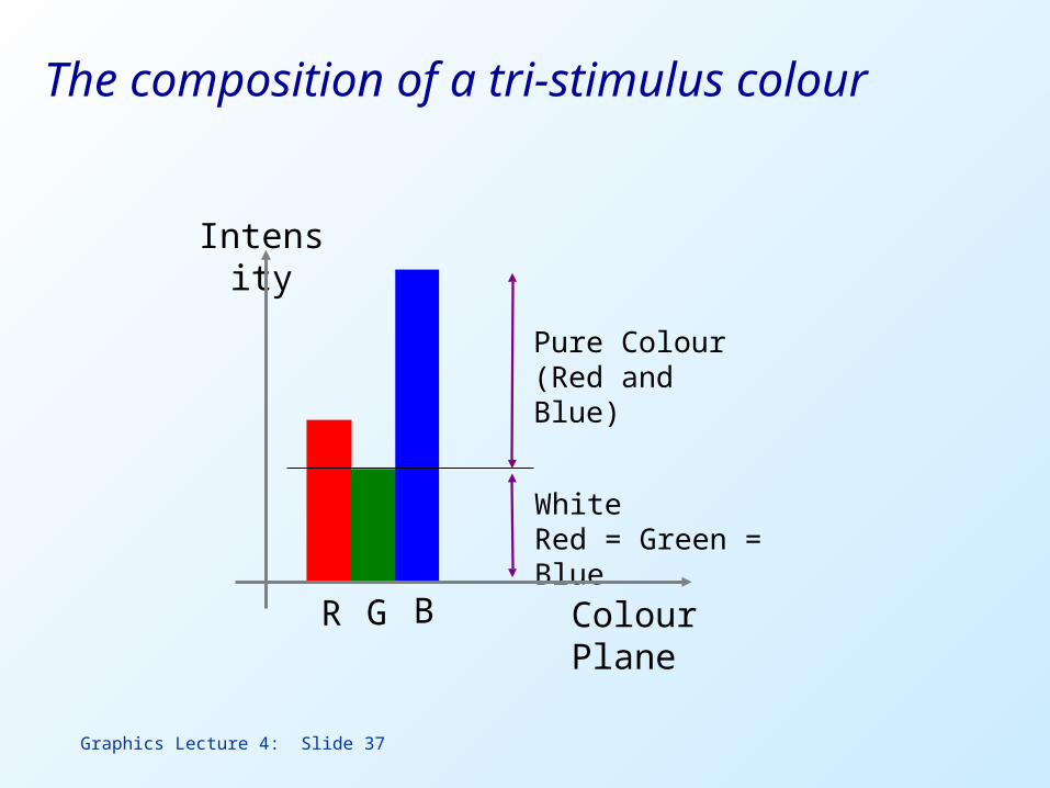
R
Intensity
Colour PlaneG B
Pure Colour (Red and Blue)
White Red = Green = Blue
The composition of a tri-stimulus colour
Graphics Lecture 4: Slide 38
Alpha Channels
Colour representations in computer systems sometimes use four components - r g b .
The fourth is simply an attenuation of the intensity which:
allows greater flexibility in representing colours.
avoids truncation errors at low intensity
allows convenient masking certain parts of an image.