Embed Size (px)
Citation preview
Interactive Graphics Lecture 9: Slide 1
Interactive Graphics
Lecture 9: Introduction to Spline Curves
Interactive Graphics Lecture 13: Slide 2
Interactive Graphics Lecture 9: Slide 3
Splines
The word spline comes from the ship building trade where planks were originally shaped by bending them round pegs fixed in the ground.
Originally it was the pegs that were referred to as splines.
Now it is the smooth curve that is called a spline.
Interactive Graphics Lecture 9: Slide 4
Interpolating Splines
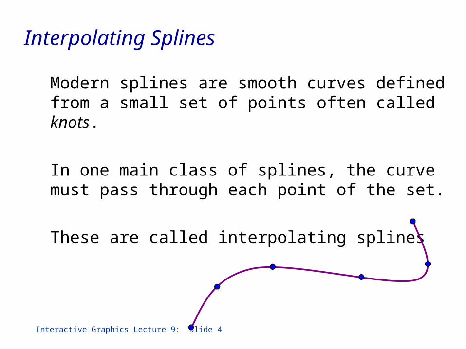
Modern splines are smooth curves defined from a small set of points often called knots.
In one main class of splines, the curve must pass through each point of the set.
These are called interpolating splines
Interactive Graphics Lecture 9: Slide 5
Approximating Splines
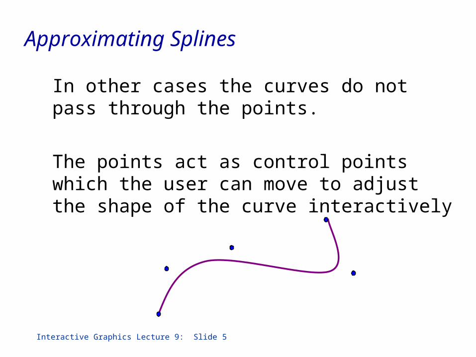
In other cases the curves do not pass through the points.
The points act as control points which the user can move to adjust the shape of the curve interactively
Interactive Graphics Lecture 9: Slide 6
Non Parametric Spline
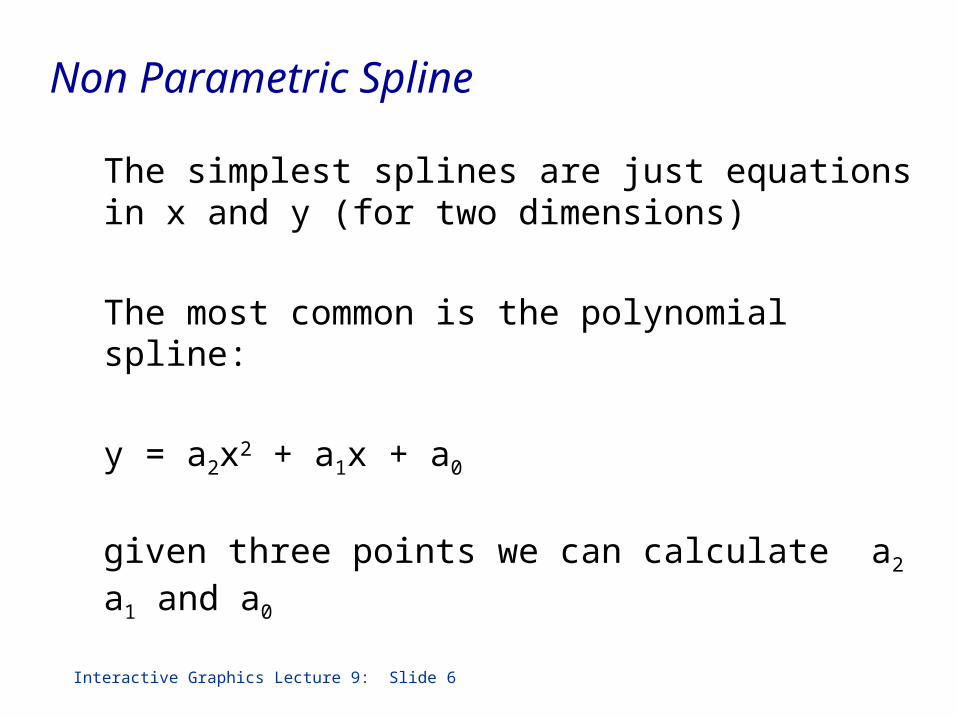
The simplest splines are just equations in x and y (for two dimensions)
The most common is the polynomial spline:
y = a2x2 + a1x + a0
given three points we can calculate a2 a1 and a0
Interactive Graphics Lecture 9: Slide 7
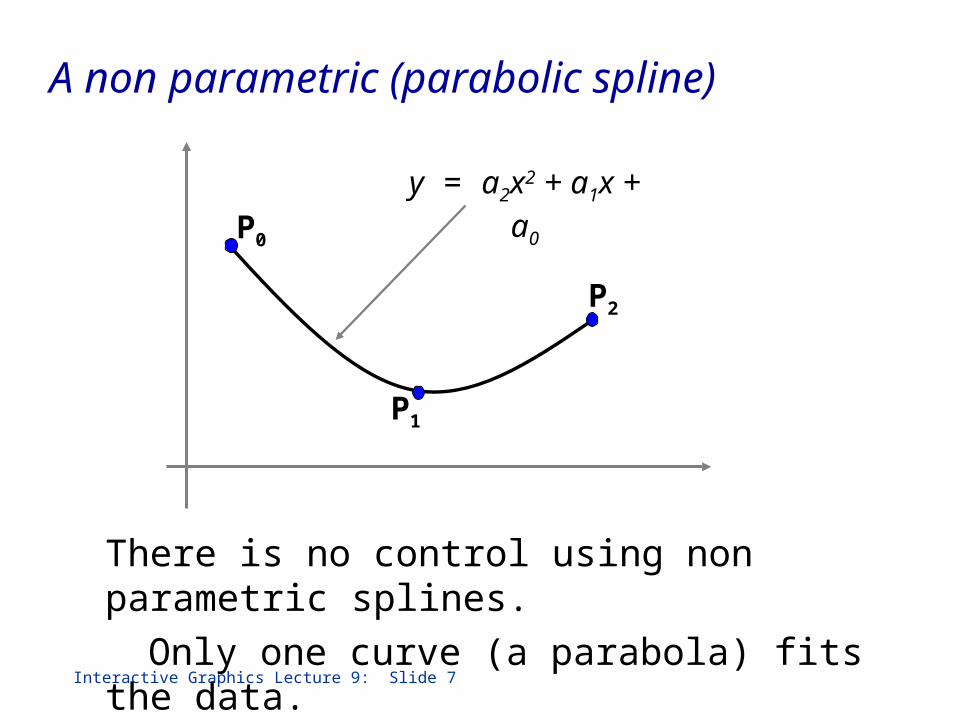
A non parametric (parabolic spline)
P0
P1
P2
y = a2x2 + a1x + a0
There is no control using non parametric splines.
Only one curve (a parabola) fits the data.
Interactive Graphics Lecture 9: Slide 8
Parametric Splines
If we write our spline in a vector form we get:
P = a22 + a1 + a0
which has a parameter
by convention, as ranges from 0 to 1 the point P traces out a curve.
Interactive Graphics Lecture 9: Slide 9
Calculating simple parametric splines
We can now solve for the vector constants a0 a1 and a2 as follows.
Suppose we want the curve to start at point P0
P0 = a22 + a1 + a0
we have =0 at the start so
P0 = a0
Interactive Graphics Lecture 9: Slide 10
Calculating simple parametric splines
Suppose we want the spline to end at P2
we have that at the end = 1
thus P2 = a22 + a1 + a0
= a2 + a1 + a0
= a2 + a1 + P0
Interactive Graphics Lecture 9: Slide 11
Calculating simple parametric splines
and in the middle (say = 1/2) we want it to pass through P1
P1 = a22 + a1 + a0
= a2 + a1 + P0
We have enough equations to solve for a1 and a2.
Notice that this formulation is the same in 2 and 3 dimensions.
Interactive Graphics Lecture 9: Slide 12
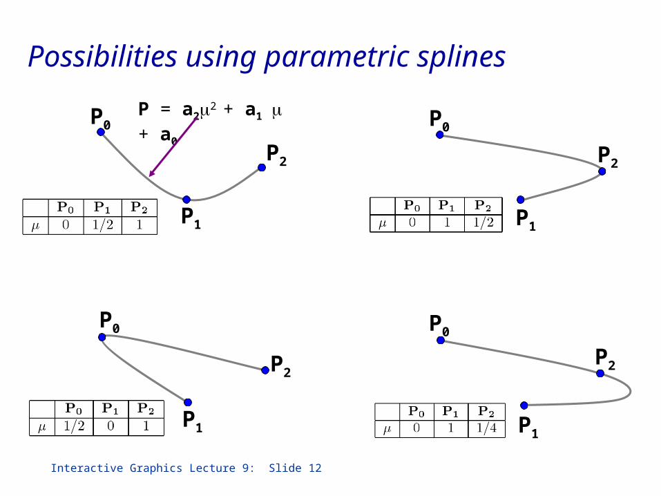
Possibilities using parametric splines
P0
P1
P2
P0
P1
P2
P = a22 + a1 + a0 P0
P1
P2
P0
P1
P2
Interactive Graphics Lecture 9: Slide 13
Higher order parametric splines
Parametric polynomial splines must have an order to match the number of knots.
3 knots - quadratic polynomial 4 knots - cubic polynomial etc.
Higher order polynomials are undesirable since they tend to oscillate
Interactive Graphics Lecture 9: Slide 14
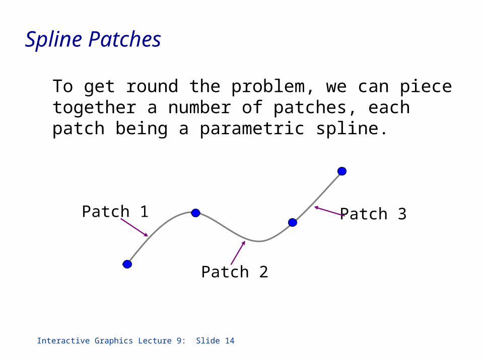
Spline Patches
To get round the problem, we can piece together a number of patches, each patch being a parametric spline.
Patch 1 Patch 3
Patch 2
Interactive Graphics Lecture 9: Slide 15
Cubic Spline Patches
The simplest, and most effective way to calculate parametric spline patches is to use a cubic polynomial.
P = a33 + a22 + a1 + a0
This allows us to join the patches together smoothly
Interactive Graphics Lecture 9: Slide 16
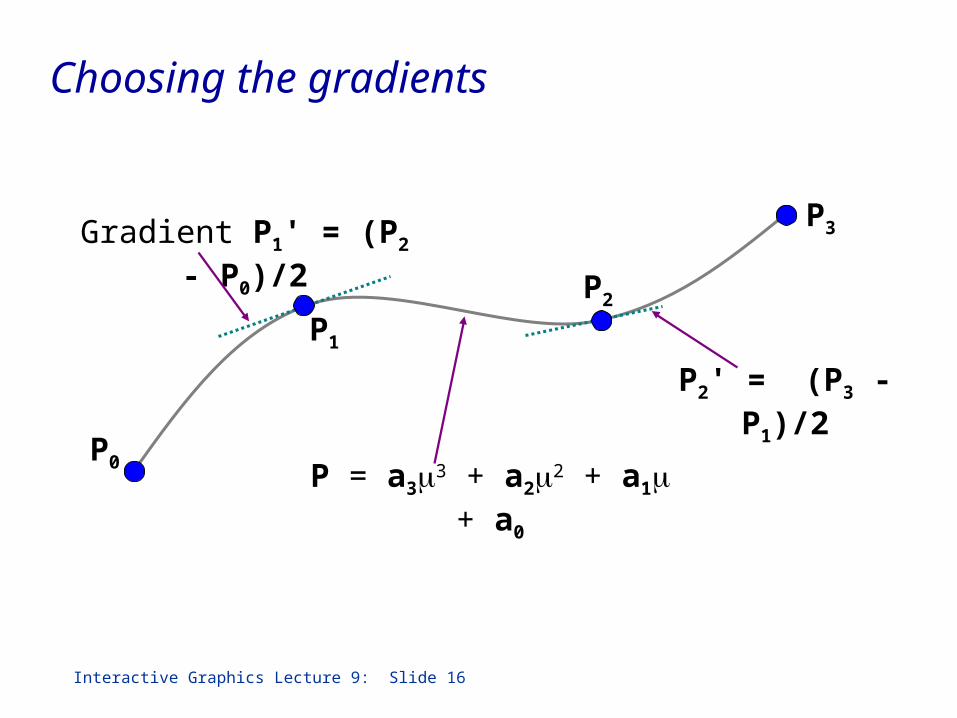
Choosing the gradients
P = a33 + a22 + a1 + a0
P0
P3
P1
P2
Gradient P1' = (P2 - P0)/2
P2' = (P3 - P1)/2
Interactive Graphics Lecture 9: Slide 17
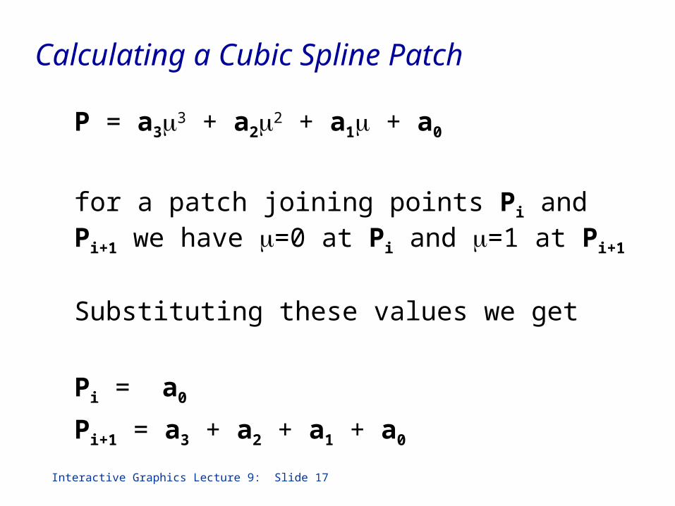
Calculating a Cubic Spline Patch
P = a33 + a22 + a1 + a0
for a patch joining points Pi and Pi+1 we have =0 at Pi and =1 at Pi+1
Substituting these values we get
Pi = a0
Pi+1 = a3 + a2 + a1 + a0
Interactive Graphics Lecture 9: Slide 18
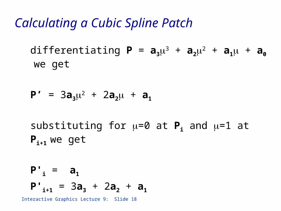
Calculating a Cubic Spline Patch
differentiating P = a33 + a22 + a1 + a0 we get
P’ = 3a32 + 2a2 + a1
substituting for =0 at Pi and =1 at Pi+1 we get
P'i = a1
P'i+1 = 3a3 + 2a2 + a1
Interactive Graphics Lecture 9: Slide 19
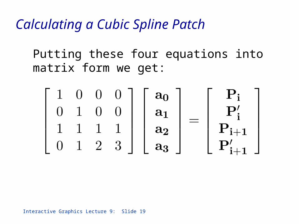
Calculating a Cubic Spline Patch
Putting these four equations into matrix form we get:
Interactive Graphics Lecture 9: Slide 20
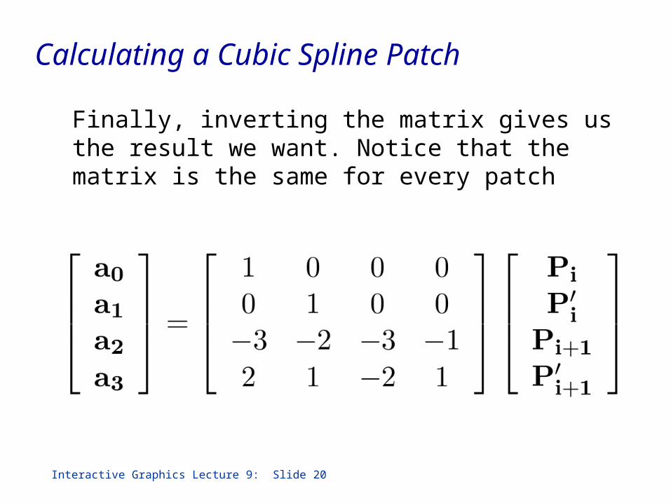
Calculating a Cubic Spline Patch
Finally, inverting the matrix gives us the result we want. Notice that the matrix is the same for every patch
Interactive Graphics Lecture 9: Slide 21
Bezier Curves
Bezier curves were developed as a method for CAD design. They give very predictable results for small sets of knots, and so are useful as spline patches.
The main characteristics of Bezier curves are
They interpolate the end points
The slope at an end is the same as the line joining the end point to its neighbour
Interactive Graphics Lecture 9: Slide 22
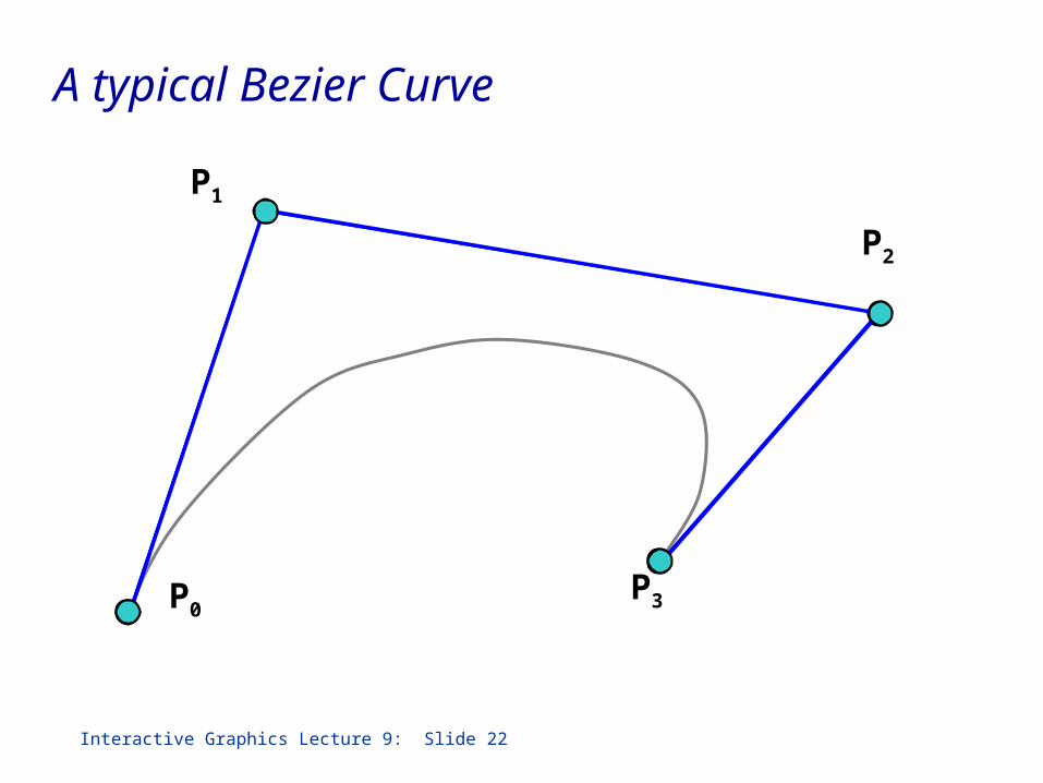
A typical Bezier Curve
P0P3
P2
P1
Interactive Graphics Lecture 9: Slide 23
Casteljau’s Algorithm
Bezier curves may be computed and visualised using a geometric construction due to Paul de Casteljau.
Like a cubic patch, we need a parameter which is to be 0 at the start of the curve, and 1 at the end.
A construction can be made for any value of
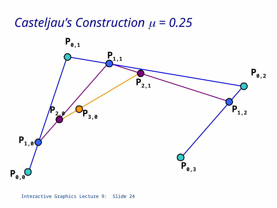
Interactive Graphics Lecture 9: Slide 24
P0,0
P0,3
P0,2
P0,1
P3,0P2,0
P2,1
P1,0
P1,1
P1,2
Casteljau’s Construction = 0.25
Interactive Graphics Lecture 9: Slide 25
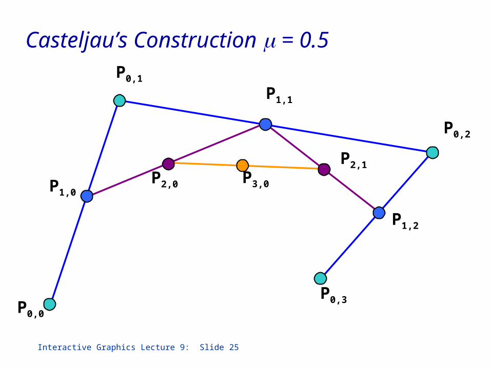
Casteljau’s Construction = 0.5
P0,0
P0,3
P0,2
P0,1
P3,0P2,0
P2,1
P1,0
P1,1
P1,2
Interactive Graphics Lecture 9: Slide 26
P0,0
P0,3
P0,2
P0,1
P3,0
P2,0
P2,1
P1,0
P1,1
P1,2
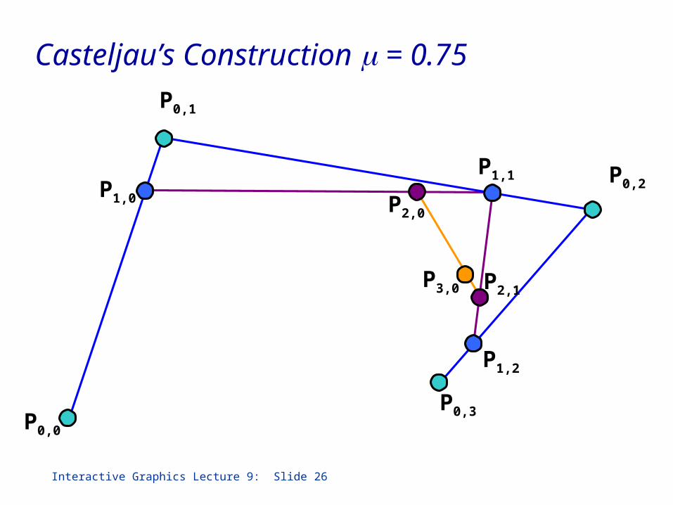
Casteljau’s Construction = 0.75
Interactive Graphics Lecture 9: Slide 27
Bernstein Blending Function
Splines (including Bezier curves) can be formulated as a blend of the knots.
Consider the vector line equation
P = (1-)P0 + P1
It is a linear ‘blend’ of two points, and could also be considered the 2 point Bezier curve!
Interactive Graphics Lecture 9: Slide 28
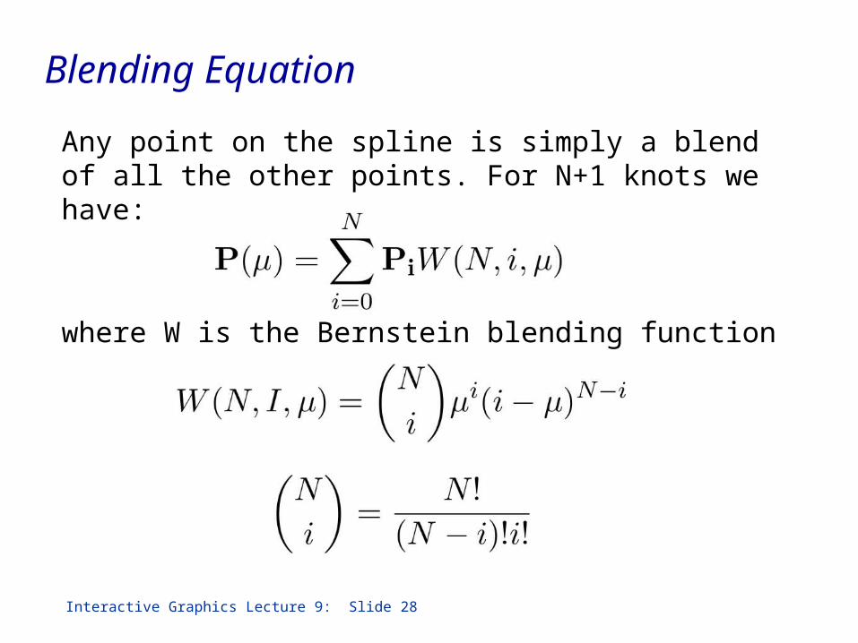
Blending Equation
Any point on the spline is simply a blend of all the other points. For N+1 knots we have:
where W is the Bernstein blending function
Interactive Graphics Lecture 9: Slide 29
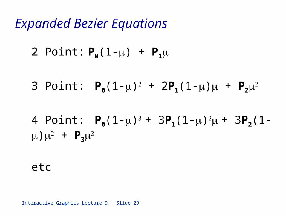
Expanded Bezier Equations
2 Point: P0(1-) + P1
3 Point: P0(1-)+ 2P1(1-) + P2
4 Point: P0(1-)+ 3P1(1-)+ 3P2(1-) + P3
etc
Interactive Graphics Lecture 9: Slide 30
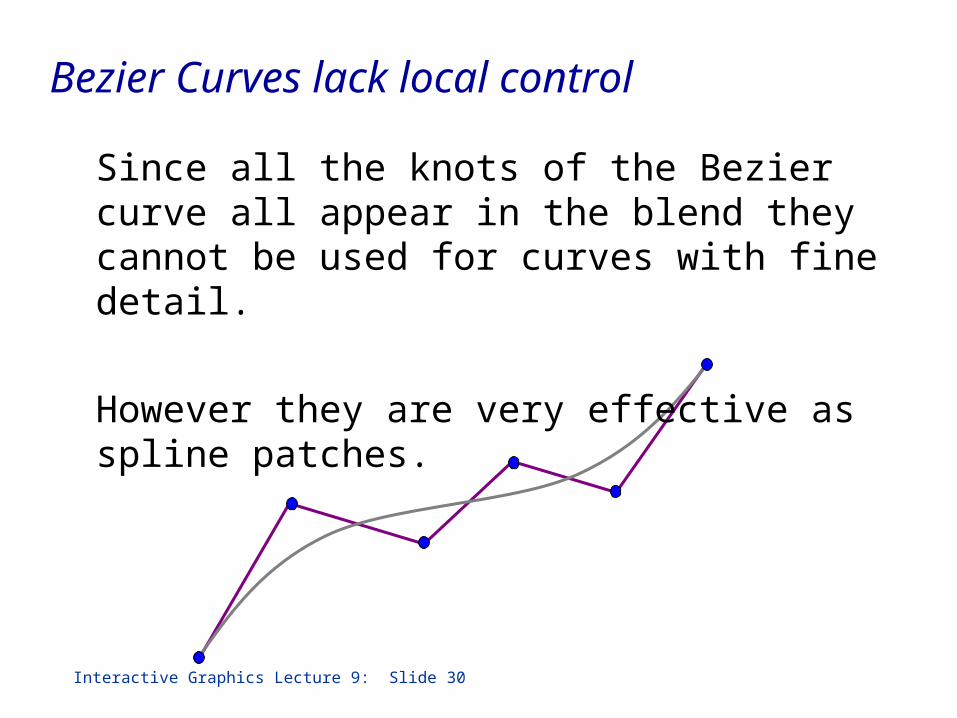
Bezier Curves lack local control
Since all the knots of the Bezier curve all appear in the blend they cannot be used for curves with fine detail.
However they are very effective as spline patches.
Interactive Graphics Lecture 9: Slide 31
Four point Bezier Curves and Cubic Patches
Four point Bezier curves are equivalent to cubic patches going through the first and last knot (P0 and P3)
It is possible to show their equivalence in two ways:
Expanding the iterative blending equation Reversing the de Casteljau algorithm
Interactive Graphics Lecture 9: Slide 32
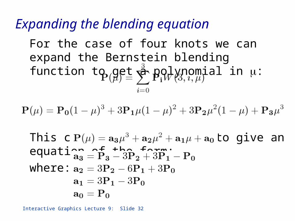
Expanding the blending equation
For the case of four knots we can expand the Bernstein blending function to get a polynomial in :
This can be multiplied out to give an equation of the form:
where:
Interactive Graphics Lecture 9: Slide 33
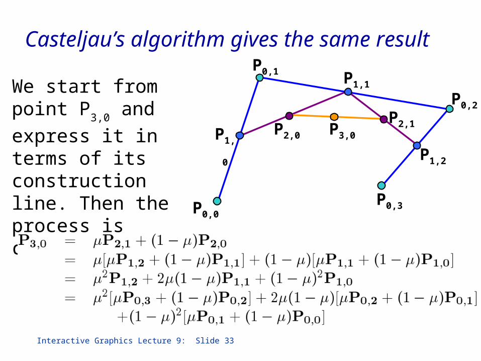
Casteljau’s algorithm gives the same result
P0,0P0,3
P0,2
P0,1
P3,0P2,0
P2,1P1,0
P1,1
P1,2
We start from point P3,0
and express it in terms of its construction line. Then the process is continued.
Interactive Graphics Lecture 9: Slide 34
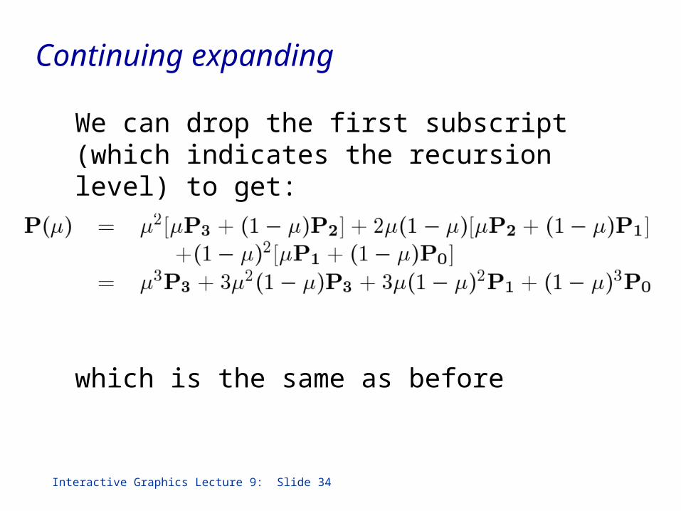
Continuing expanding
We can drop the first subscript (which indicates the recursion level) to get:
which is the same as before
Interactive Graphics Lecture 9: Slide 35
Control Points
We can summarise the four point Bezier Curve by saying that it has two points that are interpolated and two control points.
The curve starts at P0 and ends at P3 and its shape can be determined by moving control points (P1 and P2).
This could be done interactively using a mouse.
Interactive Graphics Lecture 9: Slide 36
In summary
The simplest and most effective way to draw a smooth curve through a set of points is to use a cubic patch.
If no interaction is needed setting the gradients by the central difference (Pi+1 - Pi-1)/2 is effective.
If the user wants to interactively adjust the shape the four point Bezier formulation is ideal