Embed Size (px)
Citation preview
Uncertainty analysis ofPhast’s atmospheric dispersion model
for two industrial use cases
Nishant Pandya, Nadine Gabas & Eric Marsden
Loss Prevention 2013, Firenze
Context
. Postdoctoral work of Nishant Pandya• Toulouse Chemical Engineering laboratory (CNRS)• Foundation for an Industrial Safety Culture• industrial partners including DNV Software
. Simulation of atmospheric dispersion of gas releases• complex physical phenomena• often dimensioning scenarios for land-use planning
. Phast is widely used to analyze these release scenarios• modeling involves a large number of variables and parameters• variables and parameters affected by uncertainty
. Political pressure to improve characterization of uncertainty inmodelling results
• new French legislation on land-use planning around Seveso-typeinstallations
2 / 18 Loss Prevention 2013
Study objectives
. Uncertainty analysis of Phast version 6.7• leak source term• outdoor dispersion model
. Analyze 10–30 minute continuous releases of four materials• two toxic (ammonia, nitric oxide)• two flammable (methane, propane)
. Examine the impact of representative variations of physical variables& internal model parameters
• uncertainty propagation
. Two different use-cases:• accident-investigation• risk-prevention
3 / 18 Loss Prevention 2013
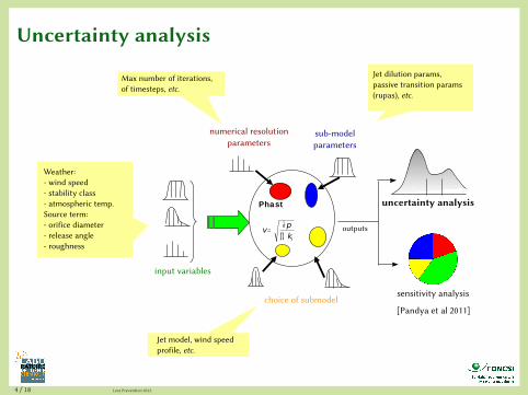
Uncertainty analysis
choice of submodel
Phast
numerical resolutionparameters
input variables
sub-modelparameters
uncertainty analysis
sensitivity analysis
[Pandya et al 2011]
outputsikp
v∏∂=
Max number of iterations,of timesteps, etc.
Jet model, wind speed profile, etc.
Weather: - wind speed- stability class- atmospheric temp.Source term:- orifice diameter- release angle- roughness
Jet dilution params, passive transition params(rupas), etc.
4 / 18 Loss Prevention 2013
Uncertainty analysis
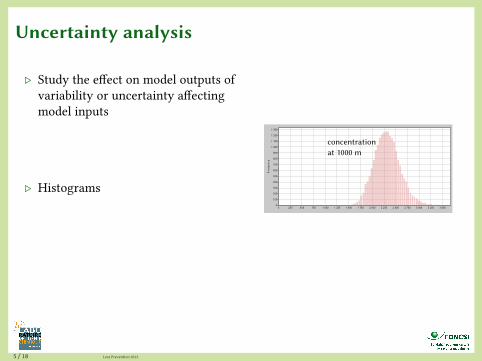
. Study the effect on model outputs ofvariability or uncertainty affectingmodel inputs
. Histograms
. Quantified using the coefficient ofvariation
• CV =σ
µ
5 / 18 Loss Prevention 2013
Uncertainty analysis
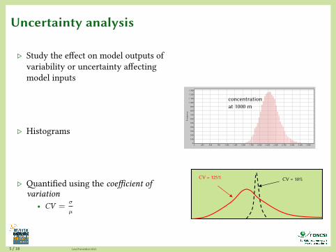
. Study the effect on model outputs ofvariability or uncertainty affectingmodel inputs
. Histograms
. Quantified using the coefficient ofvariation
• CV =σ
µ
concentrationat 1000 m
5 / 18 Loss Prevention 2013
Uncertainty analysis
. Study the effect on model outputs ofvariability or uncertainty affectingmodel inputs
. Histograms
. Quantified using the coefficient ofvariation
• CV =σ
µ
concentrationat 1000 m
CV = 10%CV = 125%
5 / 18 Loss Prevention 2013
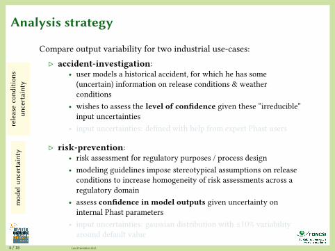
Analysis strategy
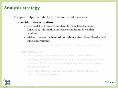
Compare output variability for two industrial use-cases:. accident-investigation:
• user models a historical accident, for which he has some(uncertain) information on release conditions & weatherconditions
• wishes to assess the level of confidence given these “irreducible”input uncertainties
• input uncertainties: defined with help from expert Phast users
. risk-prevention:• risk assessment for regulatory purposes / process design• modeling guidelines impose stereotypical assumptions on releaseconditions to increase homogeneity of risk assessments across aregulatory domain
• assess confidence in model outputs given uncertainty oninternal Phast parameters
• input uncertainties: gaussian distribution with ±10% variabilityaround default value
6 / 18 Loss Prevention 2013
Analysis strategy
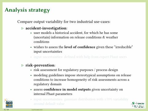
Compare output variability for two industrial use-cases:. accident-investigation:
• user models a historical accident, for which he has some(uncertain) information on release conditions & weatherconditions
• wishes to assess the level of confidence given these “irreducible”input uncertainties
• input uncertainties: defined with help from expert Phast users
. risk-prevention:• risk assessment for regulatory purposes / process design• modeling guidelines impose stereotypical assumptions on releaseconditions to increase homogeneity of risk assessments across aregulatory domain
• assess confidence in model outputs given uncertainty oninternal Phast parameters
• input uncertainties: gaussian distribution with ±10% variabilityaround default value
6 / 18 Loss Prevention 2013
Analysis strategy
Compare output variability for two industrial use-cases:. accident-investigation:
• user models a historical accident, for which he has some(uncertain) information on release conditions & weatherconditions
• wishes to assess the level of confidence given these “irreducible”input uncertainties
• input uncertainties: defined with help from expert Phast users
. risk-prevention:• risk assessment for regulatory purposes / process design• modeling guidelines impose stereotypical assumptions on releaseconditions to increase homogeneity of risk assessments across aregulatory domain
• assess confidence in model outputs given uncertainty oninternal Phast parameters
• input uncertainties: gaussian distribution with ±10% variabilityaround default value
releasecond
itions
uncertainty
mod
elun
certainty
6 / 18 Loss Prevention 2013
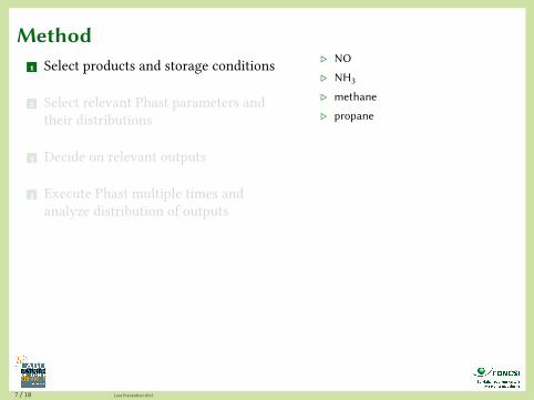
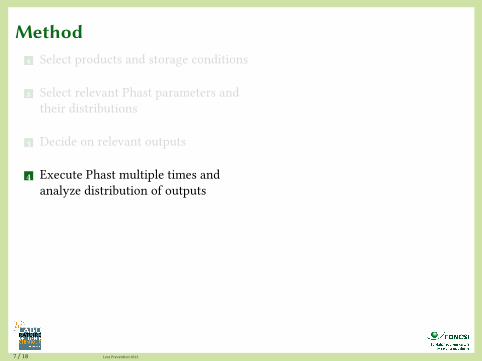
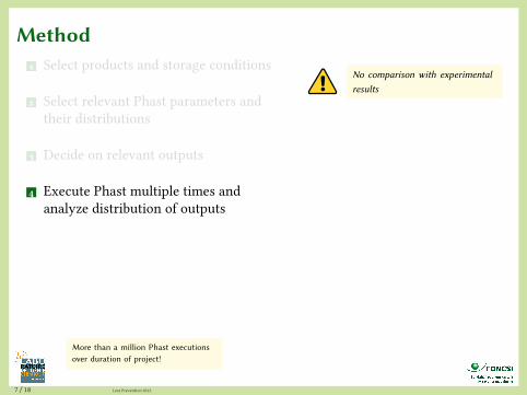
Method1 Select products and storage conditions
2 Select relevant Phast parameters andtheir distributions
3 Decide on relevant outputs
4 Execute Phast multiple times andanalyze distribution of outputs
. NO
. NH3
. methane
. propane
7 / 18 Loss Prevention 2013
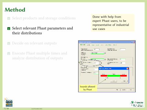
Method1 Select products and storage conditions
2 Select relevant Phast parameters andtheir distributions
3 Decide on relevant outputs
4 Execute Phast multiple times andanalyze distribution of outputs
Done with help fromexpert Phast users, to berepresentative of industrialuse cases
bounds allowedby Phast
7 / 18 Loss Prevention 2013
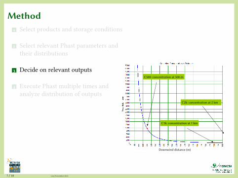
Method1 Select products and storage conditions
2 Select relevant Phast parameters andtheir distributions
3 Decide on relevant outputs
4 Execute Phast multiple times andanalyze distribution of outputs
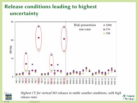
12
C500: concentration at 500 m
C1k: concentration at 1 km
C2k: concentration at 2 km
Downwind distance (m)
7 / 18 Loss Prevention 2013
Method1 Select products and storage conditions
2 Select relevant Phast parameters andtheir distributions
3 Decide on relevant outputs
4 Execute Phast multiple times andanalyze distribution of outputs
7 / 18 Loss Prevention 2013
Method1 Select products and storage conditions
2 Select relevant Phast parameters andtheir distributions
3 Decide on relevant outputs
4 Execute Phast multiple times andanalyze distribution of outputs
No comparison with experimentalresults
More than a million Phast executionsover duration of project!
7 / 18 Loss Prevention 2013

Scenario tree: risk-prevention use-case
. Fine-grained scenario-based approach facilitates interpretation of results
. 4 “bifurcation parameters”: release duration, release rate, weatherconditions, release angle→ 16 scenarios
θ 0°
10 min. duration 30 min. duration
continuous release
low release rate high release rate
θ 90°
neutralweather
stableweather
θ 0° θ 90°
Sc 3 Sc 4
θ 0° θ 90°
Sc 5
θ 0° θ 90°
Sc 6 Sc 7 Sc 8
θ 0° θ 90°
Sc 9
θ 0° θ 90°
Sc 10 Sc 11 Sc 12
θ 0° θ 90°
Sc 13
θ 0° θ 90°
Sc 14 Sc 15 Sc 16Sc 1 Sc 2
high release ratelow release rate
neutralweather
neutralweather
neutralweather
stableweather
stableweather
stableweather
“Low” and “high” release rates selected to be product-appropriate8 / 18 Loss Prevention 2013
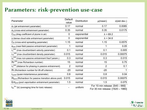
Parameters: risk-prevention use-case
Parameter Default value
Distribution µ(mean) σ(std dev.)
α1 (jet entrainment parameter) 0.17 normal 0.17 0.0085
α2 (cross-wind entrainment parameter) 0.35 normal 0.35 0.0175
CDa (drag coefficient of plume in air) 0 exponential λ = 69.2
γ (dense cloud side entrainment parameter) 0 exponential λ = 34.6
CE (cross-wind spreading parameter) 1.15 normal 1.15 0.0575
epas (near-field passive entrainment parameter) 1 normal 1 0.05
rupas
(max cloud/ambient velocity parameter) 0.1 normal 0.1 0.005
rropas
(max cloud/ambient density parameter) 0.015 normal 0.015 0.00075
rEpas
(max non-passive entrainment fract° param.) 0.3 normal 0.3 0.015
Ri*pas
(max Richardson number) 15 normal 15 0.75
rtrpas
(distance for phasing in passive entrainment) 2 normal 2 0.1
Ri (Richardson number for lift-off criterion) -20 normal -20 1
rquasi (quasi-instantaneous parameter) 0.8 normal 0.8 0.04
Ripool (Richardson for passive transition above pool) 0.015 normal 0.015 0.00075
Entpool (pool vaporisation entrainment parameter) 1.5 normal 1.5 0.075
tavtox (s) (averaging time for toxic release) - uniform
For 10 min release: [540 – 660] For 30 min release: [1620 – 1980]
9 / 18 Loss Prevention 2013
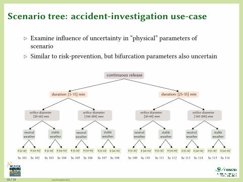
Scenario tree: accident-investigation use-case
. Examine influence of uncertainty in “physical” parameters ofscenario
. Similar to risk-prevention, but bifurcation parameters also uncertain
duration: [5-15] min duration: [25-35] min
continuous release
orifice diameter[20-60] mm
orifice diameter[160-200] mm
θ [0-30]° θ [60-90]°
orifice diameter[20-60] mm
orifice diameter[160-200] mm
neutralweather
stableweather
Sc 103 Sc 104 Sc 105 Sc 106 Sc 107 Sc 108 Sc 109 Sc 110 Sc 111 Sc 112 Sc 113 Sc 114 Sc 115 Sc 116Sc 101 Sc 102
neutralweather
neutralweather
neutralweather
stableweather
stableweather
stableweather
θ [0-30]° θ [0-30]° θ [0-30]°θ [60-90]° θ [60-90]° θ [60-90]° θ [0-30]° θ [0-30]° θ [0-30]°θ [0-30]°θ [60-90]° θ [60-90]° θ [60-90]° θ [60-90]°
10 / 18 Loss Prevention 2013

Parameters: accident-investigation use-case
Parameter Nomenclature / Unit Distribution Range of variation
Tst Storage temperature / K triangular NH3: [263.15 – 283.15] centered at 273.15 K
NO, CH4, C3H8: [273.15-293.15] centered at 283.1K
Lh Liquid height / m uniform [12.75 - 17.25]
Ta Atmospheric temperature / K triangular [282.65 - 287.65] centered at 285.15 K
Pa Atmospheric pressure / Pa uniform [0.99·105 - 1.035·105]
Ha Relative atmospheric humidity / - triangular [0.55 - 0.85] centered at 0.7
DO Orifice diameter / m triangular Value 1: [0.02 - 0.06] centered at 0.04 Value 2: [0.16 - 0.20] centered at 0.18
Durmax Maximum release duration / s uniform Value 1: [300 - 900] Value 2: [1500 - 2100]
angle Release angle / degree uniform Value 1: [0 - 30] Value 2: [60 - 90]
SC Stability Class / - discrete Neutral: [10 % C/D, 80 % D, 10 % E]
Stable: [10 % E, 80 % F, 10 % G]
ua Wind speed / m·s-1 uniform Neutral: [4 - 6] Stable: [1.5 - 3]
Sflux Solar radiation flux / W·m-2 triangular Neutral: [250 - 1000] centered at 500
Stable: [0 - 500] centered at 250
ZR Release height above ground/ m uniform [1 - 10]
Z0 Surface roughness length / m triangular [0.5 - 1.5] centered at 1 m
11 / 18 Loss Prevention 2013
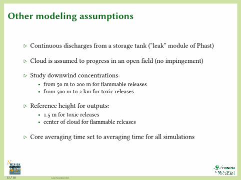
Other modeling assumptions
. Continuous discharges from a storage tank (“leak” module of Phast)
. Cloud is assumed to progress in an open field (no impingement)
. Study downwind concentrations:• from 50 m to 200 m for flammable releases• from 500 m to 2 km for toxic releases
. Reference height for outputs:• 1.5 m for toxic releases• center of cloud for flammable releases
. Core averaging time set to averaging time for all simulations
12 / 18 Loss Prevention 2013
Three types of results
1 Scenario-specific uncertainty information fordecision-makers
2 Comparing uncertainty for two industrial use-cases
3 Identify release conditions which lead to the highest levelof uncertainty
13 / 18 Loss Prevention 2013
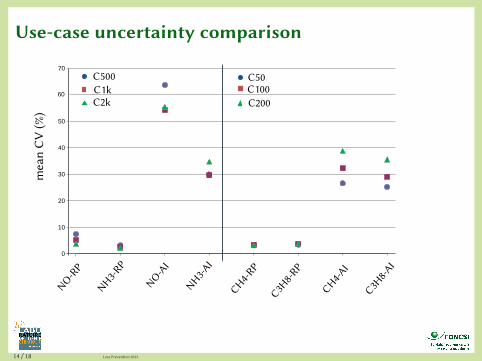
Use-case uncertainty comparisonm
ean
CV
(%)
NO-RP
NH3-RP
NO-AI
NH3-AI
CH4-RP
C3H8-
RP
CH4-AI
C3H8-A
I
C200C100C50C500
C1kC2k
As expected, level of uncertainty always higher for “accident-investigation”than for “risk-prevention” use-cases
14 / 18 Loss Prevention 2013
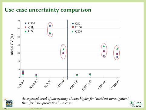
Use-case uncertainty comparisonm
ean
CV
(%)
NO-RP
NH3-RP
NO-AI
NH3-AI
CH4-RP
C3H8-
RP
CH4-AI
C3H8-A
I
C200C100C50C500
C1kC2k
As expected, level of uncertainty always higher for “accident-investigation”than for “risk-prevention” use-cases
14 / 18 Loss Prevention 2013

Release conditions leading to highestuncertainty
Risk-prevention use-case
Highest CV for vertical NO releases in stable weather conditions, with highrelease rates
15 / 18 Loss Prevention 2013
Release conditions leading to highestuncertainty
Risk-prevention use-case
Highest CV for vertical NO releases in stable weather conditions, with highrelease rates
15 / 18 Loss Prevention 2013
Conclusions
16 / 18 Loss Prevention 2013

Conclusions
. For the 4 materials studied, model uncertainty is significantly lowerthan uncertainty resulting from variation in source term and weatherconditions
. We have identified the release conditions which lead to the highestlevel of model uncertainty (material-dependent)
. Quantitative information on level of uncertainty in consequenceestimations:
• helps risk analysts understand the degree of confidence they can placein modeling results
• when comparing risk reduction measures, tells whether investmentranking is robust, given modeling uncertainties
• when modeling results inform land-use planning, provides informationwhich can help arbitrate between different strategies
. All modeling results presented to decision-makers should ideallyinclude information on level of uncertainty
17 / 18 Loss Prevention 2013
Thanks for your attention!
Follow the FonCSI on Twitter: @TheFonCSIThis presentation is distributed under theterms of the Creative Commons Attribution– ShareAlike licence.
18 / 18 Loss Prevention 2013