Top income shares and mortality: Evidence from advanced countries

257Top incomeshare andmortality:

Evidence fromadvancedcountries

Petri Böckerman

PALKANSAAJIEN TUTKIMUSLAITOS •TYÖPAPEREITA LABOUR INSTITUTE FOR ECONOMIC RESEARCH • DISCUSSION PAPERS

* Labour Institute for Economic Research and University of Tampere. Pitkänsillanranta 3A, 6. krs. FIN-00530 Helsinki, FINLAND.

Phone: +358-9-25357330. Fax: +358-9-25357332. E-mail: [email protected]

Helsinki 2010

257

Top income shares and mortality: Evidence from advanced countries

Petri Böckerman*

ISBN 978−952−209−076–8 ISSN 1795−1801

3

TIIVISTELMÄ

Tutkimuksessa tarkastellaan huipputulo-osuuksien vaikutusta kuolleisuuteen yhdeksän maan paneeli-

aineistolla vuosina 1952-1998. Tulosten mukaan huipputulojen osuudella ei ole yhteyttä kuolleisuu-

teen.

ABSTRACT

The paper examines the effect of top income shares on the crude death and infant mortality rates. We

use balanced panel data that covers nine advanced countries over the period 1952-1998. Top income

shares are measured as the shares of pre-tax income going to the richest 0.1%, 1% and 10% of the

population. We also estimate separate effects on both female and male mortality rates. The most

important finding is that there is no overall relationship between top income shares and mortality. If

anything, the estimates based on gender breakdown show that there is evidence that an increase in

income inequality is associated with a decrease in the crude death rate for males.

JEL Classification: I12; N30

KEY WORDS: income inequality; top income shares; mortality

1. INTRODUCTION

Increasing income inequality is said to be associated with increased morbidity and premature

mortality (see Wilkinson, 1996; Wagstaff and van Doorslaer, 2000; Subramanian and Kawachi, 2004;

Wilkinson and Pickett, 2006; Leigh et al., 2009, for surveys). However, the robustness of this

relationship has been questioned (e.g. Judge et al., 1998; Deaton, 2001; Gravelle et al., 2001; Deaton

and Lubotsky, 2003; Gerdtham and Johannesson, 2004; Lorgelly and Lindley, 2008). Most of the

literature has used cross-sectional data sets that do not allow controlling for unobservable

heterogeneity that is associated with regions/countries and years. In contrast, by using panel data on

countries it is possible to hold constant both stable country-to-country differences and annual changes

in the outcome of interest that affect all countries similarly in the same year (Leigh and Jencks, 2007).

There are earlier studies on income inequality and various domains of health that have used a panel

4

data approach, but they typically rely on a relatively short time dimension (e.g. Gravelle and Sutton,

2008; Kravdal, 2008; Hildebrand and Van Kerm, 2009).1

The paper examines the effect of top income shares on the crude death and infant mortality rates. We

use balanced panel data that covers nine advanced countries over the period 1952-1998. The most

important advantage of the measures of top income shares from tax registers is that they are available

for a much longer time period than other measures of income inequality. There is earlier research that

has used the measures of top income shares to examine the effect of income inequality on mortality

(Waldmann, 1992; Leigh and Jencks, 2007). Our paper differs from earlier research that has used

income tax data. First, we use three different measures of top income shares. These are the shares of

pre-tax income going to the richest 0.1%, 1% and 10% of the population.2 This is a crucial extension

of the literature, because the use of several different measures of top income shares allows us to detect

whether there exists a systematic, robust relationship between top income shares and mortality.

Second, we estimate separate effects on both female and male mortality rates. This is important,

because the overall effects can mask different effects on the mortality rates by gender. It is

particularly interesting to explore the potential gender differences in the relationship between income

inequality and mortality, because experimental evidence points out that gender differences exist in the

perception of equality and fairness (e.g. Eckel and Grossman, 2008). Females are generally more

sensitive to deviations from equality and fairness than males are. This implies that income inequality

may have stronger negative effects on females’ health. Third, we perform some robustness checks of

the relationship that have not been considered in this particular strand of research earlier. This is

essential, because the patterns that are based on the use of country aggregates on income inequality

and mortality can be fragile, at least to some degree. Lastly, we use a balanced panel from nine

advanced countries for the period 1952-1998. Thus, we do not use the pre-Second World War

observations on top income shares, because they often contain more measurement error (see e.g.

Roine et al., 2009). Neither do we use observations that cover the period of the Second World War,

because the shock of war may have had different idiosyncratic effects on the advanced countries that

are difficult to control for. Furthermore, it is useful to note that the parameters of interest are not

necessarily stable over the very long time period that would cover most of the twentieth century.

Because we focus on the analysis of a balanced panel, there is also no need to interpolate and/or

extrapolate for missing observations. This arguably reduces measurement error in the variables and

therefore produces more precise estimates with tighter confidence intervals.

1 Babones (2008) finds evidence for the positive relationship between income inequality and mortality by using panel data on countries over the period 1970-1995. 2 Leigh and Jencks (2007) use only the income share of the richest 10%.

5

2. DATA

We use data on mortality and top income shares for the period 1952-1998. The nine countries are the

following: Australia, Canada, France, Japan, New Zealand, Sweden, the Netherlands, the United

States and the United Kingdom. The time period and the countries have been selected in order to

construct a balanced panel of advanced countries.

The dependent variables of the models are based on the World Health Organization Mortality

Database.3 The database includes deaths by country from 1950, classified according to the

International Classification of Diseases System (ICD7-ICD10). In this paper, we use two measures of

mortality. These are the natural logarithm of the crude death rate (i.e. log of the total number of deaths

per year per 1000 inhabitants) and the natural logarithm of the infant mortality rate (i.e. log of the

number of deaths of children less than 1 year old per 1000 live births). Both measures of mortality are

also calculated separately for females and males by using the corresponding population shares.

The explanatory variables of interest are various measures of top income shares. Therefore, top

income shares are used as measures of income inequality. Collective research effort has constructed a

database on top income shares covering most of the twentieth century (Atkinson and Piketty, 2007;

2010).4 These measures are based on historical income tax statistics and common methodology across

countries.5 Top income shares are calculated by comparing the amount of income reported to the tax

authorities by the richest X% of individuals/households with an estimate of total personal income in

the same year from each country’s national accounts. In this paper, we use the shares of pre-tax

income going to the richest 0.1%, 1% and 10% of the population.6 Capital gains are not included in

the top income shares whenever they are separately reported, following Atkinson and Piketty (2010).

Piketty and Saez (2003:5-6) argue that capital gains should not be included in the top income shares,

because they are realized in a lumpy fashion. Hence, capital gains form a very volatile component of

income with a large variation from year to year. The income share of the richest 10% is not available

for Japan. Thus, the models that use the income share of the richest 10% are estimated for eight

advanced countries. As a control variable in the baseline specifications, we use the natural logarithm

3 The data are available at http://www.who.int/healthinfo/morttables/en/index.html 4 Piketty and Saez (2003) and Saez (2005) describe the trends in top income shares in the United States and Canada. 5 Atkinson and Brandolini (2001) discuss about the drawbacks of the commonly used “secondary” data sources on income inequality in detail. 6 The data on top income shares are described in Roine et al. (2009). The data that are used in the estimations are available at http://www.ifn.se/web/danielw.aspx

6

of the real GDP per capita (measured in 1990 international Geary-Khamis dollars), based on

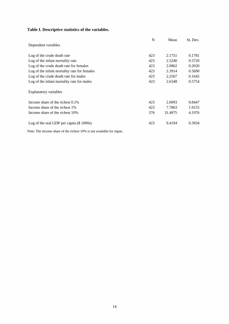
Maddison (2003).7 Table I provides descriptive statistics of the variables.

Table I here

3. EMPIRICAL APPROACH

We estimate models of the following type:

jttititiit GXY ελβα ++++= (1)

where Y is the outcome (log of the crude death rate or log of the infant mortality rate) for country i in

year t. X represents control variables. The variable of our interest is Git, which is a measure of top

income share for country i in year t. ε is an error term. iα and tλ represent fixed effects associated

with the country and the year. The most important advantage of the fixed effects approach is that we

are able to control for unobservable heterogeneity that is associated with countries and years.8 Thus,

in this fixed effects set-up, the effects of income inequality on mortality are identified by intra-

country variations, relative to the corresponding changes in other countries. Standard errors for the

estimates are clustered at the country level in all specifications to take into account the possible

within-country serial correlation, following Leigh and Jencks (2007).

7 The data are available at http://www.ggdc.net/maddison/ 8 Kravdal (2008:216-218) discusses about the fixed effects approach in detail. Böckerman et al. (2009) have also used the fixed effects approach to examine the relationship between income inequality and various subjective and objective measures of health.

7

4. RESULTS

4.1. Baseline estimates

We include the fixed effects for countries and years in the baseline specifications, because a full set of

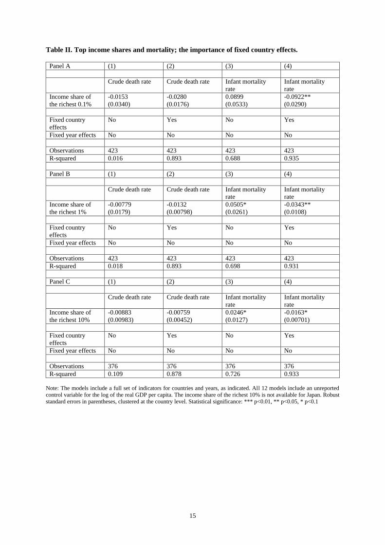
indicators for countries and years is statistically significant.9 For comparison, it is useful to note that

the point estimate of the income share of the richest 1% on the crude death rate is -0.0078 (with a

robust standard error of 0.0179, clustered at the country level) in the specification that does not

include a full set of indicators for countries (and years) (Table II, Panel B, Column 1). Even more

interestingly, the estimate of the income share of the richest 1% on the infant mortality rate is 0.0505

(0.0261) in the model without a full set of indicators for countries (and years) (Table II, Panel B,

Column 3). Therefore, the estimate suggests that an increase in income inequality increases infant

mortality. This result is in accordance with the cross-country estimates in Waldmann (1992) and the

specifications that do not include a full set of indicators for countries and years in Leigh and Jencks

(2007:11) and the cross-country correlations in Wilkinson and Pickett (2009:82). The most important

point regarding the appropriate model specification is that if the inclusion of the indicators for the

countries changes the estimate for income inequality, it means that the time-invariant unobserved

country characteristics are correlated with income inequality. This implies that a model specification

with a random term in order to capture unobserved country characteristics (or a simpler model

without such a term) would not be appropriate, because a model with a random term is based on the

assumption that the time-invariant unobserved country characteristics are not correlated with income

inequality, following the argument in Kravdal (2008:216-220). In our case the inclusion of a full set

of indicators for the countries (i.e. fixed country effects) clearly changes the estimates for income

inequality (Table II, Panels A-C, Columns 2 and 4). The change in the estimate for income inequality

is particularly significant for the infant mortality rate (Table II, Panels A-C, Columns 3-4). This

pattern prevails for all measures of top income shares. Thus, the fixed effects approach is the most

appropriate modelling approach in our case, based on the importance of fixed country effects.

Table II here

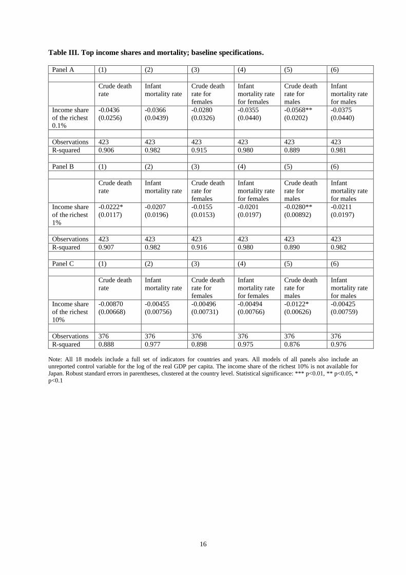
The most important finding from the baseline specifications is that there is no overall relationship

between top income shares and mortality among nine advanced countries over the period 1952-1998

(Table III, Panels A-C, Columns 1-2). The non-existence of a relationship between the income share

of the richest 10% and mortality is in accordance with the results in Leigh and Jencks (2007). Only in

9 Leigh and Jencks (2007:11) also find that the indicators for countries and years are highly statistically significant.

8

the specification that uses the share of income going to the richest 1% is there evidence of a negative

relationship at the 10% significance level between income inequality and the crude death rate (Table

III, Panel B, Column 1). For the infant mortality rate not even this relationship prevails. However, the

mortality rates that are calculated separately for females and males reveal an interesting additional

pattern. There is evidence that an increase in income inequality is associated with a decrease in the

crude death rate for males.10 This pattern prevails for all three measures of income inequality (Table

III, Panels A-C, Column 5). The 95% confidence intervals for these estimates indicate that zero is

generally not included in them. For example, the confidence intervals for the point estimate of the

income share of the richest 1% on the crude death rate for males (Table III, Panel B, Column 5) range

from -0.0485 to -0.0074. In contrast, for females there is no evidence whatsoever that income

inequality is related to mortality (Table III, Panels A-C, Columns 3-4).

Table III here

4.2. Robustness checks

To examine the robustness of the baseline estimates, we have estimated several additional

specifications.11 First, we have dropped one country at a time from the panel and re-estimated the

models. This allows us to detect whether the overall pattern in Table III is driven by the observations

that are related to one country only. None of these specifications indicates that there is evidence for

the positive relationship between top income shares and mortality. For example, the point estimates

for the income share of the richest 1% on the crude death rate (Table III, Panel B, Column 1) vary

from -0.0771 (with a robust standard error of 0.0211, clustered at the country level) to -0.0210

(0.0297) when one country at a time is dropped from the panel. We have also estimated separate

models for the Anglo-Saxon countries, because one of the best known stylized facts of the

development of top income shares is their diverging evolution in the Anglo-Saxon countries vs.

continental Europe (Atkinson and Piketty, 2007).12 The non-existence of the relationship between

income inequality and mortality remains. Second, we have estimated separate models for the periods

1950-1973 and 1973-1998, following the classification of growth phases in the advanced countries by

Maddison (1991). These results suggest that the relationship between top income shares and mortality

has changed over the period 1950-1998. In particular, there is evidence that a negative relationship

prevails over the period 1950-1973, but this relationship disappears over the period 1973-1998. For

10 Leigh and Jencks (2007) obtain some evidence for the positive coefficient for the income share of the richest 10% in the specifications for life expectancy at birth, but their estimates are generally not statistically significant. 11 The results of all robustness checks are available upon request. 12 We classify Australia, Canada, New Zealand, the UK, and the US as the Anglo-Saxon countries, following e.g. Roine et al. (2009).

9

example, the point estimates of the income share of the richest 1% on the crude death rate (Table III,

Panel B, Column 1) are -0.0334 (with a robust standard error of 0.0165, clustered at the country level)

over the period 1950-1973 and -0.0145 (0.0102) for the period 1973-1998.

Third, we have added the estimates of the average number of years of total schooling among the adult

population to the set of control variables for the period 1960-1995, because education is a potential

determinant of health (Cutler and Lleras-Muney, 2008). The data is based on de la Fuente and

Doménech (2006).13 The data contain the estimated number of years of schooling for every five years

over the period 1960-1995. We have interpolated linearly the missing observations for each country

separately. The results reveal that the number of years of schooling is not statistically significant in

these models at conventional levels (not reported). The most likely reason for this is that the number

of years of schooling is rather imprecisely measured. Thus, the baseline results for the effects of top

income shares remain almost unchanged. For example, the point estimate of the income share of the

richest 1% on the crude death rate (Table III, Panel B, Column 1) is -0.0214 (with a robust standard

error of 0.0126, clustered at the country level) for the period 1960-1995 when one includes the

number of years of schooling in the set of control variables.

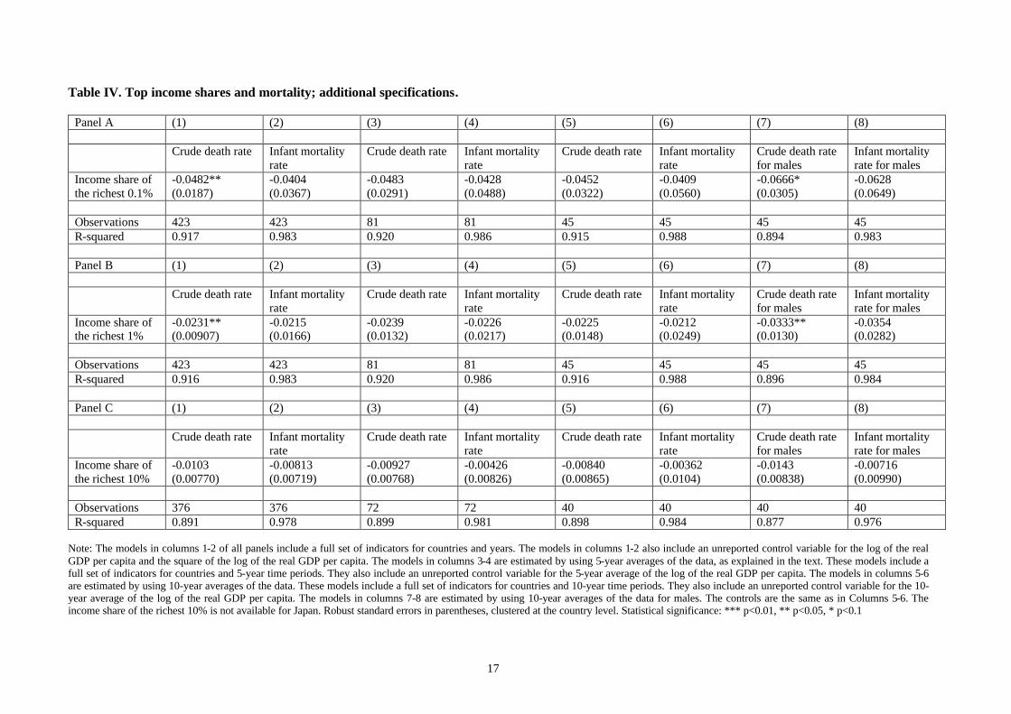
Fourth, we have added the square of GDP per capita to the set of control variables, because there is

earlier evidence according to which the relationship between GDP and mortality is quadratic (Preston,

1975). These specifications reinforce the earlier finding for the existence of a negative relationship

between income inequality and mortality when one uses the income share of the richest 1% (Table IV,

Panel B, Column 1). However, the quantitative magnitude of the estimate remains rather small. The

coefficient of -0.0231 implies that a 10 percentage point increase in the income share of the richest

1% decreases the crude death rate by ~0.2 percentages. In contrast to the results of the baseline

specifications (Table III, Panel A, Column 1), the income share of the richest 0.1% has also a

statistically significant negative effect on the crude death rate (Table IV, Panel A, Column 1).

However, by using the income share of the richest 10% there is no evidence for the statistically

significant relationship (Table IV, Panel C, Column 1). The results for the square of GDP (not

reported) reveal that the negative effect of additional GDP on the crude death rate decreases as GDP

rises. This finding is similar to the one in Leigh and Jencks (2007). Fifth, we have estimated the fixed

effects models, allowing for the first order autocorrelation terms. These models also produce

statistically significant evidence for the negative relationship between the variables of interest (not

reported). However, the statistical significance of these estimates is probably partly driven by the fact

that it is technically not possible to cluster standard errors at the country level at the same time when

one allows for the first order autocorrelation terms to be applied to the models.

13 The data are available at http://iei.uv.es/~rdomenec/human/human.html

10

Table IV here

Sixth, we have estimated the specifications by using 5-year averages of the data for the period 1952-

1998 (the last time period covers the years 1992-1998), because the relationship between income

inequality and mortality may not be instantaneous. Instead, the negative effects of income inequality

on health may take several years to develop (e.g. Gadalla and Fuller-Thomson, 2008). The use of 5-

year averages removes a substantial amount of temporary fluctuations from the variables of interest.

This approach has also been used earlier in the literature on income inequality and economic growth

(e.g. Voitchovsky, 2005). The data that is used to estimate these models consists of 81 observations,

because we have nine countries and nine time periods. These results point out that there is no

statistically significant relationship between top income shares and mortality (Table IV, Panels A-C,

Columns 3-4). The pattern is identical for all three measures of top income shares. Furthermore, we

have estimated specifications by using 10-year averages of the data. (The last time period covers the

years 1992-1998.) The results remain the same (Table IV, Panels A-C, Columns 5-6).

Lastly, we have estimated models for the mortality rates that are calculated separately for males by

using 5-year and 10-year averages of the data, because the baseline estimates (Table III, Panels, A-C,

Column 5) showed that an increase in income inequality seems to be associated with a decrease in the

crude death rate for males. These specifications reveal that the earlier effect prevails by using the

income shares of the richest 0.1% and 1% for both 5- and 10-year averages of the data, but it

disappears by using the income share of the richest 10%. (The results obtained by using 10-year

averages of the data are documented in Columns 7-8 of Table IV.) This pattern is consistent with the

fact that the relationship was statistically weakest in the baseline estimates too when the income share

of the richest 10% was used (Table III, Panel C, Column 5). Also, in accordance with the baseline

estimates, we find that income inequality is not related to infant mortality for males through the use of

10-year averages of the data (Table IV, Panels A-C, Column 8).

5. CONCLUSIONS

The paper uses top income shares measured as the shares of pre-tax income going to the richest 0.1%,

1% and 10% of the population to examine the relationship between income inequality and mortality.

We find that there is no overall relationship between top income shares and mortality in the balanced

panel of nine advanced countries over the period 1952-1998. If anything, the estimates based on

gender breakdown show that there is evidence that an increase in income inequality is associated with

a decrease in the crude death rate for males. This finding is related to earlier research that has found

differences in the effect of income inequality on mortality between genders (e.g. Lochner et al. 2001;

11

Materia et al., 2005). These studies generally find stronger effects of income inequality on mortality

for females.

The most important limitation of the study is arguably the use of the measures of top income shares as

measures of income inequality. Top income shares capture the changes at the top end of the income

distribution and the changes in the Gini coefficient well (Leigh, 2007). However, they do not describe

the changes at the bottom end of the income distribution well. That being said, it is important to note

that, according to Leigh and Jencks (2007:20), almost all of the theoretical arguments for the

existence of a positive relationship between income inequality and mortality should also be valid

when one is measuring income inequality through top income shares.

ACKNOWLEDGEMENTS

I am grateful to Andrew Leigh, Jukka Pirttilä, Ilpo Suoniemi and Hannu Tanninen for very useful

comments and discussions. I am also grateful to Eija Savaja for her help with the data. Paul A.

Dillingham has kindly checked the English language. The usual disclaimer applies.

REFERENCES

Atkinson AB, Brandolini A. 2001. Promise and pitfalls in the use of “secondary” data-sets: Income inequality in OECD countries as a case study. Journal of Economic Literature 39: 771-799.

Atkinson AB, Piketty T. 2007. Top incomes over the Twentieth Century: A Contrast between European and English-Speaking Countries. Oxford: Oxford University Press.

Atkinson AB, Piketty T. 2010. Top incomes: A Global Perspective. Oxford: Oxford University Press.

Babones SJ. 2008. Income inequality and population health: Correlation and causality. Social Science and Medicine 66: 1614-1626.

Böckerman P, Johansson E, Helakorpi S, Uutela A. 2009. Economic inequality and population health: Looking beyond aggregate indicators. Sociology of Health and Illness 31: 422-440.

Cutler D, Lleras-Muney A. 2008. Education and health: Evaluating theories and evidence. In Making Americans Healthier. Social and Economic Policy as Health Policy. Newhouse J, Schoeni G, Kaplan G, Polack H (eds). Russell Sage Press: New York.

de la Fuente A, Doménech R. 2006. Human capital in growth regressions: How much difference does data quality make? Journal of the European Economic Association 4: 1-36.

Deaton A. 2001. Inequalities in income and inequalities in health. In The Causes and Consequences of Increasing Inequality. Welch I (ed.). University of Chicago Press: Chicago.

Deaton A, Lubotsky D. 2003. Mortality, inequality and race in American cities and states. Social Science and Medicine 56: 1139-1153.

12

Eckel C, Grossman P. 2008. Differences in the economic decisions of men and women: Experimental evidence. In Handbook of Experimental Results. Plott C, Smith V (eds). Elsevier: Amsterdam.

Gadalla TM, Fuller-Thomson E. 2008. Examining the lag time between state-level income inequality and individual disabilities: A multilevel analysis. American Journal of Public Health 98: 2187-2190.

Gerdtham UG, Johannesson M. 2004. Absolute income, relative income, income inequality, and mortality. Journal of Human Resources 39: 228-247.

Gravelle H, Sutton M. 2008. Income, relative income, and self-reported health in Britain 1979-2000. Health Economics 18: 125-145.

Gravelle H, Wildman J, Sutton M. 2001. Income, income inequality and health: What can we learn from aggregate data? Social Science and Medicine 54: 577-589.

Hildebrand V, Van Kerm P. 2009. Income inequality and self-rated health status: Evidence from the European Community Household Panel. Demography 46: 805-825.

Judge K, Mulligan J, Benzeval M. 1998. Income inequality and population health. Social Science and Medicine 46: 567-579.

Kravdal Ø. 2008. Does income inequality really influence individual mortality? Results from a ‘fixed-effects analysis’ where constant unobserved municipality characteristics are controlled. Demographic Research 18: 205-232.

Leigh A. 2007. How closely do top income shares track other measures of inequality? Economic Journal 117: F619-F633.

Leigh A, Jencks C. 2007. Inequality and mortality: Long-run evidence from a panel of countries. Journal of Health Economics 26: 1-24.

Leigh A, Jencks C, Smeeding T. 2009. Health and inequality. In The Oxford Handbook of Economic Inequality. Salverda W, Nolan B, Smeeding T (eds). Oxford University Press: Oxford.

Lochner K, Pamuk E, Makuc D, Kennedy BP, Kawachi I. 2001. State-level income inequality and individual mortality risk: A prospective, multilevel study. American Journal of Public Health 91: 385-391.

Lorgelly PK, Lindley J. 2008. What is the relationship between income inequality and health? Evidence from the BHPS. Health Economics 17: 249-265.

Maddison A. 1991. Dynamic Forces in Capitalist Development: A Long-Run Comparative View. Oxford: University Press.

Maddison A. 2003. The World Economy: Historical Statistics. Paris: OECD.

Materia E, Cacciani L, Bugarini G, Cesaroni G, Davoli M, Mirale MP, Vergine L, Baglio G, Simeone G, Perucci CA. 2005. Income inequality and mortality in Italy. The European Journal of Public Health 15: 411-417.

Piketty T, Saez E. 2003. Income inequality in the United States, 1913-1998. Quarterly Journal of Economics 118: 1-39.

Preston SH. 1975. The changing relation between mortality and level of economic development. Population Studies 29: 231-248.

Roine J, Waldenström D, Vlachos J. 2009. The long-run determinants of inequality: What can we learn from top income data? Journal of Public Economics 93: 974-988.

Saez E. 2005. Top incomes in the United States and Canada over the twentieth century. Journal of the European Economic Association 3: 402-411.

Subramanian SV, Kawachi I. 2004. Income inequality and health: What have we learned so far? Epidemiologic Review 26: 78-91.

13

Voitchovsky S. 2005. Does the profile in income inequality matter for economic growth? Journal of Economic Growth 10: 273-296.

Wagstaff A, van Doorslaer E. 2000. Income inequality and health: What does the literature tell us? Annual Review of Public Health 21: 543-567.

Waldmann RJ. 1992. Income distribution and infant mortality. Quarterly Journal of Economics 107: 1283-1302.

Wilkinson RG. 1996. Unhealthy Societies: The Afflictions of Inequality. London: Routledge.

Wilkinson RG. Pickett KE. 2006. Income inequality and population health: A review and explanation of the evidence. Social Science and Medicine 62: 1768-1784.

Wilkinson RG. Pickett KE. 2009. The Spirit Level. Why More Equal Societies Almost Always Do Better. London: Penguin Books Ltd.

14

Table I. Descriptive statistics of the variables. N Mean St. Dev. Dependent variables Log of the crude death rate 423 2.1751 0.1781 Log of the infant mortality rate 423 2.5240 0.5720 Log of the crude death rate for females 423 2.0862 0.2020 Log of the infant mortality rate for females 423 2.3914 0.5690 Log of the crude death rate for males 423 2.2567 0.1645 Log of the infant mortality rate for males 423 2.6348 0.5754 Explanatory variables Income share of the richest 0.1% 423 2.0093 0.8447 Income share of the richest 1% 423 7.7863 1.9155 Income share of the richest 10% 376 31.4975 4.1976 Log of the real GDP per capita ($ 1000s) 423 9.4194 0.3934

Note: The income share of the richest 10% is not available for Japan.

15

Table II. Top income shares and mortality; the importance of fixed country effects.

Panel A (1) (2) (3) (4) Crude death rate Crude death rate Infant mortality

rate Infant mortality rate

Income share of the richest 0.1%

-0.0153 (0.0340)

-0.0280 (0.0176)

0.0899 (0.0533)

-0.0922** (0.0290)

Fixed country effects

No Yes No Yes

Fixed year effects No No No No Observations 423 423 423 423 R-squared 0.016 0.893 0.688 0.935 Panel B (1) (2) (3) (4) Crude death rate Crude death rate Infant mortality


Income share of the richest 1%

-0.00779 (0.0179)

-0.0132 (0.00798)

0.0505* (0.0261)

-0.0343** (0.0108)


No Yes No Yes

Fixed year effects No No No No Observations 423 423 423 423 R-squared 0.018 0.893 0.698 0.931 Panel C (1) (2) (3) (4) Crude death rate Crude death rate Infant mortality



-0.00883 (0.00983)

-0.00759 (0.00452)

0.0246* (0.0127)

-0.0163* (0.00701)


No Yes No Yes

Fixed year effects No No No No Observations 376 376 376 376 R-squared 0.109 0.878 0.726 0.933

Note: The models include a full set of indicators for countries and years, as indicated. All 12 models include an unreported control variable for the log of the real GDP per capita. The income share of the richest 10% is not available for Japan. Robust standard errors in parentheses, clustered at the country level. Statistical significance: *** p<0.01, ** p<0.05, * p<0.1

16

Table III. Top income shares and mortality; baseline specifications.

Panel A (1) (2) (3) (4) (5) (6) Crude death


Crude death rate for females

Infant mortality rate for females

Crude death rate for males

Infant mortality rate for males


-0.0436 (0.0256)

-0.0366 (0.0439)

-0.0280 (0.0326)

-0.0355 (0.0440)

-0.0568** (0.0202)

-0.0375 (0.0440)

Observations 423 423 423 423 423 423 R-squared 0.906 0.982 0.915 0.980 0.889 0.981 Panel B (1) (2) (3) (4) (5) (6) Crude death







-0.0222* (0.0117)

-0.0207 (0.0196)

-0.0155 (0.0153)

-0.0201 (0.0197)

-0.0280** (0.00892)

-0.0211 (0.0197)

Observations 423 423 423 423 423 423 R-squared 0.907 0.982 0.916 0.980 0.890 0.982 Panel C (1) (2) (3) (4) (5) (6) Crude death







-0.00870 (0.00668)

-0.00455 (0.00756)

-0.00496 (0.00731)

-0.00494 (0.00766)

-0.0122* (0.00626)

-0.00425 (0.00759)

Observations 376 376 376 376 376 376 R-squared 0.888 0.977 0.898 0.975 0.876 0.976

Note: All 18 models include a full set of indicators for countries and years. All models of all panels also include an unreported control variable for the log of the real GDP per capita. The income share of the richest 10% is not available for Japan. Robust standard errors in parentheses, clustered at the country level. Statistical significance: *** p<0.01, ** p<0.05, * p<0.1

17

Table IV. Top income shares and mortality; additional specifications.

Panel A (1) (2) (3) (4) (5) (6) (7) (8) Crude death rate Infant mortality

rate Crude death rate Infant mortality


rate Crude death rate for males



-0.0482** (0.0187)

-0.0404 (0.0367)

-0.0483 (0.0291)

-0.0428 (0.0488)

-0.0452 (0.0322)

-0.0409 (0.0560)

-0.0666* (0.0305)

-0.0628 (0.0649)

Observations 423 423 81 81 45 45 45 45 R-squared 0.917 0.983 0.920 0.986 0.915 0.988 0.894 0.983 Panel B (1) (2) (3) (4) (5) (6) (7) (8) Crude death rate Infant mortality






-0.0231** (0.00907)

-0.0215 (0.0166)

-0.0239 (0.0132)

-0.0226 (0.0217)

-0.0225 (0.0148)

-0.0212 (0.0249)

-0.0333** (0.0130)

-0.0354 (0.0282)

Observations 423 423 81 81 45 45 45 45 R-squared 0.916 0.983 0.920 0.986 0.916 0.988 0.896 0.984 Panel C (1) (2) (3) (4) (5) (6) (7) (8) Crude death rate Infant mortality






-0.0103 (0.00770)

-0.00813 (0.00719)

-0.00927 (0.00768)

-0.00426 (0.00826)

-0.00840 (0.00865)

-0.00362 (0.0104)

-0.0143 (0.00838)

-0.00716 (0.00990)

Observations 376 376 72 72 40 40 40 40 R-squared 0.891 0.978 0.899 0.981 0.898 0.984 0.877 0.976

Note: The models in columns 1-2 of all panels include a full set of indicators for countries and years. The models in columns 1-2 also include an unreported control variable for the log of the real GDP per capita and the square of the log of the real GDP per capita. The models in columns 3-4 are estimated by using 5-year averages of the data, as explained in the text. These models include a full set of indicators for countries and 5-year time periods. They also include an unreported control variable for the 5-year average of the log of the real GDP per capita. The models in columns 5-6 are estimated by using 10-year averages of the data. These models include a full set of indicators for countries and 10-year time periods. They also include an unreported control variable for the 10-year average of the log of the real GDP per capita. The models in columns 7-8 are estimated by using 10-year averages of the data for males. The controls are the same as in Columns 5-6. The income share of the richest 10% is not available for Japan. Robust standard errors in parentheses, clustered at the country level. Statistical significance: *** p<0.01, ** p<0.05, * p<0.1

Government & Nonprofit

Top income shares and mortality: Evidence from advanced countries