Embed Size (px)
Citation preview
Finite ElementAnalysis
Sujith Jose
Introduction
Steps in FiniteElementAnalysis
Finite ElementDiscretization
ElementaryGoverningEquations
Assembling of allelements
Solving theresultingequations
i.IterationMethod
ii.Band MatrixMethod
Example
References
Finite Element Analysis - The Basics
Sujith Jose
University of California, Los Angeles
May 31, 2016
Finite ElementAnalysis
Sujith Jose
Introduction
Steps in FiniteElementAnalysis
Finite ElementDiscretization
ElementaryGoverningEquations
Assembling of allelements
Solving theresultingequations
i.IterationMethod
ii.Band MatrixMethod
Example
References
Overview
1 Introduction
2 Steps in Finite Element AnalysisFinite Element DiscretizationElementary Governing EquationsAssembling of all elementsSolving the resulting equations
i.Iteration Methodii.Band Matrix Method
3 Example
4 References
Finite ElementAnalysis
Sujith Jose
Introduction
Steps in FiniteElementAnalysis
Finite ElementDiscretization
ElementaryGoverningEquations
Assembling of allelements
Solving theresultingequations
i.IterationMethod
ii.Band MatrixMethod
Example
References
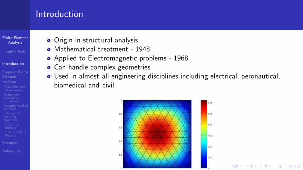
Introduction
Origin in structural analysisMathematical treatment - 1948Applied to Electromagnetic problems - 1968Can handle complex geometriesUsed in almost all engineering disciplines including electrical, aeronautical,biomedical and civil

Finite ElementAnalysis
Sujith Jose
Introduction
Steps in FiniteElementAnalysis
Finite ElementDiscretization
ElementaryGoverningEquations
Assembling of allelements
Solving theresultingequations
i.IterationMethod
ii.Band MatrixMethod
Example
References
Steps in Finite Element Analysis
1 Discretize the solution region into elements
2 Derive governing equations for one element
3 Assemble all elements
4 Solving system of equations obtained
Finite ElementAnalysis
Sujith Jose
Introduction
Steps in FiniteElementAnalysis
Finite ElementDiscretization
ElementaryGoverningEquations
Assembling of allelements
Solving theresultingequations
i.IterationMethod
ii.Band MatrixMethod
Example
References
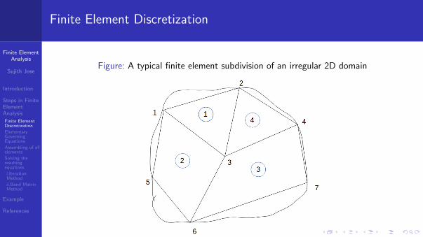
Finite Element Discretization
Figure: A typical finite element subdivision of an irregular 2D domain
Finite ElementAnalysis
Sujith Jose
Introduction
Steps in FiniteElementAnalysis
Finite ElementDiscretization
ElementaryGoverningEquations
Assembling of allelements
Solving theresultingequations
i.IterationMethod
ii.Band MatrixMethod
Example
References
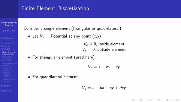
Finite Element Discretization
Consider a single element (triangular or quadrilateral)
Let Ve = Potential at any point (x,y)
Ve 6= 0, inside elementVe = 0, outside element
For triangular element (used here)
Ve = a + bx + cy
For quadrilateral element
Ve = a + bx + cy + dxy

Finite ElementAnalysis
Sujith Jose
Introduction
Steps in FiniteElementAnalysis
Finite ElementDiscretization
ElementaryGoverningEquations
Assembling of allelements
Solving theresultingequations
i.IterationMethod
ii.Band MatrixMethod
Example
References
Finite Element Discretization
Consider triangular element,
Ve(x , y) = a + bx + cy
Linear variation of potential is the same as assuming that electric field is uniformwithin the element.i.e
~Ee = −∇Ve = −(b ~ax + c ~ay )
Finite ElementAnalysis
Sujith Jose
Introduction
Steps in FiniteElementAnalysis
Finite ElementDiscretization
ElementaryGoverningEquations
Assembling of allelements
Solving theresultingequations
i.IterationMethod
ii.Band MatrixMethod
Example
References
Elementary Governing Equations
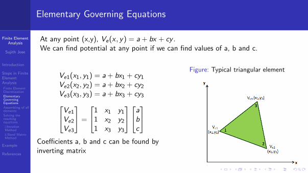
At any point (x,y), Ve(x , y) = a + bx + cy .We can find potential at any point if we can find values of a, b and c.
Ve1(x1, y1) = a + bx1 + cy1Ve2(x2, y2) = a + bx2 + cy2Ve3(x3, y3) = a + bx3 + cy3Ve1
Ve2
Ve3
=
1 x1 y11 x2 y21 x3 y3
abc
Coefficients a, b and c can be found byinverting matrix
Figure: Typical triangular element
Finite ElementAnalysis
Sujith Jose
Introduction
Steps in FiniteElementAnalysis
Finite ElementDiscretization
ElementaryGoverningEquations
Assembling of allelements
Solving theresultingequations
i.IterationMethod
ii.Band MatrixMethod
Example
References
Elementary Governing Equations
abc
=
1 x1 y11 x2 y21 x3 y3
−1 Ve1
Ve2
Ve3
abc
= 1DET
(x2y3 − x3y2) (x3y1 − x1y3) (x1y2 − x2y1)(y2 − y3) (y3 − y1) (y1 − y2)(x3 − x2) (x1 − x3) (x2 − x1)
Ve1
Ve2
Ve3
Let
DET =
∣∣∣∣∣∣1 x1 y11 x2 y21 x3 y3
∣∣∣∣∣∣ = 2A
Finite ElementAnalysis
Sujith Jose
Introduction
Steps in FiniteElementAnalysis
Finite ElementDiscretization
ElementaryGoverningEquations
Assembling of allelements
Solving theresultingequations
i.IterationMethod
ii.Band MatrixMethod
Example
References
Elementary Governing Equations
abc
= 12A
(x2y3 − x3y2) (x3y1 − x1y3) (x1y2 − x2y1)(y2 − y3) (y3 − y1) (y1 − y2)(x3 − x2) (x1 − x3) (x2 − x1)
Ve1
Ve2
Ve3
Ve(x , y) = a + bx + cy =
[1 x y
] abc
Ve(x , y) =[1 x y
]12A
(x2y3 − x3y2) (x3y1 − x1y3) (x1y2 − x2y1)(y2 − y3) (y3 − y1) (y1 − y2)(x3 − x2) (x1 − x3) (x2 − x1)
Ve1
Ve2
Ve3
Ve(x , y) = 12A
[α1 α2 α3
] Ve1
Ve2
Ve3
=3∑
i=1αi (x , y)Vei
Finite ElementAnalysis
Sujith Jose
Introduction
Steps in FiniteElementAnalysis
Finite ElementDiscretization
ElementaryGoverningEquations
Assembling of allelements
Solving theresultingequations
i.IterationMethod
ii.Band MatrixMethod
Example
References
Elementary Governing Equations
Potential Ve(x , y) at any point (x,y) within the element (provided the potential atvertices)
Ve(x , y) =3∑
i=1
αi (x , y)Vei
where
α1 =1
2A[(x2y3 − x3y2) + (y2 − y3)x + (x3 − x2)y ] (1)
α2 =1
2A[(x3y1 − x1y3) + (y3 − y1)x + (x1 − x3)y ] (2)
α3 =1
2A[(x1y2 − x2y1) + (y1 − y2)x + (x2 − x1)y ] (3)
αi are called linear interpolation functions or element shape functions
Finite ElementAnalysis
Sujith Jose
Introduction
Steps in FiniteElementAnalysis
Finite ElementDiscretization
ElementaryGoverningEquations
Assembling of allelements
Solving theresultingequations
i.IterationMethod
ii.Band MatrixMethod
Example
References
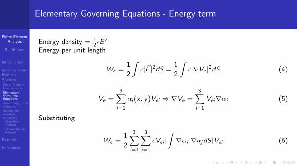
Elementary Governing Equations - Energy term
Energy density = 12εE
2
Energy per unit length
We =1
2
∫ε|~E |2dS =
1
2
∫ε|∇Ve |2dS (4)
Ve =3∑
i=1
αi (x , y)Vei ⇒ ∇Ve =3∑
i=1
Vei∇αi (5)
Substituting
We =1
2
3∑i=1
3∑j=1
εVei |∫∇αi .∇αjdS |Vei (6)
Finite ElementAnalysis
Sujith Jose
Introduction
Steps in FiniteElementAnalysis
Finite ElementDiscretization
ElementaryGoverningEquations
Assembling of allelements
Solving theresultingequations
i.IterationMethod
ii.Band MatrixMethod
Example
References
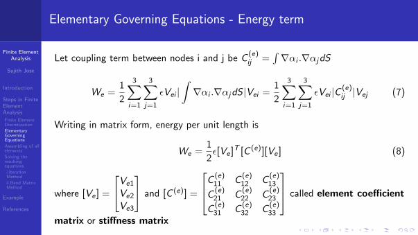
Elementary Governing Equations - Energy term
Let coupling term between nodes i and j be C(e)ij =
∫∇αi .∇αjdS
We =1
2
3∑i=1
3∑j=1
εVei |∫∇αi .∇αjdS |Vei =
1
2
3∑i=1
3∑j=1
εVei |C(e)ij |Vej (7)
Writing in matrix form, energy per unit length is
We =1
2ε[Ve ]T [C (e)][Ve ] (8)
where [Ve ] =
Ve1
Ve2
Ve3
and [C (e)] =
C(e)11 C
(e)12 C
(e)13
C(e)21 C
(e)22 C
(e)23
C(e)31 C
(e)32 C
(e)33
called element coefficient
matrix or stiffness matrix
Finite ElementAnalysis
Sujith Jose
Introduction
Steps in FiniteElementAnalysis
Finite ElementDiscretization
ElementaryGoverningEquations
Assembling of allelements
Solving theresultingequations
i.IterationMethod
ii.Band MatrixMethod
Example
References
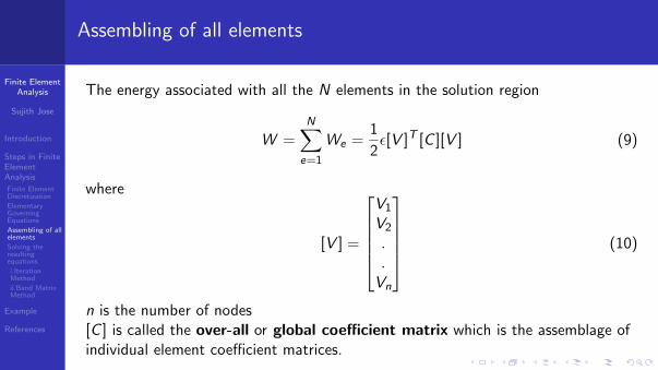
Assembling of all elements
The energy associated with all the N elements in the solution region
W =N∑
e=1
We =1
2ε[V ]T [C ][V ] (9)
where
[V ] =
V1
V2
.
.Vn
(10)
n is the number of nodes[C ] is called the over-all or global coefficient matrix which is the assemblage ofindividual element coefficient matrices.
Finite ElementAnalysis
Sujith Jose
Introduction
Steps in FiniteElementAnalysis
Finite ElementDiscretization
ElementaryGoverningEquations
Assembling of allelements
Solving theresultingequations
i.IterationMethod
ii.Band MatrixMethod
Example
References
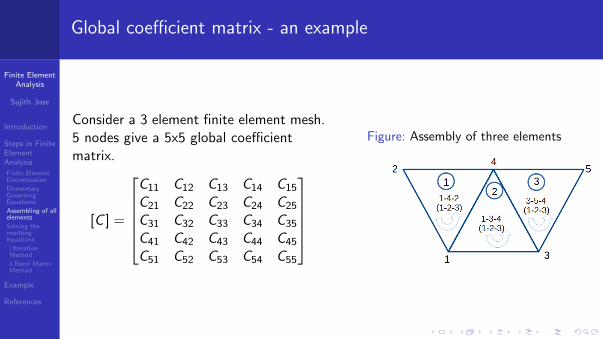
Global coefficient matrix - an example
Consider a 3 element finite element mesh.5 nodes give a 5x5 global coefficientmatrix.
[C ] =
C11 C12 C13 C14 C15
C21 C22 C23 C24 C25
C31 C32 C33 C34 C35
C41 C42 C43 C44 C45
C51 C52 C53 C54 C55
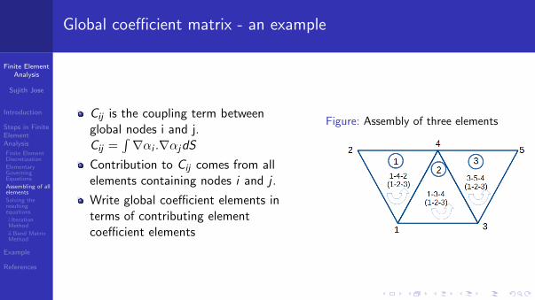
Figure: Assembly of three elements
Finite ElementAnalysis
Sujith Jose
Introduction
Steps in FiniteElementAnalysis
Finite ElementDiscretization
ElementaryGoverningEquations
Assembling of allelements
Solving theresultingequations
i.IterationMethod
ii.Band MatrixMethod
Example
References
Global coefficient matrix - an example
Cij is the coupling term betweenglobal nodes i and j.Cij =
∫∇αi .∇αjdS
Contribution to Cij comes from allelements containing nodes i and j .
Write global coefficient elements interms of contributing elementcoefficient elements
Figure: Assembly of three elements
Finite ElementAnalysis
Sujith Jose
Introduction
Steps in FiniteElementAnalysis
Finite ElementDiscretization
ElementaryGoverningEquations
Assembling of allelements
Solving theresultingequations
i.IterationMethod
ii.Band MatrixMethod
Example
References
Global coefficient matrix - an example
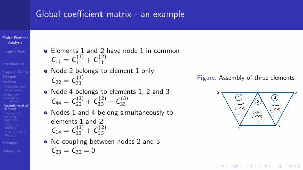
Elements 1 and 2 have node 1 in commonC11 = C
(1)11 + C
(2)11
Node 2 belongs to element 1 only
C22 = C(1)33
Node 4 belongs to elements 1, 2 and 3
C44 = C(1)22 + C
(2)33 + C
(3)33
Nodes 1 and 4 belong simultaneously toelements 1 and 2C14 = C
(1)12 + C
(2)13
No coupling between nodes 2 and 3C23 = C32 = 0
Figure: Assembly of three elements
Finite ElementAnalysis
Sujith Jose
Introduction
Steps in FiniteElementAnalysis
Finite ElementDiscretization
ElementaryGoverningEquations
Assembling of allelements
Solving theresultingequations
i.IterationMethod
ii.Band MatrixMethod
Example
References
Global coefficient matrix - an example
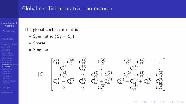
The global coefficient matrix
Symmetric (Cij = Cji )
Sparse
Singular
[C ] =
C
(1)11 + C
(2)11 C
(1)13 C
(2)12 C
(1)12 + C
(2)13 0
C(1)31 C
(1)33 0 C
(1)32 0
C(2)21 0 C
(2)22 + C
(3)11 C
(2)23 + C
(3)13 C
(3)13
C(1)21 + C
(2)31 C
(1)23 C
(2)32 + C
(3)31 C
(1)22 + C
(2)33 + C
(3)33 C
(3)32
0 0 C(3)21 C
(3)23 C
(3)22
Finite ElementAnalysis
Sujith Jose
Introduction
Steps in FiniteElementAnalysis
Finite ElementDiscretization
ElementaryGoverningEquations
Assembling of allelements
Solving theresultingequations
i.IterationMethod
ii.Band MatrixMethod
Example
References
Global coefficient matrix - an example
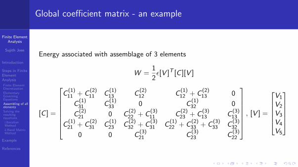
Energy associated with assemblage of 3 elements
W =1
2ε[V ]T [C ][V ]
[C ] =
C
(1)11 + C
(2)11 C
(1)13 C
(2)12 C
(1)12 + C
(2)13 0
C(1)31 C
(1)33 0 C
(1)32 0
C(2)21 0 C
(2)22 + C
(3)11 C
(2)23 + C
(3)13 C
(3)13
C(1)21 + C
(2)31 C
(1)23 C
(2)32 + C
(3)31 C
(1)22 + C
(2)33 + C
(3)33 C
(3)32
0 0 C(3)21 C
(3)23 C
(3)22
, [V ] =
V1
V2
V3
V4
V5

Finite ElementAnalysis
Sujith Jose
Introduction
Steps in FiniteElementAnalysis
Finite ElementDiscretization
ElementaryGoverningEquations
Assembling of allelements
Solving theresultingequations
i.IterationMethod
ii.Band MatrixMethod
Example
References
Solving the resulting equations
Laplace’s (or Poisson’s ) equation is satisfied when the total energy in thesolution region is minimum
Hence, ∂W∂V1
= ∂W∂V2
= ... = ∂W∂Vn
= 0
Finite ElementAnalysis
Sujith Jose
Introduction
Steps in FiniteElementAnalysis
Finite ElementDiscretization
ElementaryGoverningEquations
Assembling of allelements
Solving theresultingequations
i.IterationMethod
ii.Band MatrixMethod
Example
References
Solving the resulting equations
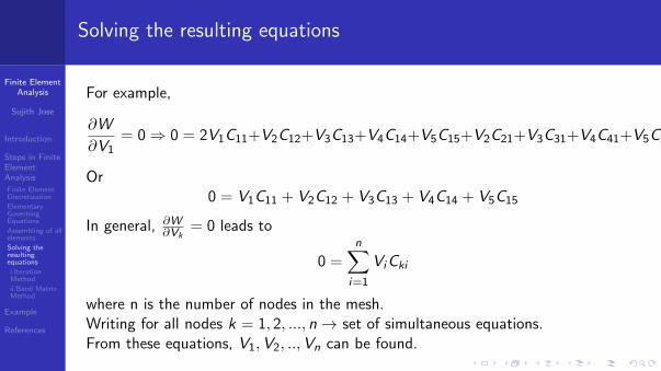
For example,
∂W
∂V1= 0⇒ 0 = 2V1C11+V2C12+V3C13+V4C14+V5C15+V2C21+V3C31+V4C41+V5C51
Or0 = V1C11 + V2C12 + V3C13 + V4C14 + V5C15
In general, ∂W∂Vk
= 0 leads to
0 =n∑
i=1
ViCki
where n is the number of nodes in the mesh.Writing for all nodes k = 1, 2, ..., n→ set of simultaneous equations.From these equations, V1,V2, ..,Vn can be found.
Finite ElementAnalysis
Sujith Jose
Introduction
Steps in FiniteElementAnalysis
Finite ElementDiscretization
ElementaryGoverningEquations
Assembling of allelements
Solving theresultingequations
i.IterationMethod
ii.Band MatrixMethod
Example
References
Solving the resulting equationsIteration method
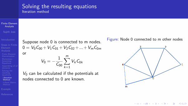
Suppose node 0 is connected to m nodes.0 = V0C00 +V1C01 +V2C02 + ...+VmC0m
or
V0 = − 1
C00
m∑k=1
VkC0k
V0 can be calculated if the potentials atnodes connected to 0 are known.
Figure: Node 0 connected to m other nodes
Finite ElementAnalysis
Sujith Jose
Introduction
Steps in FiniteElementAnalysis
Finite ElementDiscretization
ElementaryGoverningEquations
Assembling of allelements
Solving theresultingequations
i.IterationMethod
ii.Band MatrixMethod
Example
References
Solving the resulting equationsIteration method
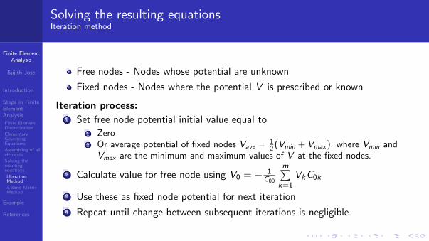
Free nodes - Nodes whose potential are unknown
Fixed nodes - Nodes where the potential V is prescribed or known
Iteration process:1 Set free node potential initial value equal to
1 Zero2 Or average potential of fixed nodes Vave = 1
2 (Vmin + Vmax ), where Vmin andVmax are the minimum and maximum values of V at the fixed nodes.
2 Calculate value for free node using V0 = − 1C00
m∑k=1
VkC0k
3 Use these as fixed node potential for next iteration
4 Repeat until change between subsequent iterations is negligible.
Finite ElementAnalysis
Sujith Jose
Introduction
Steps in FiniteElementAnalysis
Finite ElementDiscretization
ElementaryGoverningEquations
Assembling of allelements
Solving theresultingequations
i.IterationMethod
ii.Band MatrixMethod
Example
References
Solving the resulting equationsBand Matrix Method
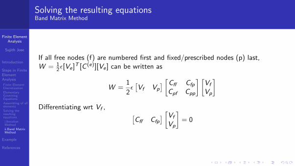
If all free nodes (f) are numbered first and fixed/prescribed nodes (p) last,W = 1
2ε[Ve ]T [C (e)][Ve ] can be written as
W =1
2ε[Vf Vp
] [Cff Cfp
Cpf Cpp
] [Vf
Vp
]Differentiating wrt Vf , [
Cff Cfp
] [Vf
Vp
]= 0
Finite ElementAnalysis
Sujith Jose
Introduction
Steps in FiniteElementAnalysis
Finite ElementDiscretization
ElementaryGoverningEquations
Assembling of allelements
Solving theresultingequations
i.IterationMethod
ii.Band MatrixMethod
Example
References
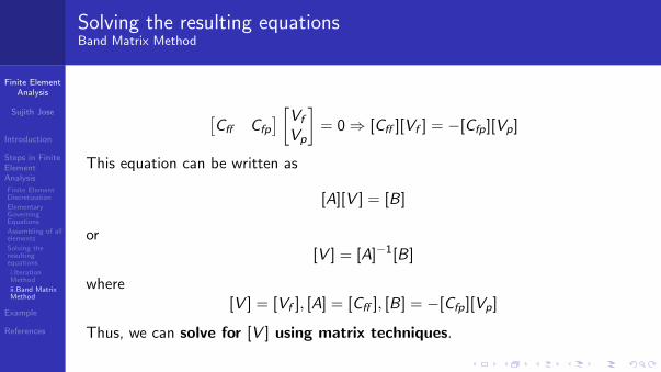
Solving the resulting equationsBand Matrix Method
[Cff Cfp
] [Vf
Vp
]= 0⇒ [Cff ][Vf ] = −[Cfp][Vp]
This equation can be written as
[A][V ] = [B]
or[V ] = [A]−1[B]
where[V ] = [Vf ], [A] = [Cff ], [B] = −[Cfp][Vp]
Thus, we can solve for [V ] using matrix techniques.
Finite ElementAnalysis
Sujith Jose
Introduction
Steps in FiniteElementAnalysis
Finite ElementDiscretization
ElementaryGoverningEquations
Assembling of allelements
Solving theresultingequations
i.IterationMethod
ii.Band MatrixMethod
Example
References
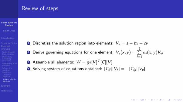
Review of steps
1 Discretize the solution region into elements: Ve = a + bx + cy
2 Derive governing equations for one element: Ve(x , y) =3∑
i=1αi (x , y)Vei
3 Assemble all elements: W = 12ε[V ]T [C ][V ]
4 Solving system of equations obtained: [Cff ][Vf ] = −[Cfp][Vp]
Finite ElementAnalysis
Sujith Jose
Introduction
Steps in FiniteElementAnalysis
Finite ElementDiscretization
ElementaryGoverningEquations
Assembling of allelements
Solving theresultingequations
i.IterationMethod
ii.Band MatrixMethod
Example
References
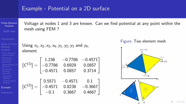
Example - Potential on a 2D surface
Voltage at nodes 1 and 3 are known. Can we find potential at any point within themesh using FEM ?
Using x1, x2, x3, x4, y1, y2, y3 and y4,element
[C (1)] =
1.236 −0.7786 −0.4571−0.7786 0.6929 0.0857−0.4571 0.0857 0.3714
[C (2)] =
0.5571 −0.4571 0.1−0.4571 0.8238 −0.3667−0.1 0.3667 0.4667
Figure: Two element mesh
Finite ElementAnalysis
Sujith Jose
Introduction
Steps in FiniteElementAnalysis
Finite ElementDiscretization
ElementaryGoverningEquations
Assembling of allelements
Solving theresultingequations
i.IterationMethod
ii.Band MatrixMethod
Example
References
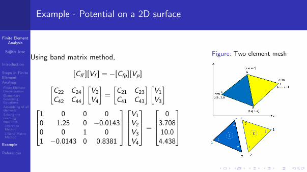
Example - Potential on a 2D surface
Using band matrix method,
[Cff ][Vf ] = −[Cfp][Vp][C22 C24
C42 C44
] [V2
V4
]=
[C21 C23
C41 C43
] [V1
V3
]
1 0 0 00 1.25 0 −0.01430 0 1 01 −0.0143 0 0.8381
V1
V2
V3
V4
=
0
3.70810.0
4.438
Figure: Two element mesh
Finite ElementAnalysis
Sujith Jose
Introduction
Steps in FiniteElementAnalysis
Finite ElementDiscretization
ElementaryGoverningEquations
Assembling of allelements
Solving theresultingequations
i.IterationMethod
ii.Band MatrixMethod
Example
References
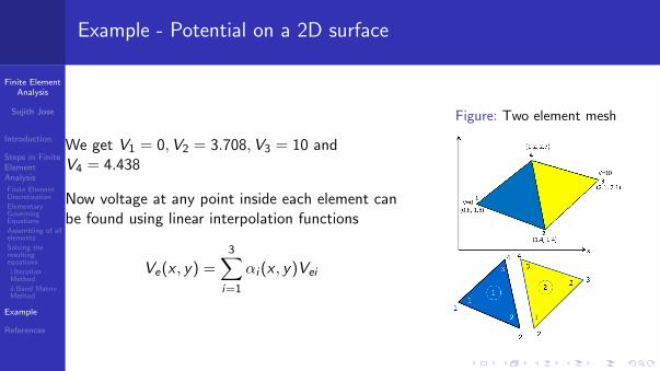
Example - Potential on a 2D surface
We get V1 = 0,V2 = 3.708,V3 = 10 andV4 = 4.438
Now voltage at any point inside each element canbe found using linear interpolation functions
Ve(x , y) =3∑
i=1
αi (x , y)Vei
Figure: Two element mesh
Finite ElementAnalysis
Sujith Jose
Introduction
Steps in FiniteElementAnalysis
Finite ElementDiscretization
ElementaryGoverningEquations
Assembling of allelements
Solving theresultingequations
i.IterationMethod
ii.Band MatrixMethod
Example
References
References
Matthew Sadiku (1989)
A Simple Introduction to Finite Element Analysis of Electromagnetic Problems
IEEE Transactions on Education 32(2), 85 - 93.
Jianming Jin (2002)
The Finite Element Method in Electromagnetics
Second Edition

Finite ElementAnalysis
Sujith Jose
Introduction
Steps in FiniteElementAnalysis
Finite ElementDiscretization
ElementaryGoverningEquations
Assembling of allelements
Solving theresultingequations
i.IterationMethod
ii.Band MatrixMethod
Example
References
Questions?
Finite ElementAnalysis
Sujith Jose
Introduction
Steps in FiniteElementAnalysis
Finite ElementDiscretization
ElementaryGoverningEquations
Assembling of allelements
Solving theresultingequations
i.IterationMethod
ii.Band MatrixMethod
Example
References
Appendix - Boundary value problems
A boundary value problem can be defined by a governing differential equation in adomain Ω:
Lφ = f
together with boundary conditions on the boundary that encloses the domain.Approximate solutions to boundary value problems can be found using Ritz orGalerkin’s method.
Finite ElementAnalysis
Sujith Jose
Introduction
Steps in FiniteElementAnalysis
Finite ElementDiscretization
ElementaryGoverningEquations
Assembling of allelements
Solving theresultingequations
i.IterationMethod
ii.Band MatrixMethod
Example
References
Appendix - Ritz method
Boundary value problem is formulated in terms of a variational expressioncalled functional.
Minimum of this functional corresponds to the governing differential equationunder the given boundary conditions.
Approximate solution is then obtained by minimizing the functional withrespect to variables that define a certain approximation to the solution.
Finite ElementAnalysis
Sujith Jose
Introduction
Steps in FiniteElementAnalysis
Finite ElementDiscretization
ElementaryGoverningEquations
Assembling of allelements
Solving theresultingequations
i.IterationMethod
ii.Band MatrixMethod
Example
References
Appendix - Galerkin’s method
This method is one of the weighted residual methods i.e. seek the solution byweighting the residual of the differential equation.
Assume that φ is an approximate solution to boundary value problem. Then,nonzero residual
r = Lφ− f 6= 0
The best approximation for φ will be the one that reduces residual r to leastvalue at all points of Ω.
Ri =
∫wi rdΩ = 0
where Ri denote weighted residual integrals and wi are chosen weightingfunctions.