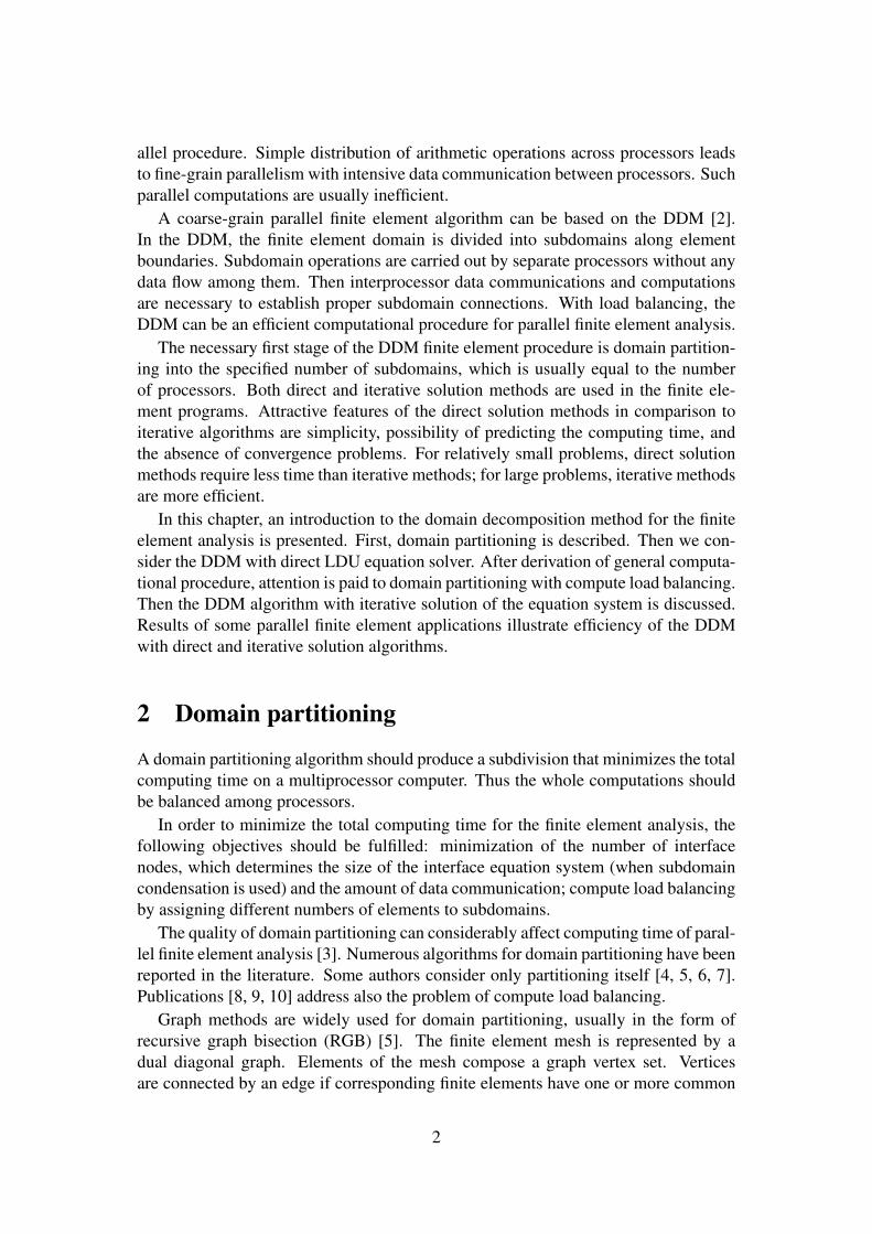
Mesh Partitioning Techniques and DomainDecomposition Methods (Ed. F.Magoules)

Saxe-Coburg, Stirling, Scotland, 2007, pp. 119-142.

Basics of the Domain DecompositionMethod for Finite Element Analysis

G.P.NikishkovUniversity of Aizu, Aizu-Wakamatsu City, Fukushima, Japan

Abstract

An introduction to the domain decomposition method for parallel finite element anal-ysis is presented. The domain decomposition method allows decomposition of large-size problem solutions to solutions of several smaller size problems. Algorithms ofdomain partitioning with compute load balancing as well as direct and iterative solu-tion techniques are considered.

Keywords: Finite element method, domain decomposition, partitioning, parallel.

1 Introduction

Various appications of the domain decomposition method (DDM) have a long his-tory in computational science. The DDM in the form of substructuring was used infinite element analysis soon after introduction of the finite element method in engi-neering practice [1]. The reason for employing the substructuring technique was thesmall memory of computers. To solve large-scale problems, a structure (domain) wasdivided into substructures (subdomains) that fit into computer memory.

Computer memory grows but demand for solution of large-scale problems is al-ways ahead of computer capabilities. Large-scale scientific and engineering simu-lations performed with the finite element method often require very long computingtime. While limited progress can be made with improvement of numerical algorithms,the radical time reduction can be reached with multiprocessor computations. In or-der to perform finite element analysis on a parallel computer, computation should bedistributed across processors.

Element-wise operations, such as calculation of element matrices, are easy to par-allelize. More difficult is to transform solution of a global equation system into a par-

1

allel procedure. Simple distribution of arithmetic operations across processors leadsto fine-grain parallelism with intensive data communication between processors. Suchparallel computations are usually inefficient.

A coarse-grain parallel finite element algorithm can be based on the DDM [2].In the DDM, the finite element domain is divided into subdomains along elementboundaries. Subdomain operations are carried out by separate processors without anydata flow among them. Then interprocessor data communications and computationsare necessary to establish proper subdomain connections. With load balancing, theDDM can be an efficient computational procedure for parallel finite element analysis.

The necessary first stage of the DDM finite element procedure is domain partition-ing into the specified number of subdomains, which is usually equal to the numberof processors. Both direct and iterative solution methods are used in the finite ele-ment programs. Attractive features of the direct solution methods in comparison toiterative algorithms are simplicity, possibility of predicting the computing time, andthe absence of convergence problems. For relatively small problems, direct solutionmethods require less time than iterative methods; for large problems, iterative methodsare more efficient.

In this chapter, an introduction to the domain decomposition method for the finiteelement analysis is presented. First, domain partitioning is described. Then we con-sider the DDM with direct LDU equation solver. After derivation of general computa-tional procedure, attention is paid to domain partitioning with compute load balancing.Then the DDM algorithm with iterative solution of the equation system is discussed.Results of some parallel finite element applications illustrate efficiency of the DDMwith direct and iterative solution algorithms.

2 Domain partitioning

A domain partitioning algorithm should produce a subdivision that minimizes the totalcomputing time on a multiprocessor computer. Thus the whole computations shouldbe balanced among processors.

In order to minimize the total computing time for the finite element analysis, thefollowing objectives should be fulfilled: minimization of the number of interfacenodes, which determines the size of the interface equation system (when subdomaincondensation is used) and the amount of data communication; compute load balancingby assigning different numbers of elements to subdomains.

The quality of domain partitioning can considerably affect computing time of paral-lel finite element analysis [3]. Numerous algorithms for domain partitioning have beenreported in the literature. Some authors consider only partitioning itself [4, 5, 6, 7].Publications [8, 9, 10] address also the problem of compute load balancing.

Graph methods are widely used for domain partitioning, usually in the form ofrecursive graph bisection (RGB) [5]. The finite element mesh is represented by adual diagonal graph. Elements of the mesh compose a graph vertex set. Verticesare connected by an edge if corresponding finite elements have one or more common

2

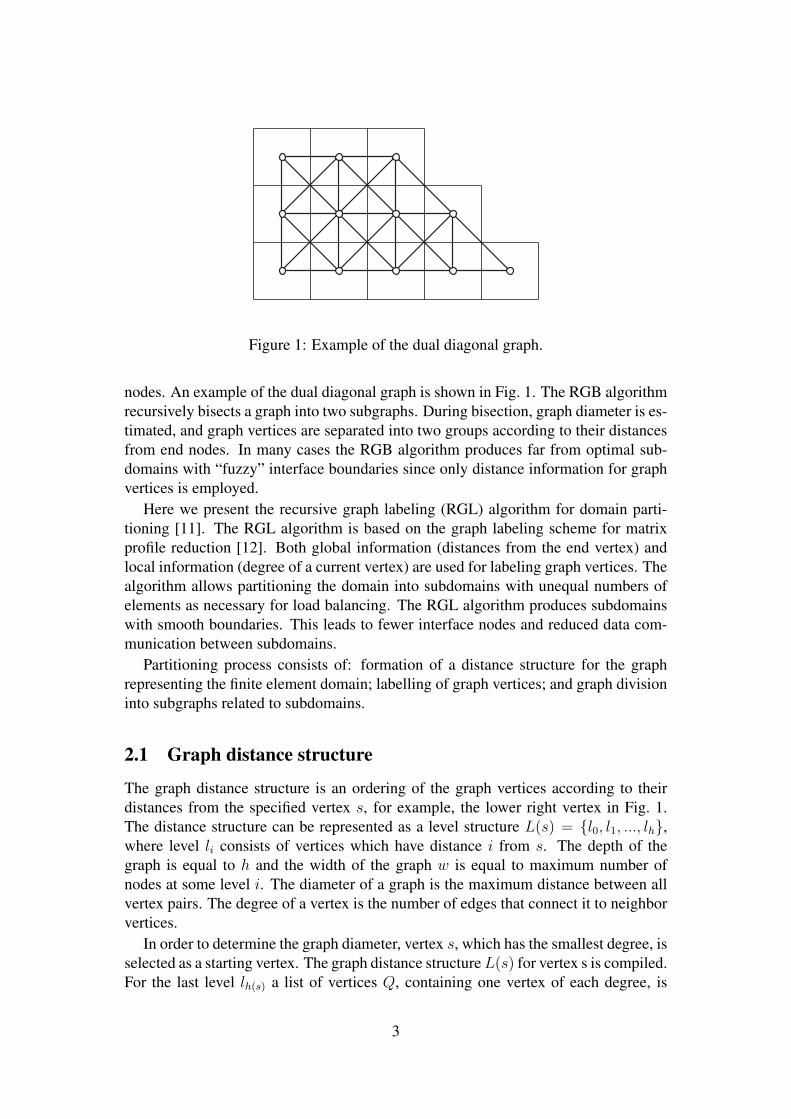
Figure 1: Example of the dual diagonal graph.

nodes. An example of the dual diagonal graph is shown in Fig. 1. The RGB algorithmrecursively bisects a graph into two subgraphs. During bisection, graph diameter is es-timated, and graph vertices are separated into two groups according to their distancesfrom end nodes. In many cases the RGB algorithm produces far from optimal sub-domains with “fuzzy” interface boundaries since only distance information for graphvertices is employed.

Here we present the recursive graph labeling (RGL) algorithm for domain parti-tioning [11]. The RGL algorithm is based on the graph labeling scheme for matrixprofile reduction [12]. Both global information (distances from the end vertex) andlocal information (degree of a current vertex) are used for labeling graph vertices. Thealgorithm allows partitioning the domain into subdomains with unequal numbers ofelements as necessary for load balancing. The RGL algorithm produces subdomainswith smooth boundaries. This leads to fewer interface nodes and reduced data com-munication between subdomains.

Partitioning process consists of: formation of a distance structure for the graphrepresenting the finite element domain; labelling of graph vertices; and graph divisioninto subgraphs related to subdomains.

2.1 Graph distance structure

The graph distance structure is an ordering of the graph vertices according to theirdistances from the specified vertex s, for example, the lower right vertex in Fig. 1.The distance structure can be represented as a level structure L(s) = {l0, l1, ..., lh},where level li consists of vertices which have distance i from s. The depth of thegraph is equal to h and the width of the graph w is equal to maximum number ofnodes at some level i. The diameter of a graph is the maximum distance between allvertex pairs. The degree of a vertex is the number of edges that connect it to neighborvertices.

In order to determine the graph diameter, vertex s, which has the smallest degree, isselected as a starting vertex. The graph distance structure L(s) for vertex s is compiled.For the last level lh(s) a list of vertices Q, containing one vertex of each degree, is

3

generated. For each vertex i in Q the distance structure L(Qi) is built. The graphdiameter is assigned the maximum depth from all h(Qi). The starting vertex s and theend vertex e are vertices at opposite ends of the diameter.

2.2 Vertex labeling

The graph labeling algorithm is based on the vertex priority, which is a combinationof the vertex degree and its distance from the end vertex

p = W1h−W2(d + 1), (1)

where W1 and W2 are weights; h is the distance from the end vertex; and d is thevertex degree. The priority of each vertix is assigned during labeling. Vertices whichare labeled are excluded from further consideration. Vertices which are adjacent tolabeled vertices are called active. Vertices adjacent to an active vertex but not active,are called preactive. All the other vertices are inactive.

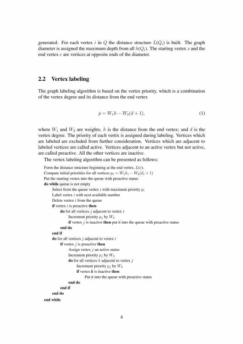
The vertex labeling algorithm can be presented as follows:

Form the distance structure beginning at the end vertex, L(e).Compute initial priorities for all vertices pi = W1hi −W2(di + 1)Put the starting vertex into the queue with preactive statusdo while queue is not empty

Select from the queue vertex i with maximum priority pi

Label vertex i with next available numberDelete vertex i from the queueif vertex i is preactive then

do for all vertices j adjacent to vertex i

Increment priority pj by W2

if vertex j is inactive then put it into the queue with preactive statusend do

end ifdo for all vertices j adjacent to vertex i

if vertex j is preactive thenAssign vertex j an active statusIncrement priority pj by W2

do for all vertices k adjacent to vertex j

Increment priority pj by W2

if vertex k is inactive thenPut it into the queue with preactive status

end doend if

end doend while

4

2.3 Division into subdomains

Suppose that the finite element domain should be partitioned into s subdomains withequal numbers of elements. Integer s is represented as a product of simple numbers s= s1 · s2 · ... · sq and the graph labeling algorithm is applied q times as shown below:

Represent the number of subdomains as s = s1 · s2 · ... · sq

Current number of subdomains N = 1do i = 1, q

do j = 1, N

Partition subdomain j into si subdomains using graph labelingIncrement the current number of subdomains N = N · si

end doend do

Partitioning of a subdomain consisting of E elements into si new equal subdomainsincludes the following steps. Using labeling, elements are sorted according to theirpriorities. First E/si elements are assigned to the first new subdomain; next E/si

elements are assigned to the second subdomain; and so on. It is not difficult to partitionthe subdomain into unequal new subdomains with specified numbers of elements.

3 Domain decomposition method with a direct solver

The DDM with subdomain condensation is called the Schur complement method[1, 2]. The finite element domain is divided into subdomains. For each subdomain,elimination of inner nodes is performed. The condensed subdomain matrices are as-sembled into an interface equation system, which solution produces interface displace-ments. Finally, inner displacements and other results like strains and stresses are com-puted.

3.1 DDM algorithm

After division of the computational domain into a number of subdomains, a finiteelement equation system can be assembled for each subdomain:

[k]{u} = {f}, (2)

where [k] is a subdomain stiffness matrix, {u} is a subdomain displacement vector,and {f} is a subdomain load vector.

The subdomain nodes are grouped into interior nodes, designated by the subscripti, and interface boundary nodes, designated by the subscript b. If the interior nodesare numbered first and the interface boundary nodes are numbered last, then the sub-domain equation system can be written in the following matrix form:

[kii kib

kbi kbb

]{ui

ub

}=

{fi

fb

}. (3)

5

Matrices [kii] and [kbb] correspond to interior and interface (boundary) nodes respec-tively. Matrix [kib] reflects the interaction between the interior and boundary nodes.A condensation of the subdomain equation system is made by eliminating unknownsrelated to interior nodes:

[kbb]{ub} = {fb},[kbb] = [kbb]− [kbi][kii]

−1[kib],{fb} = {fb} − [kbi][kii]

−1{fi}.(4)

Subdomain condensed stiffness matrices [kbb] and subdomain surface load vectors{fb} are assembled into the interface equation system

[K]{U} = {F}. (5)

Solution of the interface system gives unknown interface displacements {U}. In-terface displacements are diassembled and used for the determination of the interiordisplacements for each subdomain:

[kii]{ui} = {fi} − [kib]{ub}. (6)

Let us adopt the LDU method for subdomain condensation. The DDM numericalprocedure with the LDU subdomain condensation has three computational phases –

(a) Subdomain assembly and condensation:

[k] =∑

el

[kel], {f} =∑

el

{fel},

[kii] = [L][D][U ] = [U ]T [D][U ],[kib] = [U ]−T [kib],[kbb] = [kbb]− [kib]

T [D]−1[kib],{fi} = [U ]−T{fi},{fb} = {fb} − [kib]

T [D]−1{fi}.

(7)

(b) Interface assembly and solution:

[K] =∑

s

[kbb], {F} =∑

s

{fb},{U} = [K]−1{F}.

(8)

(c) Determination of interior displacements:

{fi} = {fi} − [kib]T{ub},

{ui} = [U ]−1[D]−1{fi}. (9)

Different subdomains are assigned to different processors for parallel computing.Subdomain stiffness matrices and subdomain load vectors are assembled of elementstiffness matrices and element load vectors. The subdomain condensation procedure

6

(7) consists of LDU factorization of the matrix [kii] with the interior degrees of free-dom and matrix-matrix and matrix-vector multiplications. Subdomain operations ofassembly and condensation take the most time and can be done in parallel without anydata communication. All parallel tasks should be synchronized at the beginning of thesolution of the interface equation system, thus the compute load for the subdomainassembly and condensation should be balanced among processors.

Optimized node enumeration inside each subdomain can substantially decrease theoperation count for the condensation of the subdomain matrices. The graph labelingalgorithm of Section 2 with necessary modifications can be used for subdomain noderenumbering. The dual diagonal graph is generated for nodes. If a subdomain has apart of the boundary which does not belong to the interface, then the starting node isplaced on that part of the boundary.

Solution of the interface equation system can be performed with direct or iterativemethods. If a direct method is used, then factorization of the interface equation sys-tem can be done in parallel [13] using cyclic distribution of matrix columns acrossprocessors. Each column after modifications is broadcast to all processors. Then eachparallel task uses the received column for modification of columns belonging to thistask. The forward solve and backsubstitution phase for the interface system is notwell suited for parallelization because of its very low computation to communicationratio. Since the backsolve takes a tiny fraction of total computing time, it is possibleto perform this operation in a serial manner. Finite element operations that followthe determination of displacements (usually stress calculations) are element-orientedand not difficult to parallelize. The distribution of elements across processors duringthe stress calculations can differ from subdomain partition used during the previouscomputational phases.

3.2 Compute load for subdomains

Analyzing the DDM computational procedure it is possible to conclude that it is im-portant to balance compute load for subdomain assembly and condensation. Beloware presented operation count estimates for this computational phase [11, 14].

The operation count for the assembly of the subdomain equation system is mainlydetermined by element stiffness calculations, and can be estimated as

c = cele, (10)

where cel is the operation count for computing the element stiffness matrix and e isthe number of elements in the subdomain. For estimation of the number of arithmeticoperations for element stiffness matrix calculation, it is possible to use the computingtime for element stiffness calculation and the average computer Mflops rate.

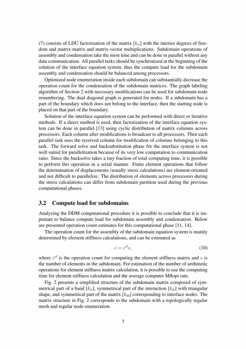
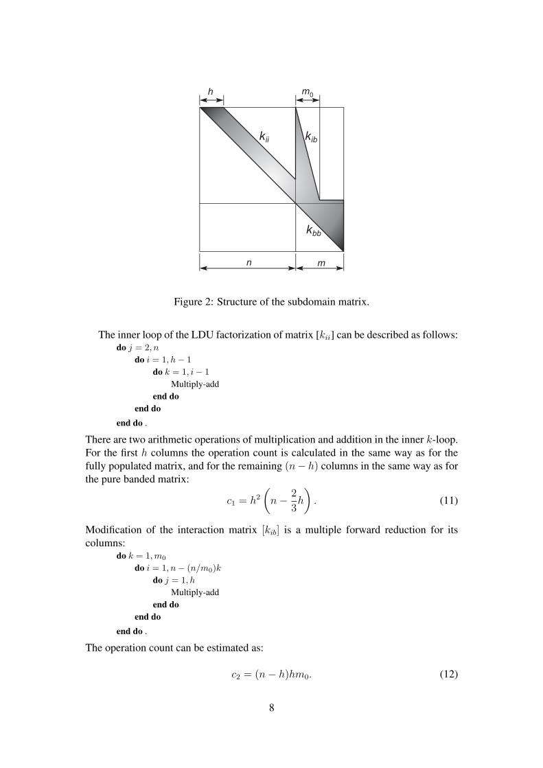
Fig. 2 presents a simplified structure of the subdomain matrix composed of sym-metrical part of a band [kii], symmetrical part of the interaction [kib] with triangularshape, and symmetrical part of the matrix [kbb] corresponding to interface nodes. Thematrix structure in Fig. 2 corresponds to the subdomain with a topologically regularmesh and regular node enumeration.

7

h m0

n m

kib

kbb

kii

Figure 2: Structure of the subdomain matrix.

The inner loop of the LDU factorization of matrix [kii] can be described as follows:do j = 2, n

do i = 1, h− 1do k = 1, i− 1

Multiply-addend do

end doend do .

There are two arithmetic operations of multiplication and addition in the inner k-loop.For the first h columns the operation count is calculated in the same way as for thefully populated matrix, and for the remaining (n− h) columns in the same way as forthe pure banded matrix:

c1 = h2

(n− 2

3h

). (11)

Modification of the interaction matrix [kib] is a multiple forward reduction for itscolumns:

do k = 1,m0

do i = 1, n− (n/m0)kdo j = 1, h

Multiply-addend do

end doend do .

The operation count can be estimated as:

c2 = (n− h)hm0. (12)

8

The fill factor f for the interaction matrix [kib] is calculated as

f =1

mn

∑m

i=1hi, (13)

where hi is the height of the ith column. For our simplified structure for the matrix[kib] with m0 = m/2, the size m0 is equal to:

m0 = 2mf

and the operation count c2 is expressed as:

c2 = 2(n− h)mhf. (14)

Calculation of the symmetric part of the condensed stiffness matrix [kbb] is a multi-plication of a profile transpose matrix [kib] by itself:

do j = 1,m

do i = 1, j

do k = 1, n− (n/m0)max(i, j)Multiply-add

end doend do

end do .

The operation count can be estimated by computing an integral

c3 =

∫ m0

0

(1

2nm0 − 1

2x2 n

m0

)dx =1

3nm2

0 =4

3nm2f 2, (15)

where x is a column number in the matrix [kib].Summing operation counts of (10), (11), (14) and (15) yields the total compute load

for assembly and condensation of the subdomain stiffness matrix:

C = cele + h2(n− 2

3h) + 2(n− h)mhf +

4

3nm2f 2. (16)

Partitioning of the finite element domain into subdomains with an equal numberof elements does not lead to interprocessor load balancing since the quantities n, m,h, and f are different in different subdomains because of the subdomain position andsubdomain node enumeration.

In actual calculations, the structure of the subdomain stiffness matrix is more com-plicated than the structure shown in Fig. 2. The operation count estimate (16) can beused for irregular subdomains provided that the halfbandwidth h is replaced by its rootmean square value:

h =

√1

n

∑n

i=1h2

i , (17)

where hi is the height of the ith column of the matrix [kii]

9

3.3 Subdomain load balancing

The first phase of the DDM algorithm is assembly and condensation of the subdomainstiffness matrices. Since the computation time for the subdomain assembly and con-densation is the largest fraction of the total solution and the end of this phase is thesynchronization point, the compute load of the subdomain assembly and condensa-tion should be balanced among processors. The load balancing may be achieved bypartitioning the domain into subdomains with unequal numbers of elements [11].

For subdomains having varying number of elements and similar shape, quantitiesof equation (16) are approximately proportional to:

n ∼ e; m ∼ √e; h ∼ √

e; f ≈ const.

The operation count for the subdomain can be expressed through the number of ele-ments

C = cele + ceqe2, (18)

where ceq is the operation count related to subdomain condensation. The value of thecoefficient ceq is determined by

ceq = (h2n + 2nmhf +4

3nm2f 2)/e2

0 (19)

for some subdomain with known values of n, h, m, and f and number of elements e0.A nonlinear equation system for the load balancing problem can be written as:

C1 − C2 = 0C2 − C3 = 0...Cs−1 − Cs = 0∑

ei − E = 0,

(20)

orcelei + ceq

i e2i − celei+1 − ceq

i+1e2i+1 = 0, i = 1...s− 1∑

ei − E = 0,(21)

where s is the number of subdomains, ei is the number of elements in the ith subdo-main, and E is the number of elements in the domain.

The nonlinear equation system (21)

Fi(e1, ...es) = 0, i = 1...s (22)

can be solved by the Newton-Raphson iterative procedure:

{e}(0) = {E/s, E/s...}{∆e}(i) = −([J ](i−1))−1{F}(i−1)

{e}(i) = {e}(i−1) + {∆e}(i).(23)

10

Here (i) is the iteration number and coefficients of the matrix [J] are equal to Jij =∂Fi/∂ej:

Ji1, ...Ji i−1 = 0Jii = cel + 2ceq

i ei

Ji i+1 = −cel − 2ceqi+1ei+1

Ji i+2, ...Jin = 0Jsi = 1.

(24)

Solution of the nonlinear load balancing system (21) predicts the new distributionof elements among subdomains. The algorithm of partitioning with load balancing isdescribed by the following pseudo-code:

Represent number of subdomains s as product of simple numbersSpecify equal number of elements in subdomains {e}(0) = {E/s,E/s...}while load imbalance ≥ specified value

Partition domain into s subdomains {e}(i−1) using recursive graph labeling methodOptimize subdomain node enumeration with minimization of h and f

Calculate {e}(i) by solving algebraic problem of element distribution among subdomains

end while .

Usually it is sufficient to perform 1–3 iterations in order to achieve acceptable loadbalancing across subdomains.

3.4 Examples

The above algorithm of domain partitioning with load balancing has been imple-mented as a C routine. Although it is not possible to prove the convergence of theiterative load balancing procedure, one can intuitively feel that the iterative procedureconverges if the subdomains undergo small changes in shape and position betweensuccessive iterations. To provide similarity of subdomains during load balancing iter-ations, the following procedure was introduced into the algorithm. During the initialpartitioning, graph diameter ends for all subdomains are stored. Later, each diam-eter end is selected as an element located at the subdomain boundary and has theminimum distance from the diameter end stored during the first partitioning. In or-der to “sharpen” subdomain boundaries, a large weight W2 for vertex degrees is used(W2 À W1) in the recursive graph labeling algorithm. Degrees for all interior ele-ments are set to the same value, which is equal to the degree of the interior element inthe regular mesh.

Here, examples of partitioning both regular and irregular meshes are presented.Partitions are evaluated in terms of parallel efficiency for subdomain assembly andcondensation computational phase. The parallel efficiency is calculated as

Ep =C(sequential, equal subdomains)

s · C(maximum among subdomains),

where s is the number of subdomains. Operation counts C both for partitions intosubdomains with equal number of elements and for optimized partitions are compared

11

(a)

(b)

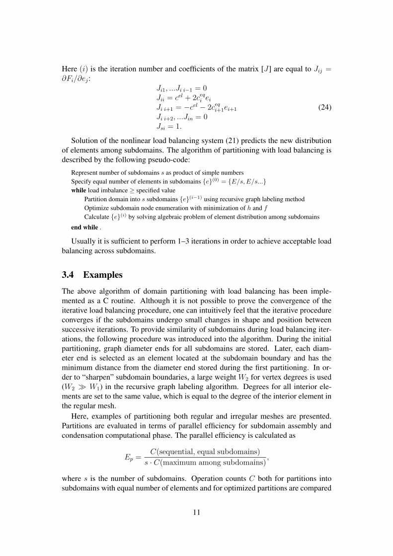
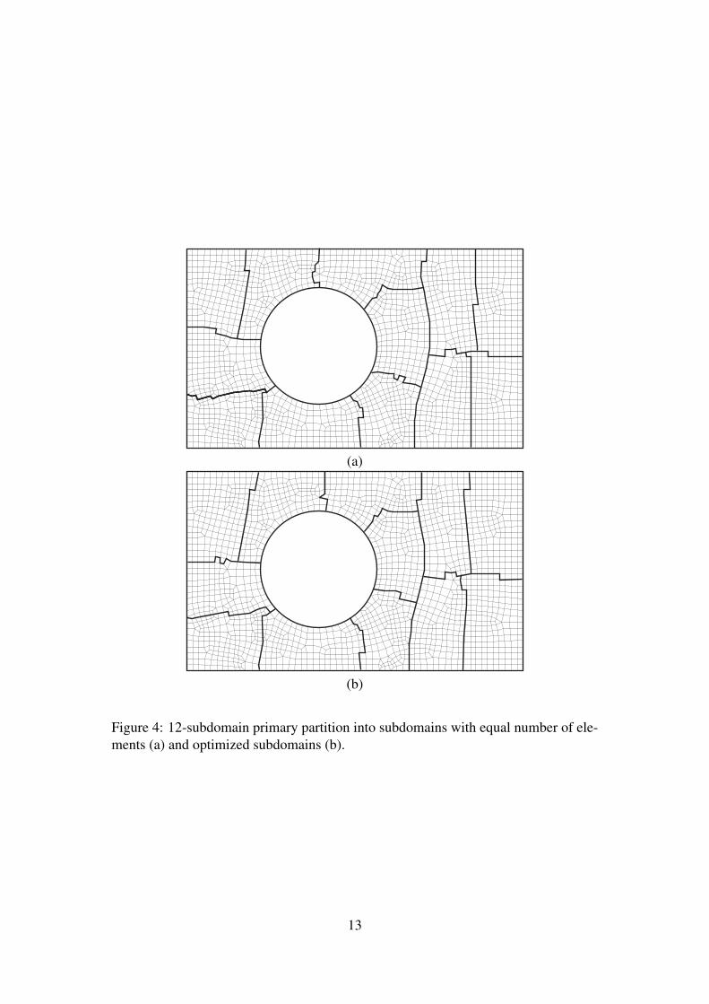
Figure 3: Eight-subdomain primary partition into equal(a) and optimized (b) subdo-mains.

to the operation count of the sequential algorithm for the partition with equal subdo-mains. Because of this, values of the parallel efficiency larger than 1.0 for optimizedsubdomains are possible. Two-dimensional four-node elements with Cel = 0.00738·106 are used in examples.

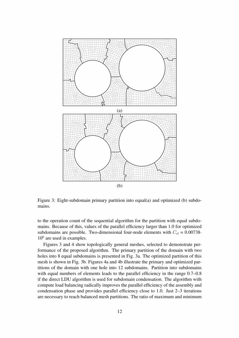
Figures 3 and 4 show topologically general meshes, selected to demonstrate per-formance of the proposed algorithm. The primary partition of the domain with twoholes into 8 equal subdomains is presented in Fig. 3a. The optimized partition of thismesh is shown in Fig. 3b. Figures 4a and 4b illustrate the primary and optimized par-titions of the domain with one hole into 12 subdomains. Partition into subdomainswith equal numbers of elements leads to the parallel efficiency in the range 0.7–0.8if the direct LDU algorithm is used for subdomain condensation. The algorithm withcompute load balancing radically improves the parallel efficiency of the assembly andcondensation phase and provides parallel efficiency close to 1.0. Just 2–3 iterationsare necessary to reach balanced mesh partitions. The ratio of maximum and minimum

12

(a)

(b)

Figure 4: 12-subdomain primary partition into subdomains with equal number of ele-ments (a) and optimized subdomains (b).

13

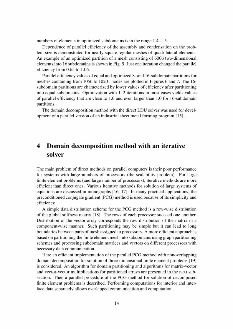
numbers of elements in optimized subdomains is in the range 1.4–1.5.Dependence of parallel efficiency of the assembly and condensation on the prob-

lem size is demonstrated for nearly square regular meshes of quadrilateral elements.An example of an optimized partition of a mesh consisting of 6006 two-dimensionalelements into 16 subdomains is shown in Fig. 5. Just one iteration changed the parallelefficiency from 0.65 to 1.06.

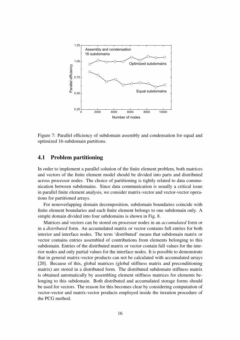
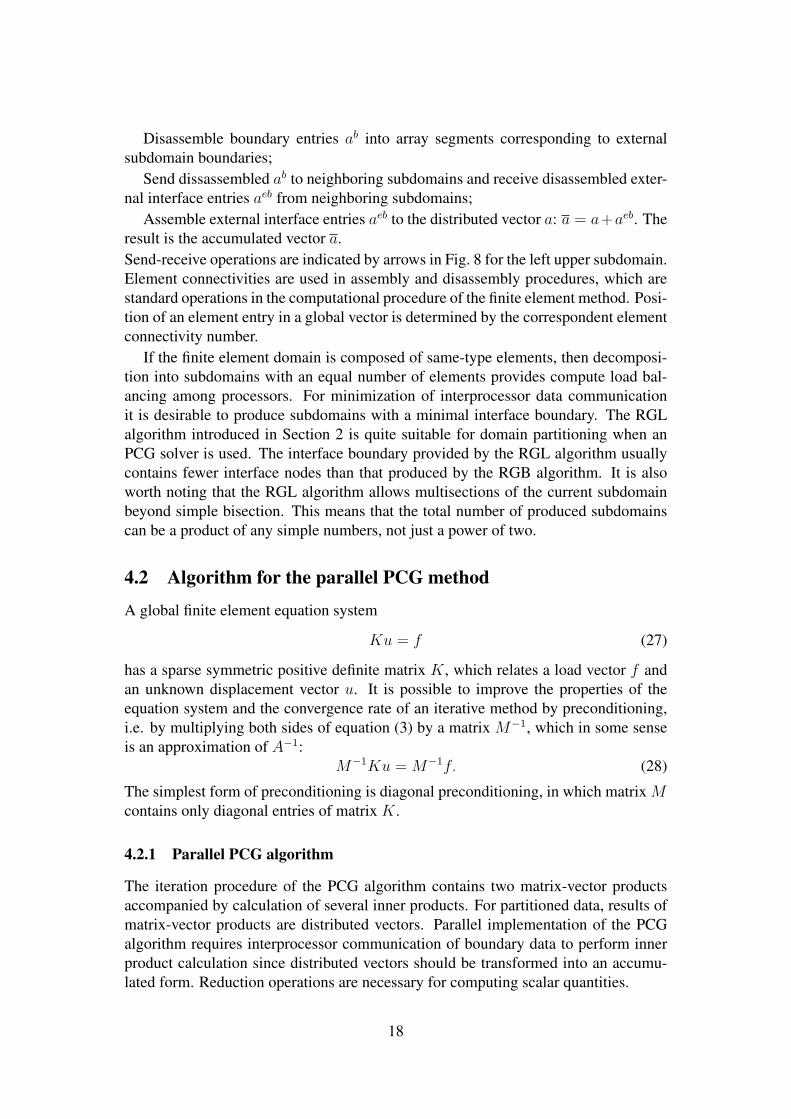
Parallel efficiency values of equal and optimized 8- and 16-subdomain partitions formeshes containing from 1056 to 10201 nodes are plotted in Figures 6 and 7. The 16-subdomain partitions are characterized by lower values of efficiency after partitioninginto equal subdomains. Optimization with 1–2 iterations in most cases yields valuesof parallel efficiency that are close to 1.0 and even larger than 1.0 for 16-subdomainpartitions.

The domain decomposition method with the direct LDU solver was used for devel-opment of a parallel version of an industrial sheet metal forming program [15].

4 Domain decomposition method with an iterativesolver

The main problem of direct methods on parallel computers is their poor performancefor systems with large numbers of processors (the scalability problem). For largefinite element problems (and large number of processors), iterative methods are moreefficient than direct ones. Various iterative methods for solution of large systems ofequations are discussed in monographs [16, 17]. In many practical applications, thepreconditioned conjugate gradient (PCG) method is used because of its simplicity andefficiency.

A simple data distribution scheme for the PCG method is a row-wise distributionof the global stiffness matrix [18]. The rows of each processor succeed one another.Distribution of the vector array corresponds the row distribution of the matrix in acomponent-wise manner. Such partitioning may be simple but it can lead to longboundaries between parts of mesh assigned to processors. A more efficient approach isbased on partitioning the finite element mesh into subdomains using graph partitioningschemes and processing subdomain matrices and vectors on different processors withnecessary data communication.

Here an efficient implementation of the parallel PCG method with nonoverlappingdomain decomposition for solution of three-dimensional finite element problems [19]is considered. An algorithm for domain partitioning and algorithms for matrix-vectorand vector-vector multiplications for partitioned arrays are presented in the next sub-section. Then a parallel procedure of the PCG method for solution of decomposedfinite element problems is described. Performing computations for interior and inter-face data separately allows overlapped communication and computation.

14

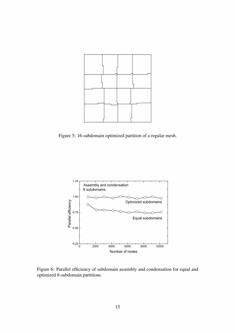
Figure 5: 16-subdomain optimized partition of a regular mesh.

0 2000 4000 6000 8000 100000.25

0.50

0.75

1.00

1.25

Optimized subdomains

Equal subdomains

8 subdomainsAssembly and condensation

Para

llel e

ffici

ency

Number of nodes

Figure 6: Parallel efficiency of subdomain assembly and condensation for equal andoptimized 8-subdomain partitions.

15

0 2000 4000 6000 8000 100000.25

0.50

0.75

1.00

1.25

Optimized subdomains

Equal subdomains

16 subdomainsAssembly and condensation

Para

llel e

ffici

ency

Number of nodes

Figure 7: Parallel efficiency of subdomain assembly and condensation for equal andoptimized 16-subdomain partitions.

4.1 Problem partitioning

In order to implement a parallel solution of the finite element problem, both matricesand vectors of the finite element model should be divided into parts and distributedacross processor nodes. The choice of partitioning is tightly related to data commu-nication between subdomains. Since data communication is usually a critical issuein parallel finite element analysis, we consider matrix-vector and vector-vector opera-tions for partitioned arrays.

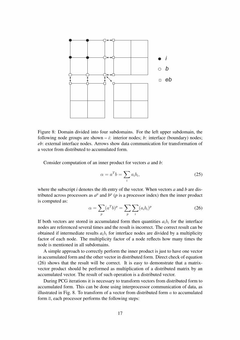
For nonoverlapping domain decomposition, subdomain boundaries coincide withfinite element boundaries and each finite element belongs to one subdomain only. Asimple domain divided into four subdomains is shown in Fig. 8.

Matrices and vectors can be stored on processor nodes in an accumulated form orin a distributed form. An accumulated matrix or vector contains full entries for bothinterior and interface nodes. The term ‘distributed’ means that subdomain matrix orvector contains entries assembled of contributions from elements belonging to thissubdomain. Entries of the distributed matrix or vector contain full values for the inte-rior nodes and only partial values for the interface nodes. It is possible to demonstratethat in general matrix-vector products can not be calculated with accumulated arrays[20]. Because of this, global matrices (global stiffness matrix and preconditioningmatrix) are stored in a distributed form. The distributed subdomain stiffness matrixis obtained automatically by assembling element stiffness matrices for elements be-longing to this subdomain. Both distributed and accumulated storage forms shouldbe used for vectors. The reason for this becomes clear by considering computation ofvector-vector and matrix-vector products employed inside the iteration procedure ofthe PCG method.

16

i

b

eb

Figure 8: Domain divided into four subdomains. For the left upper subdomain, thefollowing node groups are shown – i: interior nodes; b: interface (boundary) nodes;eb: external interface nodes. Arrows show data communication for transformation ofa vector from distributed to accumulated form.

Consider computation of an inner product for vectors a and b:

α = aT b =∑

i

aibi, (25)

where the subscript i denotes the ith entry of the vector. When vectors a and b are dis-tributed across processors as ap and bp (p is a processor index) then the inner productis computed as:

α =∑

p

(aT b)p =∑

p

∑i

(aibi)p (26)

If both vectors are stored in accumulated form then quantities aibi for the interfacenodes are referenced several times and the result is incorrect. The correct result can beobtained if intermediate results aibi for interface nodes are divided by a multiplicityfactor of each node. The multiplicity factor of a node reflects how many times thenode is mentioned in all subdomains.

A simple approach to correctly perform the inner product is just to have one vectorin accumulated form and the other vector in distributed form. Direct check of equation(26) shows that the result will be correct. It is easy to demonstrate that a matrix-vector product should be performed as multiplication of a distributed matrix by anaccumulated vector. The result of such operation is a distributed vector.

During PCG iterations it is necessary to transform vectors from distributed form toaccumulated form. This can be done using interprocessor communication of data, asillustrated in Fig. 8. To transform of a vector from distributed form a to accumulatedform a, each processor performs the following steps:

17

Disassemble boundary entries ab into array segments corresponding to externalsubdomain boundaries;

Send dissassembled ab to neighboring subdomains and receive disassembled exter-nal interface entries aeb from neighboring subdomains;

Assemble external interface entries aeb to the distributed vector a: a = a+aeb. Theresult is the accumulated vector a.Send-receive operations are indicated by arrows in Fig. 8 for the left upper subdomain.Element connectivities are used in assembly and disassembly procedures, which arestandard operations in the computational procedure of the finite element method. Posi-tion of an element entry in a global vector is determined by the correspondent elementconnectivity number.

If the finite element domain is composed of same-type elements, then decomposi-tion into subdomains with an equal number of elements provides compute load bal-ancing among processors. For minimization of interprocessor data communicationit is desirable to produce subdomains with a minimal interface boundary. The RGLalgorithm introduced in Section 2 is quite suitable for domain partitioning when anPCG solver is used. The interface boundary provided by the RGL algorithm usuallycontains fewer interface nodes than that produced by the RGB algorithm. It is alsoworth noting that the RGL algorithm allows multisections of the current subdomainbeyond simple bisection. This means that the total number of produced subdomainscan be a product of any simple numbers, not just a power of two.

4.2 Algorithm for the parallel PCG method

A global finite element equation system

Ku = f (27)

has a sparse symmetric positive definite matrix K, which relates a load vector f andan unknown displacement vector u. It is possible to improve the properties of theequation system and the convergence rate of an iterative method by preconditioning,i.e. by multiplying both sides of equation (3) by a matrix M−1, which in some senseis an approximation of A−1:

M−1Ku = M−1f. (28)

The simplest form of preconditioning is diagonal preconditioning, in which matrix Mcontains only diagonal entries of matrix K.

4.2.1 Parallel PCG algorithm

The iteration procedure of the PCG algorithm contains two matrix-vector productsaccompanied by calculation of several inner products. For partitioned data, results ofmatrix-vector products are distributed vectors. Parallel implementation of the PCGalgorithm requires interprocessor communication of boundary data to perform innerproduct calculation since distributed vectors should be transformed into an accumu-lated form. Reduction operations are necessary for computing scalar quantities.

18

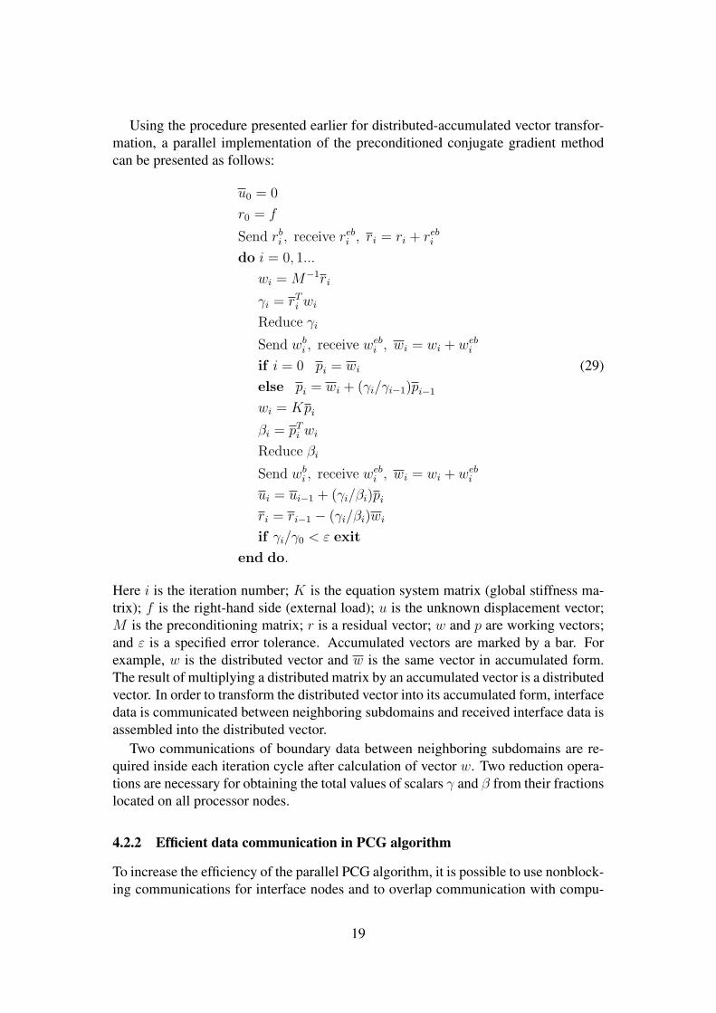
Using the procedure presented earlier for distributed-accumulated vector transfor-mation, a parallel implementation of the preconditioned conjugate gradient methodcan be presented as follows:

u0 = 0

r0 = f

Send rbi , receive reb

i , ri = ri + rebi

do i = 0, 1...

wi = M−1ri

γi = rTi wi

Reduce γi

Send wbi , receive web

i , wi = wi + webi

if i = 0 pi = wi (29)else pi = wi + (γi/γi−1)pi−1

wi = Kpi

βi = pTi wi

Reduce βi

Send wbi , receive web

i , wi = wi + webi

ui = ui−1 + (γi/βi)pi

ri = ri−1 − (γi/βi)wi

if γi/γ0 < ε exit

end do.

Here i is the iteration number; K is the equation system matrix (global stiffness ma-trix); f is the right-hand side (external load); u is the unknown displacement vector;M is the preconditioning matrix; r is a residual vector; w and p are working vectors;and ε is a specified error tolerance. Accumulated vectors are marked by a bar. Forexample, w is the distributed vector and w is the same vector in accumulated form.The result of multiplying a distributed matrix by an accumulated vector is a distributedvector. In order to transform the distributed vector into its accumulated form, interfacedata is communicated between neighboring subdomains and received interface data isassembled into the distributed vector.

Two communications of boundary data between neighboring subdomains are re-quired inside each iteration cycle after calculation of vector w. Two reduction opera-tions are necessary for obtaining the total values of scalars γ and β from their fractionslocated on all processor nodes.

4.2.2 Efficient data communication in PCG algorithm

To increase the efficiency of the parallel PCG algorithm, it is possible to use nonblock-ing communications for interface nodes and to overlap communication with compu-

19

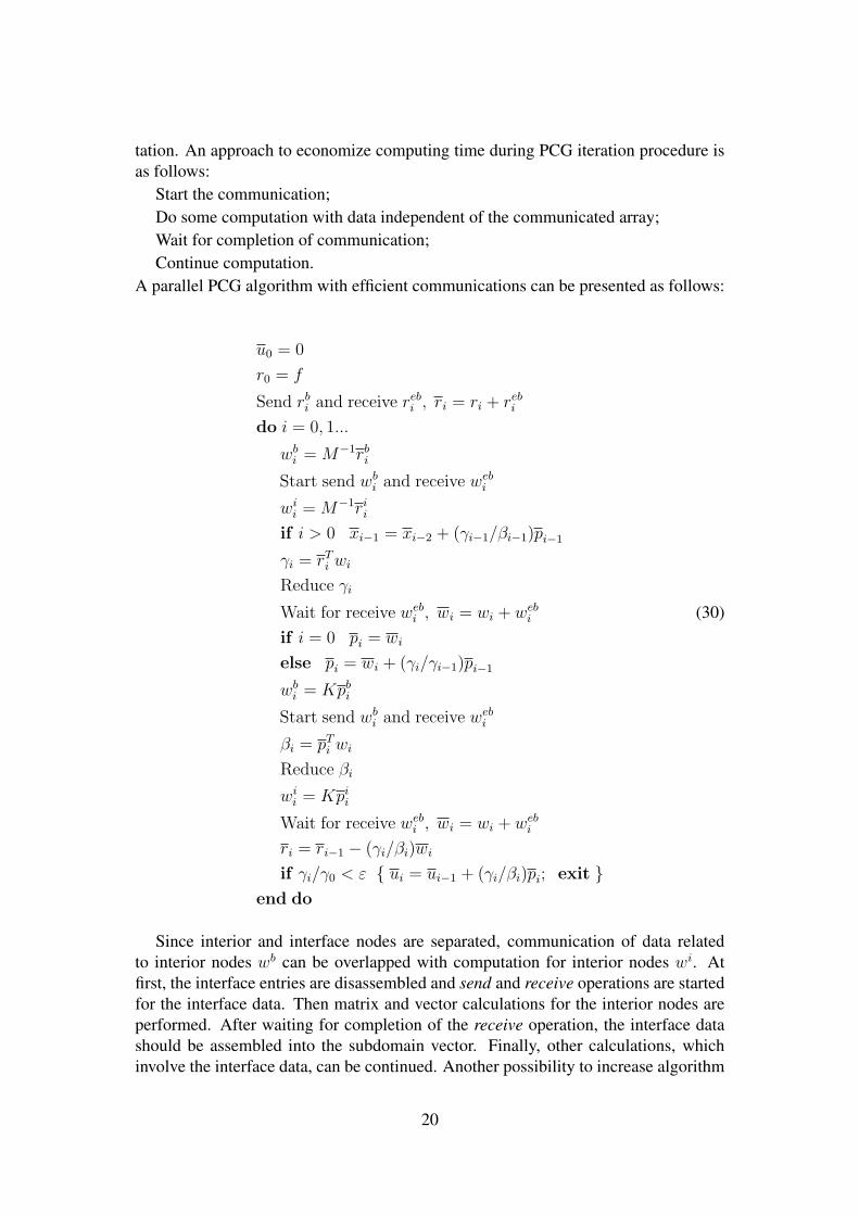
tation. An approach to economize computing time during PCG iteration procedure isas follows:

Start the communication;Do some computation with data independent of the communicated array;Wait for completion of communication;Continue computation.

A parallel PCG algorithm with efficient communications can be presented as follows:

u0 = 0

r0 = f

Send rbi and receive reb

i , ri = ri + rebi

do i = 0, 1...

wbi = M−1rb

i

Start send wbi and receive web

i

wii = M−1ri

i

if i > 0 xi−1 = xi−2 + (γi−1/βi−1)pi−1

γi = rTi wi

Reduce γi

Wait for receive webi , wi = wi + web

i (30)if i = 0 pi = wi

else pi = wi + (γi/γi−1)pi−1

wbi = Kpb

i

Start send wbi and receive web

i

βi = pTi wi

Reduce βi

wii = Kpi

i

Wait for receive webi , wi = wi + web

i

ri = ri−1 − (γi/βi)wi

if γi/γ0 < ε { ui = ui−1 + (γi/βi)pi; exit }end do

Since interior and interface nodes are separated, communication of data relatedto interior nodes wb can be overlapped with computation for interior nodes wi. Atfirst, the interface entries are disassembled and send and receive operations are startedfor the interface data. Then matrix and vector calculations for the interior nodes areperformed. After waiting for completion of the receive operation, the interface datashould be assembled into the subdomain vector. Finally, other calculations, whichinvolve the interface data, can be continued. Another possibility to increase algorithm

20

0 10 20 300

10

20

304096 20-node elements

Fixe

d si

ze s

peed

up

Number of processors

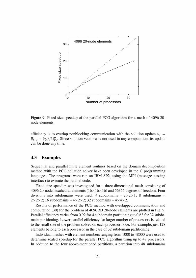
Figure 9: Fixed size speedup of the parallel PCG algorithm for a mesh of 4096 20-node elements.

efficiency is to overlap nonblocking communication with the solution update ui =ui−1 + (γi/βi)pi. Since solution vector u is not used in any computation, its updatecan be done any time.

4.3 Examples

Sequential and parallel finite element routines based on the domain decompositionmethod with the PCG equation solver have been developed in the C programminglanguage. The programs were run on IBM SP2, using the MPI (message passinginterface) to execute the parallel code.

Fixed size speedup was investigated for a three-dimensional mesh consisting of4096 20-node hexahedral elements (16×16×16) and 56355 degrees of freedom. Fourdivisions into subdomains were used: 4 subdomains = 2×2×1; 8 subdomains =2×2×2; 16 subdomains = 4×2×2; 32 subdomains = 4×4×2.

Results of performance of the PCG method with overlapped communication andcomputation (30) for the problem of 4096 3D 20-node elements are plotted in Fig. 9.Parallel efficiency varies from 0.92 for 4 subdomain partitioning to 0.63 for 32 subdo-main partitioning. Lower parallel efficiency for larger number of processors is relatedto the small size of the problem solved on each processor node. For example, just 128elements belong to each processor in the case of 32 subdomain partitioning.

Individual meshes with element numbers ranging from 1000 to 48000 were used todetermine scaled speedup for the parallel PCG algorithm using up to 48 processors.In addition to the four above-mentioned partitions, a partition into 48 subdomains

21

0 10 20 30 40 500

10

20

30

40

50

1000 20-node elements per processor

Sca

led

spee

dup

Number of processors

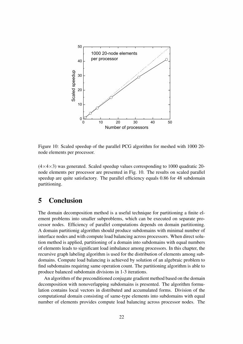
Figure 10: Scaled speedup of the parallel PCG algorithm for meshed with 1000 20-node elements per processor.

(4×4×3) was generated. Scaled speedup values corresponding to 1000 quadratic 20-node elements per processor are presented in Fig. 10. The results on scaled parallelspeedup are quite satisfactory. The parallel efficiency equals 0.86 for 48 subdomainpartitioning.

5 Conclusion

The domain decomposition method is a useful technique for partitioning a finite el-ement problems into smaller subproblems, which can be executed on separate pro-cessor nodes. Efficiency of parallel computations depends on domain partitioning.A domain partitionig algorithm should produce subdomains with minimal number ofinterface nodes and with compute load balancing across processors. When direct solu-tion method is applied, partitioning of a domain into subdomains with equal numbersof elements leads to significant load imbalance among processors. In this chapter, therecursive graph labeling algorithm is used for the distribution of elements among sub-domains. Compute load balancing is achieved by solution of an algebraic problem tofind subdomains requiring same operation count. The partitioning algorithm is able toproduce balanced subdomain divisions in 1-3 iterations.

An algorithm of the preconditioned conjugate gradient method based on the domaindecomposition with nonoverlapping subdomains is presented. The algorithm formu-lation contains local vectors in distributed and accumulated forms. Division of thecomputational domain consisting of same-type elements into subdomains with equalnumber of elements provides compute load balancing across processor nodes. The

22

efficient implementation of the parallel PCG algorithm uses nonblocking communica-tions for interface nodes and overlapping of communication with computation.

References

[1] J.S. Przemieniecki, “Matrix structural analysis of substructures”, AIAA Journal,1, 138-147, 1963.

[2] I. Babuska and H.C. Elman, “Some aspects of parallel implementation of thefinite-element method on message passing architectures”, Journal of Computa-tional and Applied Mathematics, 27, 157-187, 1989.

[3] K. Schloegel, G. Karypis and V. Kumar, “Graph partitioning for high per-formance scientific simulations”, CRPC Parallel Computing Handbook, MorganKaufmann, 2001.

[4] C. Farhat, “A simple and efficient automatic FEM domain decomposer”, Com-puters and Structures, 28, 579-602, 1988.

[5] H.D. Simon, “Partitioning of unstructured problems for parallel processing”,Computing Systems in Engineering, 2, 135-148, 1991.

[6] Y.F. Hu and R.J. Blake, “Numerical experiences with partitioning of unstructuredmeshes”, Parallel Computing, 20, 815-829, 1994.

[7] S. Gupta and M.R. Ramirez, “A mapping algorithm for domain decomposition inmassively parallel finite element analysis”, Computing Systems in Engineering, 6,111-150, 1995.

[8] C. Farhat, N. Maman and G.W. Brown, “Mesh partitioning for implicit compu-tations via iterative domain decomposition: impact and optimization of the subdo-main aspect ratio”, International Journal for Numerical Methods in Engineering,38, 989-1000, 1995.

[9] D. Vanderstraeten and R. Keunings, “Optimized partitioning of unstructured finiteelement meshes”, International Journal for Numerical Methods in Engineering, 38,433-450, 1995.

[10] C.H. Walshaw, M. Cross and M.G. Everett, “A localized algorithm for optimiz-ing unstructured mesh partitions”, International Journal for Supercomputer Appli-cations, 9, 280-295, 1995.

[11] G.P. Nikishkov, A. Makinouchi, G. Yagawa and S. Yoshimura, “An algorithmfor domain partitioning with load balancing”, Engineering Computations, 16,120-135, 1999.

[12] S.W. Sloan, “A FORTRAN program for profile and wavefront reduction”, Inter-national Journal for Numerical Methods in Engineering, 28, 2651-2679, 1989.

23

[13] C. Farhat and E. Wilson, “A parallel active column equation solver”, Computersand Structures, 28, 289-304, 1988.

[14] G.P. Nikishkov, A. Makinouchi, G. Yagawa and S. Yoshimura, “Performancestudy of the domain decomposition method with direct equation solver for parallelfinite element analysis”, Computational Mechanics, 19, 84-93, 1996.

[15] G.P. Nikishkov, M. Kawka, A. Makinouchi, G. Yagawa and S. Yoshimura, “Port-ing an industrial sheet metal forming code to a distributed memory parallel com-puter”, Computers and Structures, 67, 439-449, 1998.

[16] Y. Saad, Iterative methods for sparse linear systems, PWS Publishing, Boston,1996, 447 pp.

[17] O. Axelsson, Iterative solution methods, Cambridge University Press, 1996, 654pp.

[18] A. Basermann, B. Reichel and C. Schelthoff, “Preconditioned CG methods forsparse matrices on massively parallel machines”, Parallel Computing, 23, 381-398, 1997.

[19] G.P. Nikishkov and A. Makinouchi, “Parallel implementation of the PCGmethod with nonoverlapping finite element domain decomposition”, Parallel andDistributed Computing Systems, ISCA 12th Int. Conf., Fort Lauderdale, FL, USA,Aug. 18-20, 1999 (Ed. S. Olariu and J. Wu), ISCA, 540-545, 1999.

[20] G. Haase, “New matrix-by-vector multiplications based on nonoverlapping do-main decomposition data distribution”, Lecture Notes in Computer Science 1300,726-733, 1997.

24