Expenditure and output

Saving, Consumption and Investment in the Economy

Aggregate Output / Income

Recall the national income accounting identity:

Y = C + I + G + (X – M)

• From the identity, Y represents Gross Domestic Product (GDP).

• We know that GDP accounts for the goods and services

supplied in the economy over a given period.

• From a different perspective, GDP also accounts for all the

income received by the factors of production in a given period.

• Thus, to simplify, Y is a variable that measures both aggregate

output and aggregate income.

A look back at GDP and what it means.

Simplifications

• Recall that all variables are aggregates.

• Since people only care about the “real” value of their

income/output, we can assume that all variables under

consideration are expressed in real terms.

• To proceed with the analysis, we can consider the simplest

case:

• There is no government intervention in the economy

(i.e. G = 0).

• A closed economy model (i.e. [X – M] = 0).

• Thus, our model reduces to:

Y = C + I

Some assumptions to make the analysis easier.

Consumption

Determinants of aggregate consumption:

1. Household Income

2. Household Wealth

3. Households’ Expectations about the Future

4. Interest Rates

Identifying the factors that influence spending behavior.

Consumption Behavior

• Based on our simplified model, we can say that

consumption is a function of income:

C = f(Y)

• More specifically, the relationship between consumption

and income can be modeled as follows:

The Keynesian consumption function.

C = a + bY

where a = autonomous consumption

b = marginal propensity to consume (MPC)

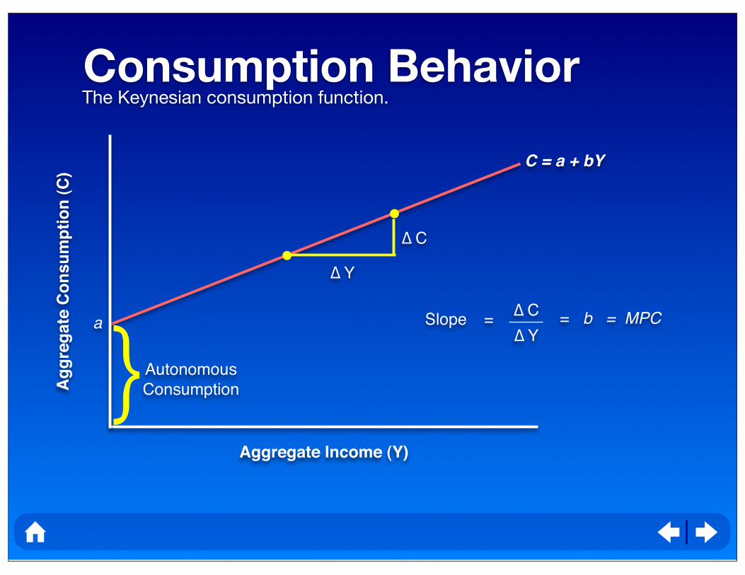
C = a + bY

Consumption BehaviorThe Keynesian consumption function.

Ag

gre

gate

Co

nsu

mp

tio

n (

C)

Aggregate Income (Y)

a

}Autonomous

Consumption

∆ C

∆ Y

= b = MPC∆ C

∆ YSlope =

Saving ≠ Savings

• Saving refers to the amount from this period’s income that

has not been spent.

• It is a flow variable and may vary from period to period.

• Savings refers to the total amount that households have

saved over their lifetimes.

• It is a stock variable that totals saving from day zero to

the present.

A little note on terminology (and a lot of nitpicking).

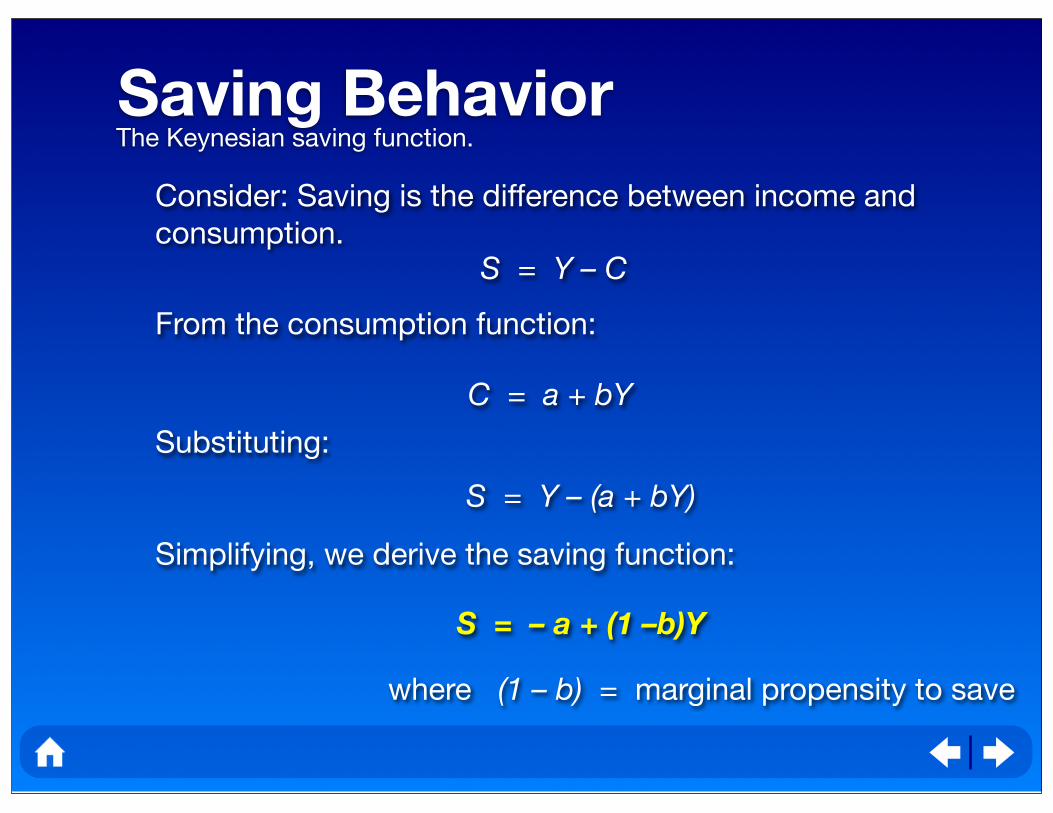
Saving BehaviorThe Keynesian saving function.

Consider: Saving is the difference between income and

consumption.S = Y – C

From the consumption function:

C = a + bY

Substituting:

S = Y – (a + bY)

Simplifying, we derive the saving function:

S = – a + (1 –b)Y

where (1 – b) = marginal propensity to save

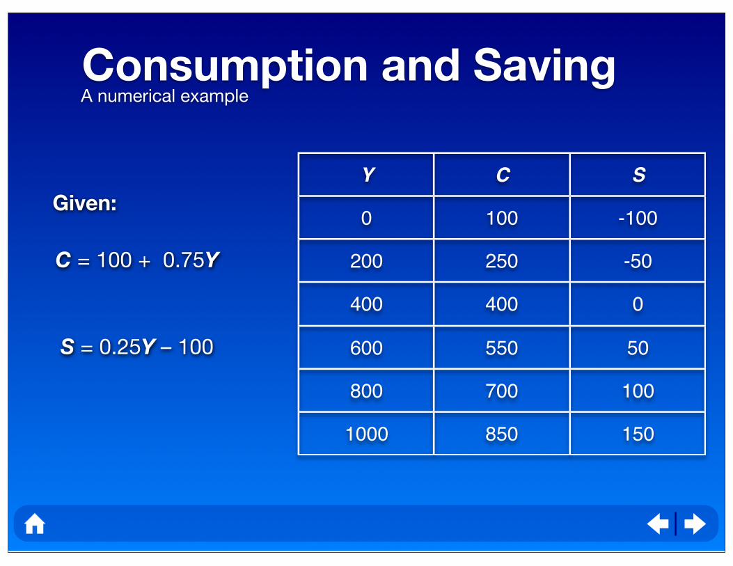
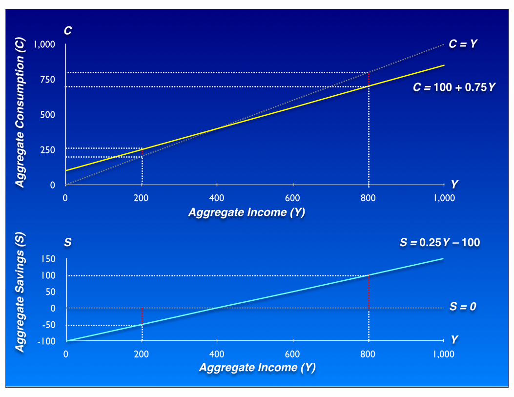
Consumption and SavingA numerical example

Y

0

200

400

600

800

1000

C

100

250

400

550

700

850

S

-100

-50

0

50

100

150

Given:

C = 100 + 0.75Y

S = 0.25Y – 100

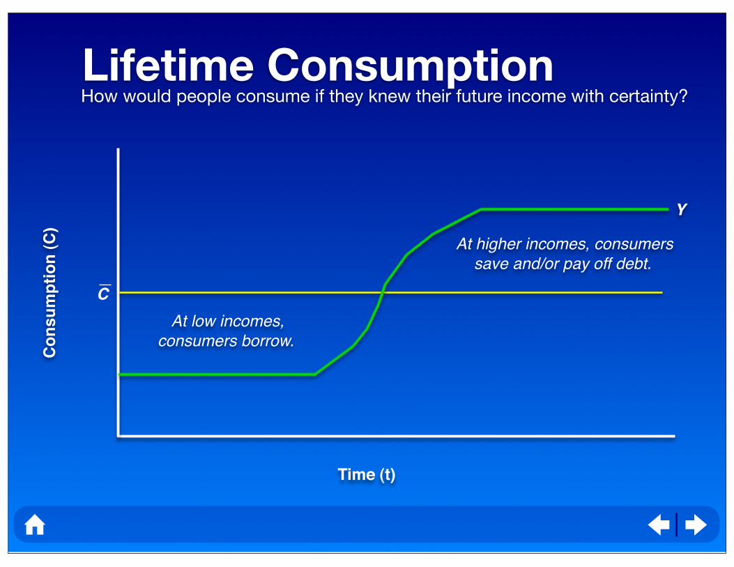
At low incomes, consumers borrow.

Lifetime ConsumptionHow would people consume if they knew their future income with certainty?

Co

nsu

mp

tio

n (

C)

Time (t)

C

Y

At higher incomes, consumers save and/or pay off debt.

0

250

500

750

1,000

0 200 400 600 800 1,000

-100

-50

0

50

100

150

0 200 400 600 800 1,000

YAgg

rega

te C

onsu

mpt

ion

(C)

S

Y

C = YC

Agg

rega

te S

avin

gs (S

)

Aggregate Income (Y)

Aggregate Income (Y)

C = 100 + 0.75Y

S = 0.25Y – 100

S = 0

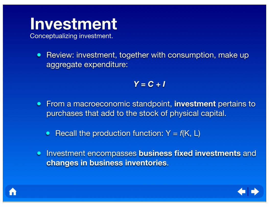
Investment

• Review: investment, together with consumption, make up

aggregate expenditure:

Y = C + I

• From a macroeconomic standpoint, investment pertains to

purchases that add to the stock of physical capital.

• Recall the production function: Y = f(K, L)

• Investment encompasses business fixed investments and

changes in business inventories.

Conceptualizing investment.

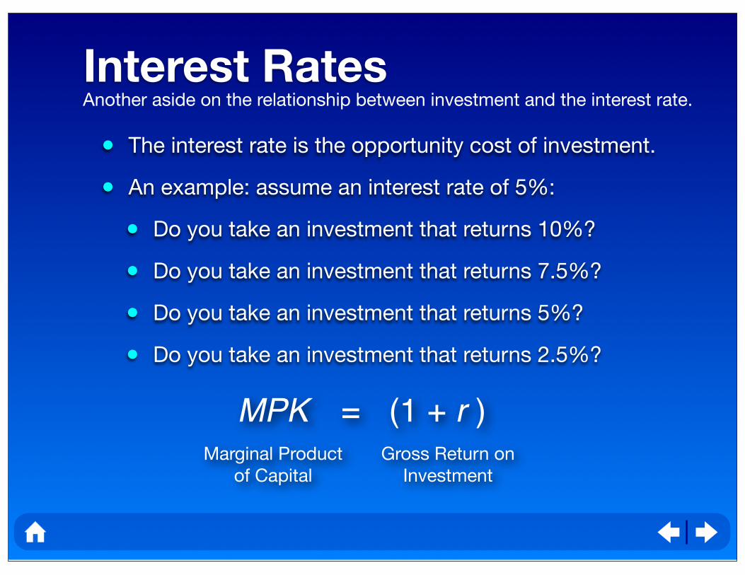
Interest Rates

• The interest rate is the opportunity cost of investment.

• An example: assume an interest rate of 5%:

• Do you take an investment that returns 10%?

• Do you take an investment that returns 7.5%?

• Do you take an investment that returns 5%?

• Do you take an investment that returns 2.5%?

Another aside on the relationship between investment and the interest rate.

MPK = (1 + r )Marginal Product

of Capital

Gross Return on

Investment

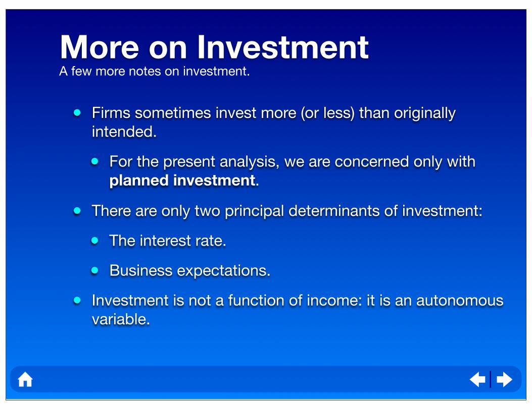
More on Investment

• Firms sometimes invest more (or less) than originally

intended.

• For the present analysis, we are concerned only with

planned investment.

• There are only two principal determinants of investment:

• The interest rate.

• Business expectations.

• Investment is not a function of income: it is an autonomous

variable.

A few more notes on investment.

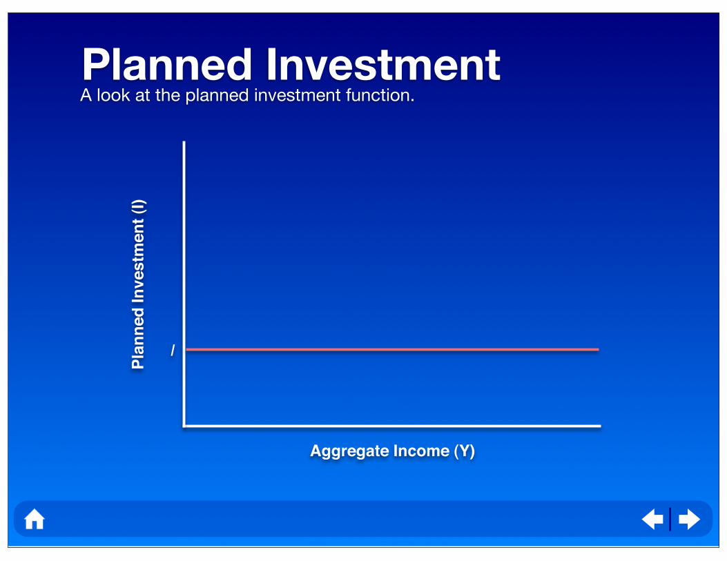
Planned InvestmentA look at the planned investment function.

Pla

nn

ed

In

vestm

en

t (I

)

Aggregate Income (Y)

I

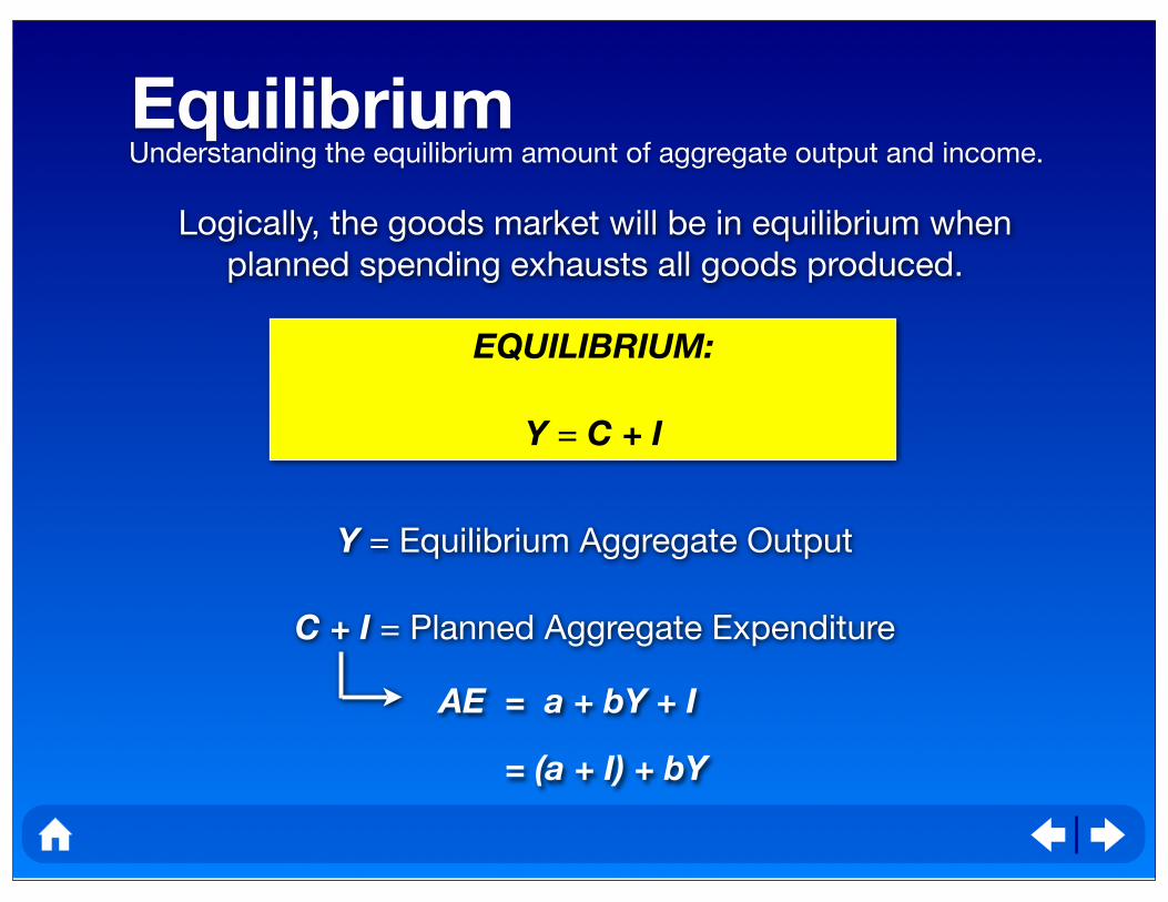
EquilibriumUnderstanding the equilibrium amount of aggregate output and income.

Logically, the goods market will be in equilibrium when

planned spending exhausts all goods produced.

Y = Equilibrium Aggregate Output

C + I = Planned Aggregate Expenditure

EQUILIBRIUM:

Y = C + I

AE = a + bY + I

= (a + I) + bY

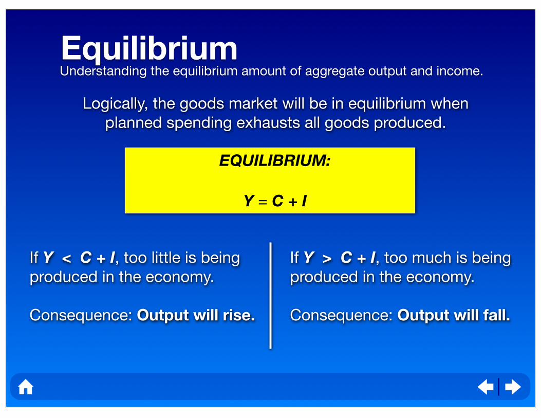
EquilibriumUnderstanding the equilibrium amount of aggregate output and income.

Logically, the goods market will be in equilibrium when

planned spending exhausts all goods produced.

If Y > C + I, too much is being

produced in the economy.

Consequence: Output will fall.

EQUILIBRIUM:

Y = C + I

If Y < C + I, too little is being

produced in the economy.

Consequence: Output will rise.

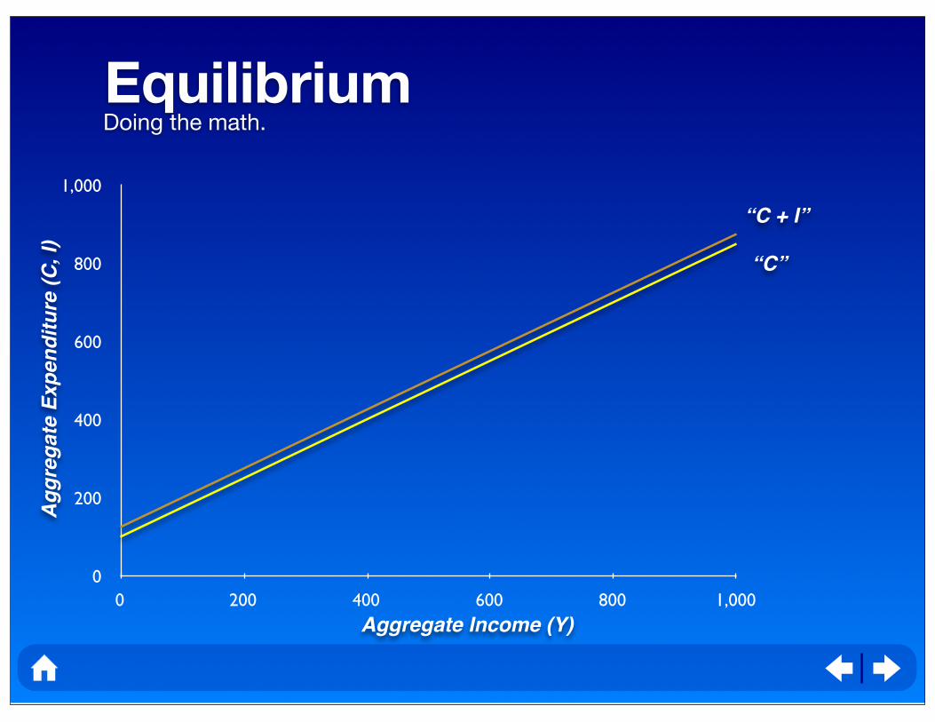
EquilibriumDoing the math.

0

200

400

600

800

1,000

0 200 400 600 800 1,000

“C + I”

Aggregate Income (Y)

Agg

rega

te E

xpen

ditu

re (C

, I)

“C”

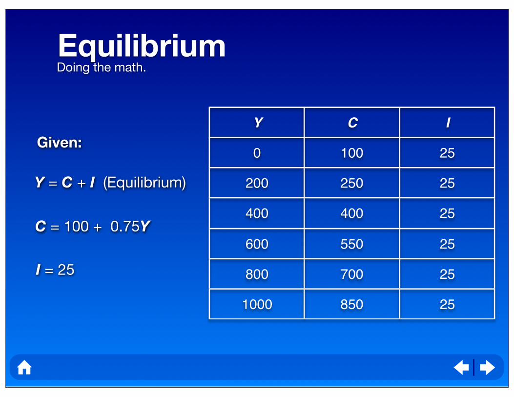
EquilibriumDoing the math.

Y C I

0 100 25

200 250 25

400 400 25

600 550 25

800 700 25

1000 850 25

Given:

Y = C + I (Equilibrium)

C = 100 + 0.75Y

I = 25

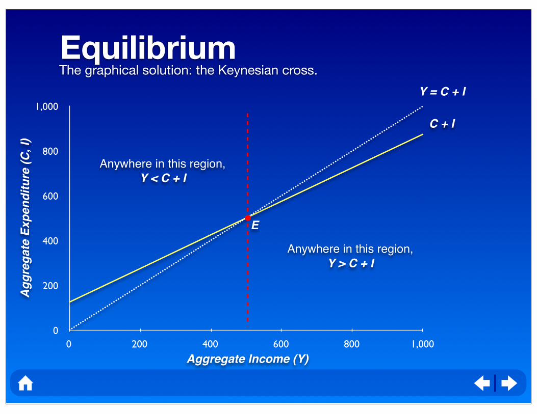
EquilibriumThe graphical solution: the Keynesian cross.

0

200

400

600

800

1,000

0 200 400 600 800 1,000

C + I

Anywhere in this region,

Y < C + I

Anywhere in this region,

Y > C + I

Y = C + I

Aggregate Income (Y)

Agg

rega

te E

xpen

ditu

re (C

, I)

E

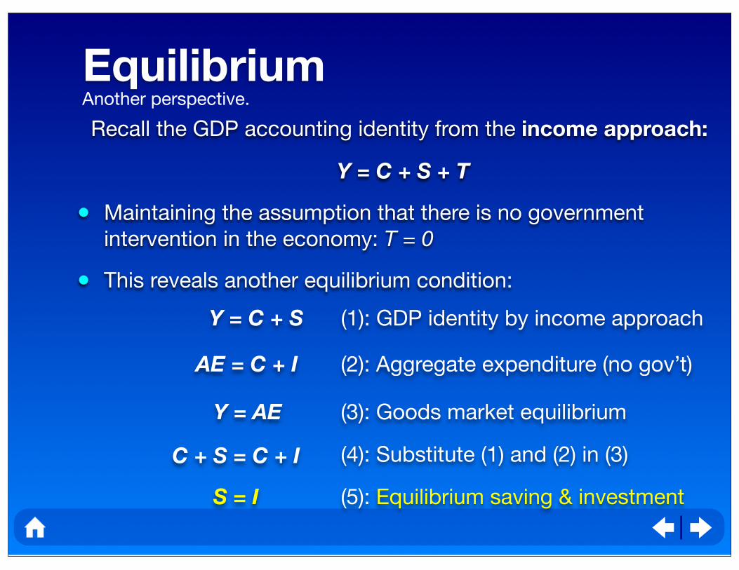
Equilibrium

Recall the GDP accounting identity from the income approach:

Y = C + S + T

• Maintaining the assumption that there is no government

intervention in the economy: T = 0

• This reveals another equilibrium condition:

Another perspective.

Y = C + S (1): GDP identity by income approach

AE = C + I (2): Aggregate expenditure (no gov’t)

Y = AE (3): Goods market equilibrium

C + S = C + I (4): Substitute (1) and (2) in (3)

S = I (5): Equilibrium saving & investment

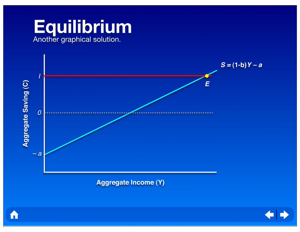
EquilibriumAnother graphical solution.

Ag

gre

gate

Savin

g (

C)

Aggregate Income (Y)

– a

S = (1-b)Y – a

0

IE

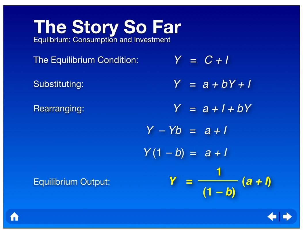
The Story So FarEquilbrium: Consumption and Investment

The Equilibrium Condition: Y = C + I

Rearranging:

Substituting: Y = a + bY + I

Y = a + I + bY

Y = (a + I) (1 – b)

1

Y – Yb = a + I

Y (1 – b) = a + I

Equilibrium Output:

What if...?

• An economy’s equilibrium output is determined by the

consumption and investment behavior of households and

firms.

• If that behavior changes, then equilibrium output will also

change.

• An increase in the economy-wide propensity to consume

also increases the amount of equilibrium output.

• An increase in the standard of living or in the amount of

investment also increases the amount of equilibrium

output, but by some multiple of the initial increase.

...things change?

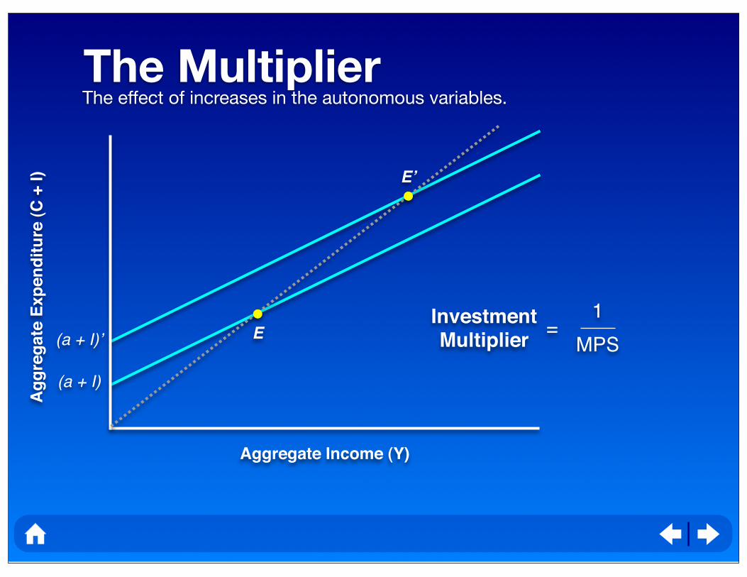
Ag

gre

gate

Exp

en

dit

ure

(C

+ I)

Aggregate Income (Y)

(a + I)

E(a + I)’

E’

The MultiplierThe effect of increases in the autonomous variables.

InvestmentMultiplier

=1

MPS

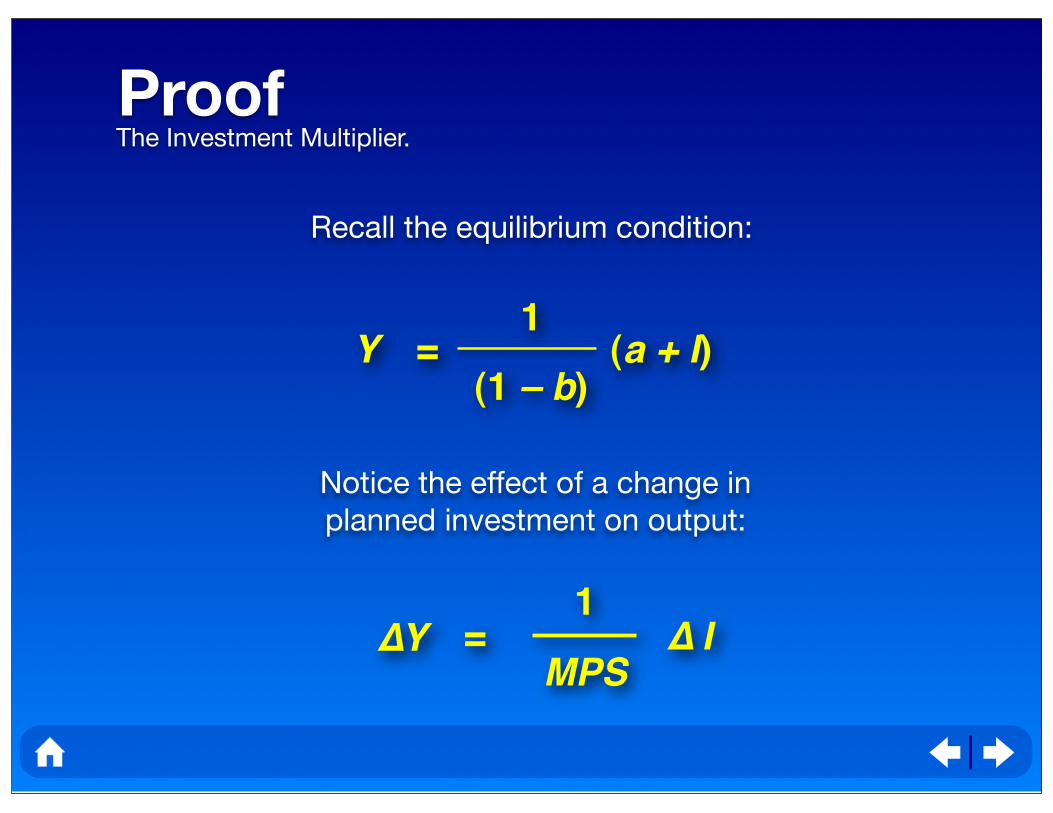
ProofThe Investment Multiplier.

Y = (a + I) (1 – b)

1

Recall the equilibrium condition:

Notice the effect of a change in

planned investment on output:

∆Y =1

MPS∆ I

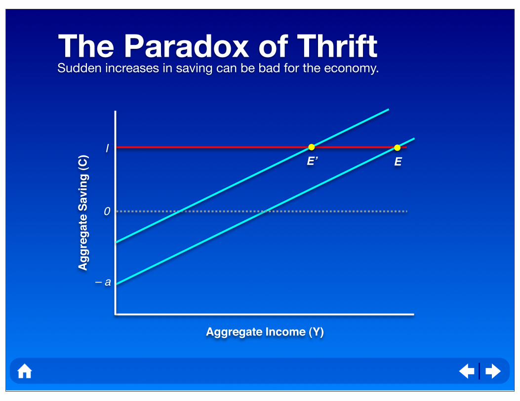
The Paradox of ThriftSudden increases in saving can be bad for the economy.

Ag

gre

gate

Savin

g (

C)

Aggregate Income (Y)

– a

0

IEE’