Chap008 lecture

08/26/2013

1

Monopoly, Oligopoly, and Monopolistic Competition

Chapter 8

Copyright © 2013 by The McGraw-Hill Companies, Inc. All rights reserved.McGraw-Hill/Irwin

8-2

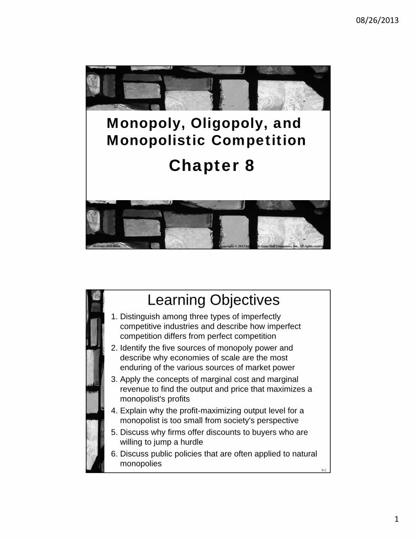
Learning Objectives1. Distinguish among three types of imperfectly

competitive industries and describe how imperfect competition differs from perfect competition

2. Identify the five sources of monopoly power and describe why economies of scale are the most enduring of the various sources of market power

3. Apply the concepts of marginal cost and marginal revenue to find the output and price that maximizes a monopolist's profits

4. Explain why the profit-maximizing output level for a monopolist is too small from society's perspective

5. Discuss why firms offer discounts to buyers who are willing to jump a hurdle

6. Discuss public policies that are often applied to natural monopolies

08/26/2013

2

8-3

Imperfect Competition

• Imperfectly competitive firms have some ability to set their own price: they are price setters– Long-run economic profits possible

– Reduce economic surplus

• Three types: 1. Monopoly has only one seller, no close

substitutes

2. Monopolistic competition has many firms producing slightly differentiated products that are reasonably close substitutes

3. Oligopoly has a small number of large firms producing products that are close substitutes

8-4

Monopolistic Competition

Monopolistic Competition

Number of Firms

Many firms

Price Limited flexibility

Entry and Exit Free

Product Differentiated

Economic Profits

Zero in long run

DecisionsP, Q, product differentiation

Perfect Competition

Many firms

Price taker

Free

Standardized

Zero in long run

Q only

08/26/2013

3

8-5

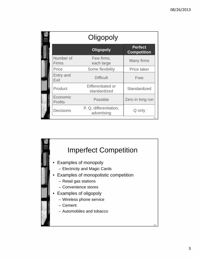
Oligopoly

Oligopoly

Number of Firms

Few firms, each large

Price Some flexibility

Entry and Exit

Difficult

ProductDifferentiated or

standardized

Economic Profits

Possible

DecisionsP, Q, differentiation,

advertising

Perfect Competition

Many firms

Price taker

Free

Standardized

Zero in long run

Q only

8-6


• Examples of monopoly– Electricity and Magic Cards

• Examples of monopolistic competition– Retail gas stations

– Convenience stores

• Examples of oligopoly– Wireless phone service

– Cement

– Automobiles and tobacco

08/26/2013

4

8-7

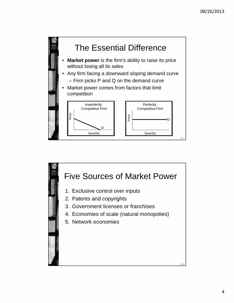
The Essential Difference• Market power is the firm's ability to raise its price

without losing all its sales

• Any firm facing a downward sloping demand curve

– Firm picks P and Q on the demand curve

• Market power comes from factors that limit competition

Quantity

Pri

ce

Imperfectly Competitive Firm

D

Quantity

Pri

ce

Perfectly Competitive Firm

D

8-8

Five Sources of Market Power

1. Exclusive control over inputs

2. Patents and copyrights

3. Government licenses or franchises

4. Economies of scale (natural monopolies)

5. Network economies

08/26/2013

5

8-9

Market Power: Economies of Scale

• Returns to scale refers to the percentage change in output from a given percentage change in ALL inputs

– Long-run idea

– Constant returns to scale: doubling all inputs doubles output

– Increasing returns to scale: output increases by a greater percentage than the increase in inputs• Average costs decrease as output increases

• Natural monopoly: a monopoly that results from economies of scale

8-10

Market Power: Network Economies

• Network economies occur when the value of the product increases as the number of users increases– VHS format for video tapes, Blu-ray for DVDs

– Telephones

– Windows operating system

– eBay

– Facebook and MySpace

08/26/2013

6

8-11

Economies of Scale and Start-Up Costs

• New products can have a large fixed development cost

• Variable cost: sum of payments made to the variable factors, such as labor

• Fixed cost: sum of payments made to the fixed factors, such as capital

• Start-up costs can be thought of as a fixed cost

• Average total cost (ATC): total cost divided by output

• A good whose production has a large start-up cost and low variable cost is subject to economies of scale

– ATC declines sharply as output increases

8-12

Economies of Scale and Start-Up Costs

• Consider an example:

• Assume marginal cost (M) is constant

• Variable cost is M*Q

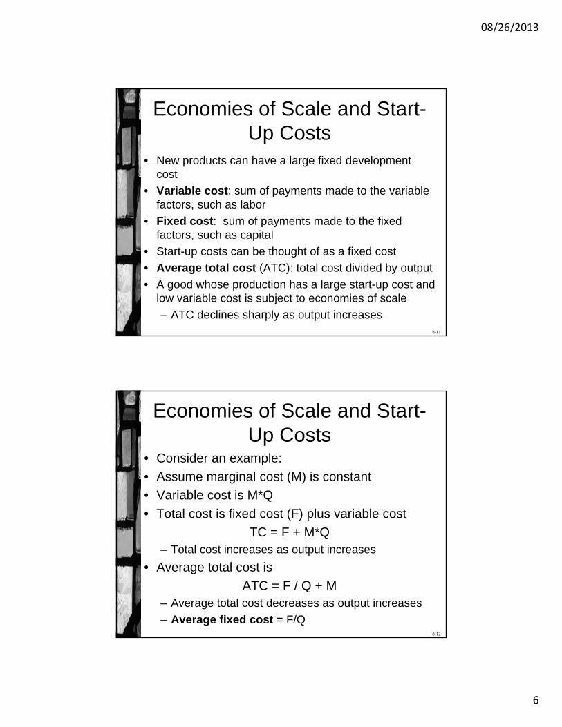
• Total cost is fixed cost (F) plus variable cost

TC = F + M*Q– Total cost increases as output increases

• Average total cost is

ATC = F / Q + M– Average total cost decreases as output increases

– Average fixed cost = F/Q

08/26/2013

7

8-13

Economies of Scale

Quantity

Tota

l cos

t ($/

year

)

F

TC = F + M Q

Ave

rage

cos

t ($/

unit)

Quantity

ATC = F/Q + M

M

8-14

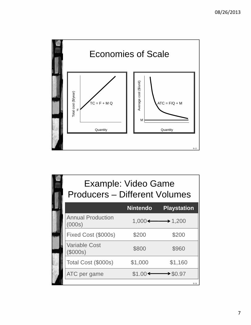
Example: Video Game Producers – Different Volumes

Nintendo Playstation

Annual Production (000s)

1,000 1,200

Fixed Cost ($000s) $200 $200

Variable Cost ($000s)

$800 $960

Total Cost ($000s) $1,000 $1,160

ATC per game $1.00 $0.97

08/26/2013

8

8-15

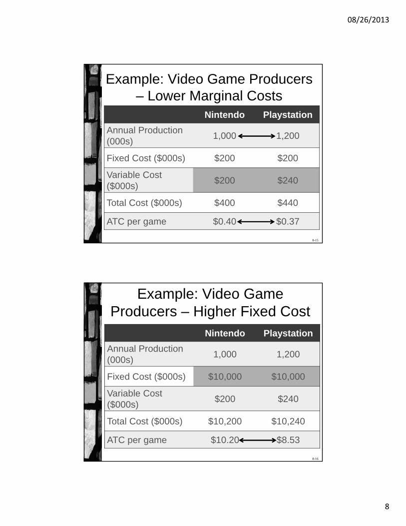
Example: Video Game Producers – Lower Marginal Costs



1,000 1,200

Fixed Cost ($000s) $200 $200


$200 $240

Total Cost ($000s) $400 $440


8-16

Example: Video Game Producers – Higher Fixed Cost



1,000 1,200

Fixed Cost ($000s) $10,000 $10,000


$200 $240

Total Cost ($000s) $10,200 $10,240


08/26/2013

9

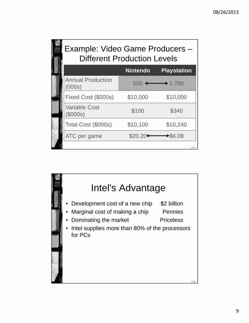
8-17

Example: Video Game Producers –Different Production Levels



500 1,700

Fixed Cost ($000s) $10,000 $10,000


$100 $340

Total Cost ($000s) $10,100 $10,240


8-18

Intel's Advantage

• Development cost of a new chip $2 billion

• Marginal cost of making a chip Pennies

• Dominating the market Priceless

• Intel supplies more than 80% of the processors for PCs

08/26/2013

10

8-19

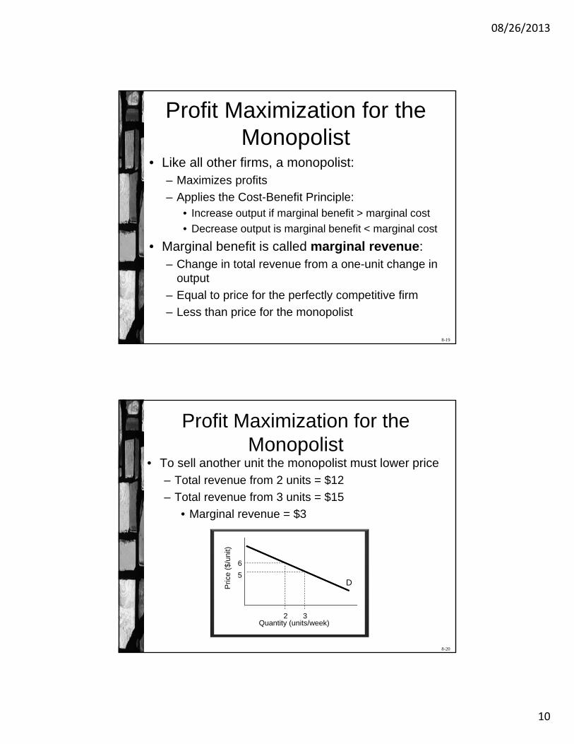
Profit Maximization for the Monopolist

• Like all other firms, a monopolist:– Maximizes profits

– Applies the Cost-Benefit Principle:• Increase output if marginal benefit > marginal cost

• Decrease output is marginal benefit < marginal cost

• Marginal benefit is called marginal revenue:– Change in total revenue from a one-unit change in

output

– Equal to price for the perfectly competitive firm

– Less than price for the monopolist

8-20

Pric

e ($

/uni

t)

Quantity (units/week)

Profit Maximization for the Monopolist

• To sell another unit the monopolist must lower price– Total revenue from 2 units = $12

– Total revenue from 3 units = $15

• Marginal revenue = $3

D

2

6

3

5

08/26/2013

11

8-21

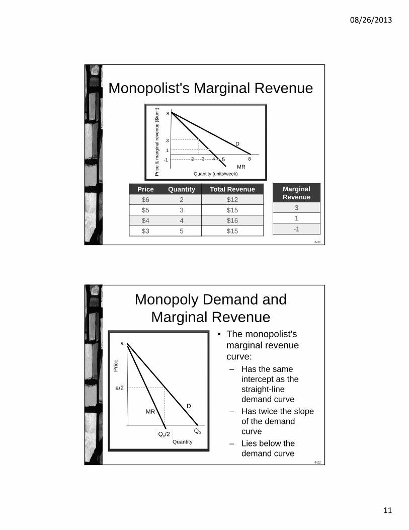
Monopolist's Marginal Revenue

Total Revenue

$12

$15

$16

$15

Price Quantity

$6 2

$5 3

$4 4

$3 5

Pric

e &

mar

gina

l rev

enue

($/

unit)

8

8

D


MR

32

3

1

4-1 5

Marginal Revenue

3

1

-1

8-22

Monopoly Demand and Marginal Revenue

• The monopolist's marginal revenue curve:– Has the same

intercept as the straight-line demand curve

– Has twice the slope of the demand curve

– Lies below the demand curve

Pri

ce

Quantity

a

D

Q0Q0/2

a/2

MR

08/26/2013

12

8-23

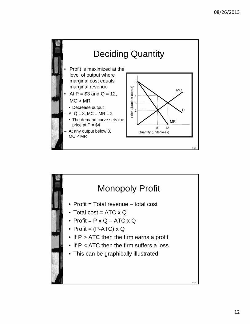
Deciding Quantity

• Profit is maximized at the level of output where marginal cost equals marginal revenue

• At P = $3 and Q = 12,

MC > MR• Decrease output

– At Q = 8, MC = MR = 2

• The demand curve sets the price at P = $4

– At any output below 8, MC < MR

Pric

e ($

/uni

t of

out

put)


3

MC

2

6

D

12

MR

4

8

8-24

Monopoly Profit

• Profit = Total revenue – total cost

• Total cost = ATC x Q

• Profit = P x Q – ATC x Q

• Profit = (P-ATC) x Q

• If P > ATC then the firm earns a profit

• If P < ATC then the firm suffers a loss

• This can be graphically illustrated

08/26/2013

13

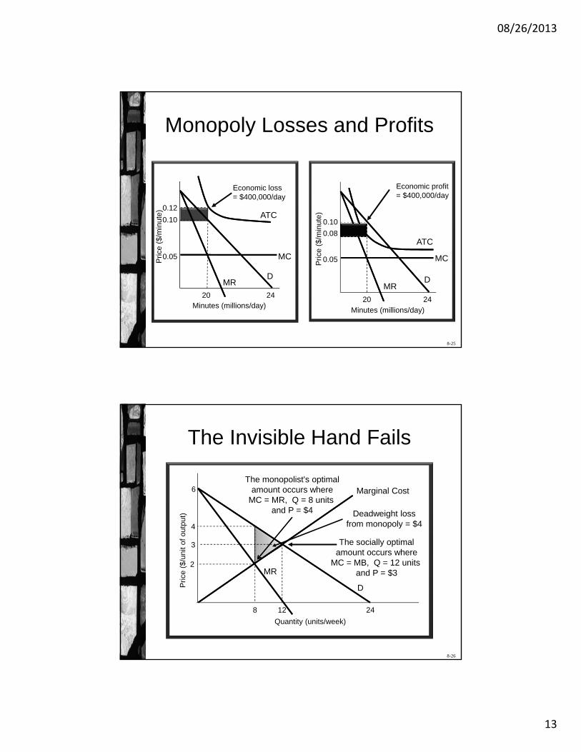
8-25

Monopoly Losses and ProfitsP

rice

($/m

inut

e)

Minutes (millions/day)20

0.12

0.10ATC

Economic loss= $400,000/day

D

0.05 MC

MR

24

Pric

e ($

/min

ute)

Minutes (millions/day)

2420

0.08

0.10

ATC

D

0.05 MC

MR

Economic profit= $400,000/day

8-26

The Invisible Hand Fails

Pric

e ($

/uni

t of

out

put)


The socially optimalamount occurs where

MC = MB, Q = 12 units and P = $3

The monopolist's optimalamount occurs where

MC = MR, Q = 8 units and P = $4

2MR

8

4

24

D

3

12

6 Marginal Cost

Deadweight loss from monopoly = $4

08/26/2013

14

8-27

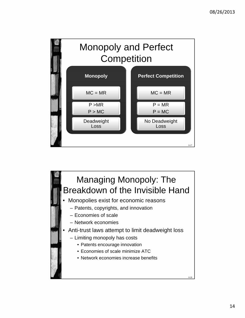
Monopoly and Perfect Competition

Monopoly

MC = MR

P >MR

P > MC

Deadweight Loss

Perfect Competition

MC = MR

P = MR

P = MC

No Deadweight Loss

8-28

Managing Monopoly: The Breakdown of the Invisible Hand• Monopolies exist for economic reasons

– Patents, copyrights, and innovation

– Economies of scale

– Network economies

• Anti-trust laws attempt to limit deadweight loss– Limiting monopoly has costs

• Patents encourage innovation

• Economies of scale minimize ATC

• Network economies increase benefits

08/26/2013

15

8-29

Price Discrimination

• Price discrimination means charging different buyers different prices for essentially the same good or service– Separate the groups

– No side trades among buyers

• Many forms of price discrimination– Hurdle method: discounts for identifiable groups

(e. g., students, AARP)

– Perfect discrimination: negotiate separate deals with each customer

8-30

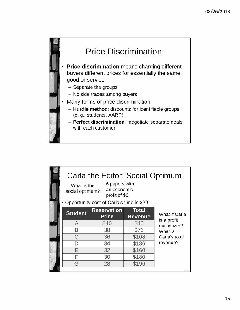
Carla the Editor: Social Optimum

• Opportunity cost of Carla's time is $29

What is the social optimum?

What if Carla is a profit maximizer? What is Carla's total revenue?

Student Reservation

Price A $40 B 38C 36D 34E 32F 30G 28

Total Revenue

$40 $76

$108 $136 $160 $180 $196

6 papers with an economic profit of $6

08/26/2013

16

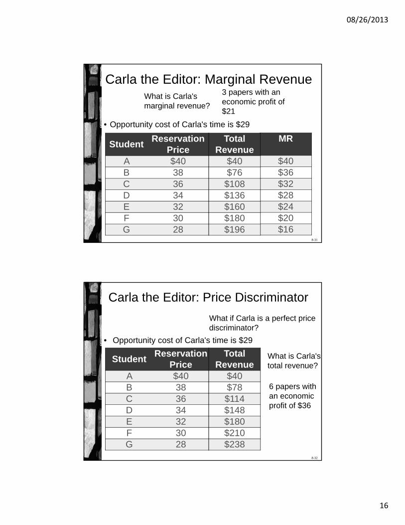
8-31

Carla the Editor: Marginal Revenue


What is Carla's marginal revenue?

Student Reservation

Price A $40 B 38C 36D 34E 32F 30G 28

MR

$40 $36 $32 $28 $24 $20 $16

Total Revenue

$40 $76

$108 $136 $160 $180 $196

3 papers with an economic profit of $21

8-32

Carla the Editor: Price Discriminator


What if Carla is a perfect price discriminator?

What is Carla's total revenue?

Student Reservation

Price A $40 B 38C 36D 34E 32F 30G 28

Total Revenue

$40 $78 $114 $148 $180 $210 $238

6 papers with an economicprofit of $36

08/26/2013

17

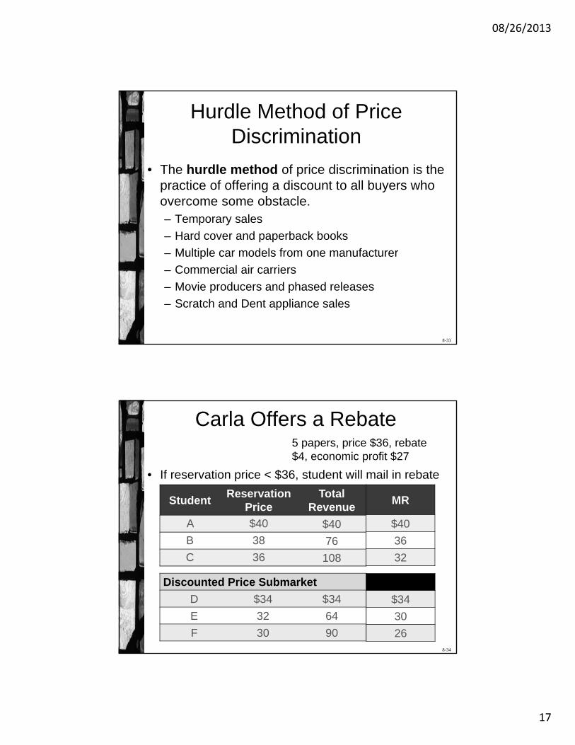
8-33

Hurdle Method of Price Discrimination

• The hurdle method of price discrimination is the practice of offering a discount to all buyers who overcome some obstacle.– Temporary sales

– Hard cover and paperback books

– Multiple car models from one manufacturer

– Commercial air carriers

– Movie producers and phased releases

– Scratch and Dent appliance sales

8-34

Carla Offers a Rebate

• If reservation price < $36, student will mail in rebate

StudentReservation

PriceTotal

Revenue

A $40 $40

B 38 76

C 36 108

Discounted Price Submarket

D $34 $34

E 32 64

F 30 90

MR

$40

36

32

$34

30

26

5 papers, price $36, rebate $4, economic profit $27

08/26/2013

18

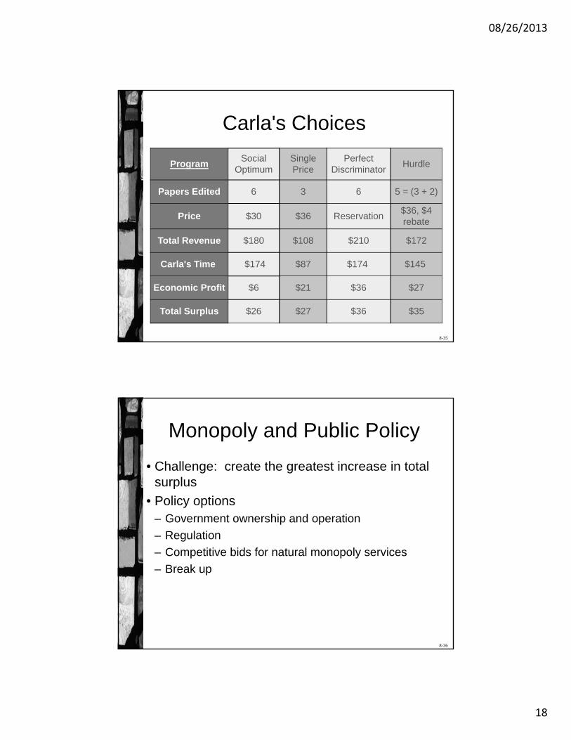
8-35

Carla's Choices

Program Social

Optimum

Papers Edited 6

Price $30

Total Revenue $180

Carla's Time $174

Economic Profit $6

Total Surplus $26

Hurdle

5 = (3 + 2)

$36, $4 rebate

$172

$145

$27

$35

Perfect Discriminator

6

Reservation

$210

$174

$36

$36

Single Price

3

$36

$108

$87

$21

$27

8-36

Monopoly and Public Policy

• Challenge: create the greatest increase in total surplus

• Policy options– Government ownership and operation

– Regulation

– Competitive bids for natural monopoly services

– Break up

08/26/2013

19

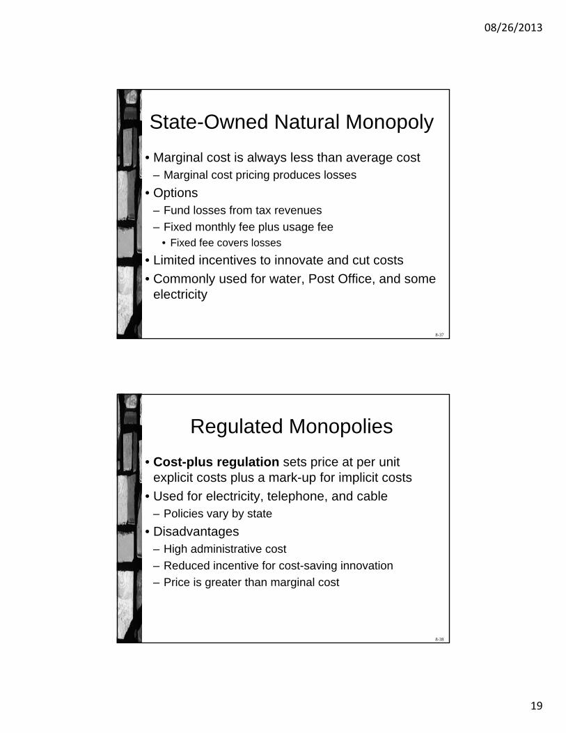
8-37

State-Owned Natural Monopoly

• Marginal cost is always less than average cost– Marginal cost pricing produces losses

• Options– Fund losses from tax revenues

– Fixed monthly fee plus usage fee • Fixed fee covers losses

• Limited incentives to innovate and cut costs

• Commonly used for water, Post Office, and some electricity

8-38

Regulated Monopolies

• Cost-plus regulation sets price at per unit explicit costs plus a mark-up for implicit costs

• Used for electricity, telephone, and cable– Policies vary by state

• Disadvantages– High administrative cost

– Reduced incentive for cost-saving innovation

– Price is greater than marginal cost

08/26/2013

20

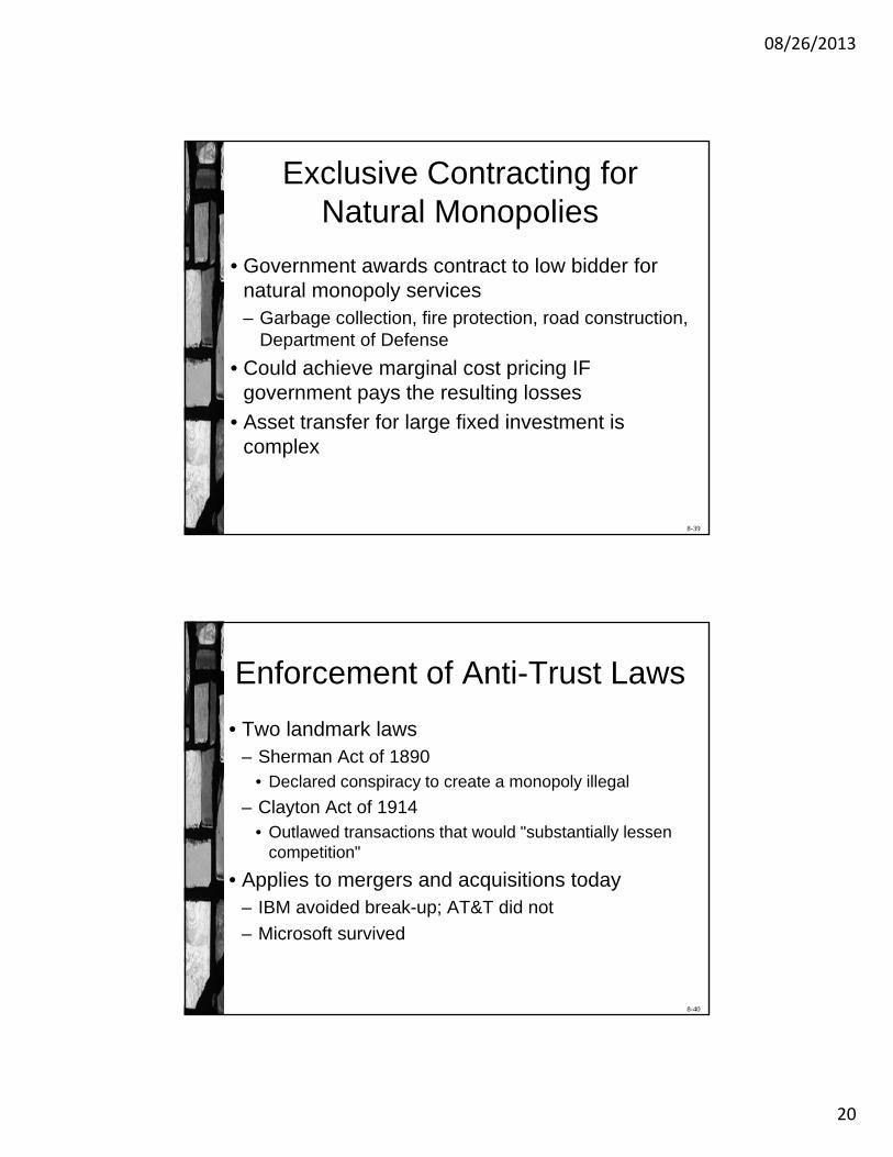
8-39

Exclusive Contracting for Natural Monopolies

• Government awards contract to low bidder for natural monopoly services– Garbage collection, fire protection, road construction,

Department of Defense

• Could achieve marginal cost pricing IF government pays the resulting losses

• Asset transfer for large fixed investment is complex

8-40

Enforcement of Anti-Trust Laws

• Two landmark laws– Sherman Act of 1890

• Declared conspiracy to create a monopoly illegal

– Clayton Act of 1914• Outlawed transactions that would "substantially lessen

competition"

• Applies to mergers and acquisitions today– IBM avoided break-up; AT&T did not

– Microsoft survived

08/26/2013

21

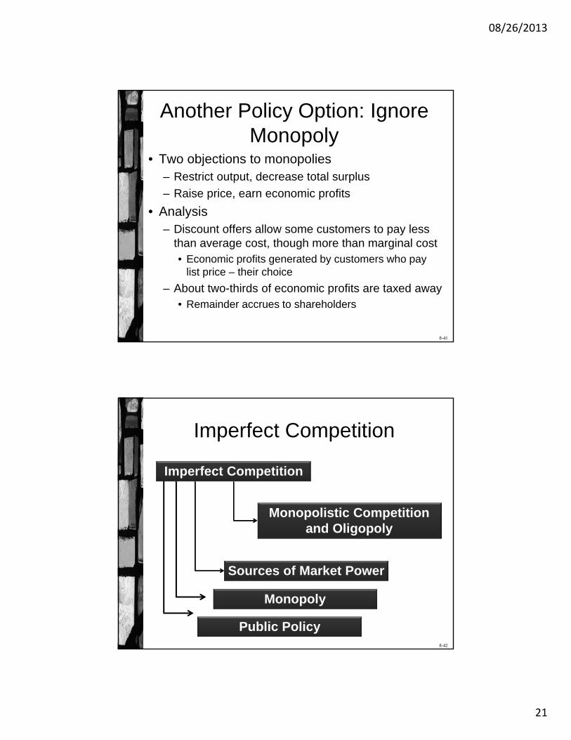
8-41

Another Policy Option: Ignore Monopoly

• Two objections to monopolies– Restrict output, decrease total surplus

– Raise price, earn economic profits

• Analysis– Discount offers allow some customers to pay less

than average cost, though more than marginal cost• Economic profits generated by customers who pay

list price – their choice

– About two-thirds of economic profits are taxed away• Remainder accrues to shareholders

8-42



Monopolistic Competition and Oligopoly

Sources of Market Power

Monopoly

Public Policy

08/26/2013

22

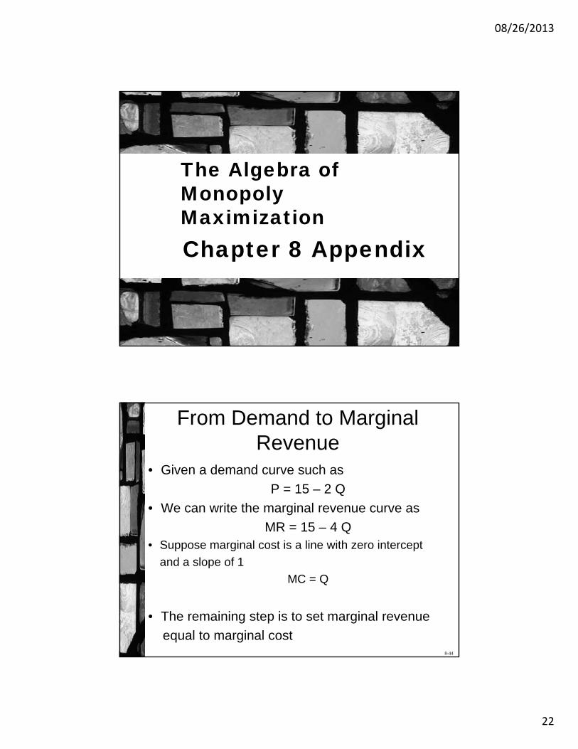
Chapter 8 Appendix

The Algebra of Monopoly Maximization

8-44

From Demand to Marginal Revenue

• Given a demand curve such as

P = 15 – 2 Q

• We can write the marginal revenue curve as

MR = 15 – 4 Q• Suppose marginal cost is a line with zero intercept

and a slope of 1

MC = Q

• The remaining step is to set marginal revenue

equal to marginal cost

08/26/2013

23

8-45

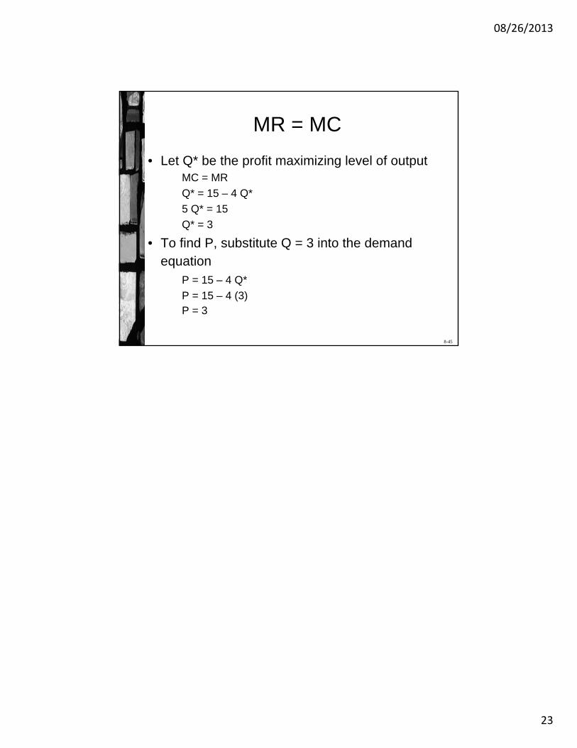
MR = MC

• Let Q* be the profit maximizing level of outputMC = MR

Q* = 15 – 4 Q*

5 Q* = 15

Q* = 3

• To find P, substitute Q = 3 into the demand equation

P = 15 – 4 Q*

P = 15 – 4 (3)P = 3

Education

Chap008 lecture