Embed Size (px)
Citation preview
Measuring the behavioral component of financial fluctuaction. An analysis based on the S&P 500.
SYstemic Risk TOmography:Signals, Measurements, Transmission Channels, and Policy Interventions
M. Caporin, University of Padova (Italy)L. Corazzini, University of Padova (Italy)M. Costola, Ca' Foscari University of Venice (Italy)
ASSET 2013– Bilbao (ES). November 8, 2013.
Intro Literature Review The rational agent The Behavioral agent The Model Empirical Analysis τ∗ and investor sentiment Conclusion
Measuring the behavioral componentof financial fluctuations:
An analysis based on the S&P500.
Massimiliano Caporin Luca Corazzini Michele Costola
Ca’ Foscari University of Venice
Asset 2013, Bilbao.
Intro Literature Review The rational agent The Behavioral agent The Model Empirical Analysis τ∗ and investor sentiment Conclusion
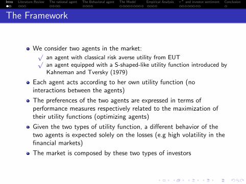
The Framework
We consider two agents in the market:√
an agent with classical risk averse utility from EUT√an agent equipped with a S-shaped-like utility function introduced byKahneman and Tversky (1979)
Each agent acts according to her own utility function (nointeractions between the agents)
The preferences of the two agents are expressed in terms ofperformance measures respectively related to the maximization oftheir utility functions (optimizing agents)
Given the two types of utility function, a different behavior of thetwo agents is expected solely on the losses (e.g high volatility in thefinancial markets)
The market is composed by these two types of investors
Intro Literature Review The rational agent The Behavioral agent The Model Empirical Analysis τ∗ and investor sentiment Conclusion
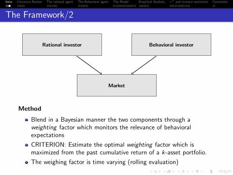
The Framework/2
Market
Rational investor Behavioral investor
Method
Blend in a Bayesian manner the two components through aweighting factor which monitors the relevance of behavioralexpectations
CRITERION: Estimate the optimal weighting factor which ismaximized from the past cumulative return of a k-asset portfolio.
The weighing factor is time varying (rolling evaluation)
Intro Literature Review The rational agent The Behavioral agent The Model Empirical Analysis τ∗ and investor sentiment Conclusion
Behavioral Finance
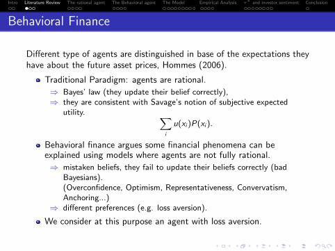
Different type of agents are distinguished in base of the expectations theyhave about the future asset prices, Hommes (2006).
Traditional Paradigm: agents are rational.
⇒ Bayes’ law (they update their belief correctly),⇒ they are consistent with Savage’s notion of subjective expected
utility. ∑i
u(xi )P(xi ).
Behavioral finance argues some financial phenomena can beexplained using models where agents are not fully rational.
⇒ mistaken beliefs, they fail to update their beliefs correctly (badBayesians).(Overconfidence, Optimism, Representativeness, Convervatism,Anchoring...)
⇒ different preferences (e.g. loss aversion).
We consider at this purpose an agent with loss aversion.
Intro Literature Review The rational agent The Behavioral agent The Model Empirical Analysis τ∗ and investor sentiment Conclusion
Loss Aversion at the level of the individual stocks
Barberis et al. (2001) shows that an economy where investors are lossaverse over the fluctuations of individual stocks reflects more empiricalphenomena w.r.t an economy where investors are loss averse over thefluctuations of their stock portfolio.
Firm level returns have a high mean, are excessively volatile, and arepredictable in the time series using lagged variables,
the premium to value stocks and to stocks with poor prior returns,
cross-sectional facts: the discount rate is function of the pastperformance returns.
Intro Literature Review The rational agent The Behavioral agent The Model Empirical Analysis τ∗ and investor sentiment Conclusion
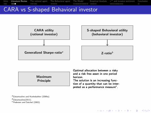
CARA vs S-shaped Behavioral investor
CARA utility(rational investor)
S-shaped Behavioral utility(behavioral investor)
Generalized Sharpe-ratioa Z-ratiob
MaximumPrinciple
Optimal allocation between a riskyand a risk free asset in one periodhorizon.The solution is an increasing func-tion of a quantity that can be inter-preted as a performance measurec .
Optimal allocation between a riskyand a risk free asset in one periodhorizon.The solution is an increasing func-tion of a quantity that can be inter-preted as a performance measurec .
aZakamouline and Koekebakker (2009a).bZakamouline(2011).cPedersen and Satchel (2002).
Intro Literature Review The rational agent The Behavioral agent The Model Empirical Analysis τ∗ and investor sentiment Conclusion
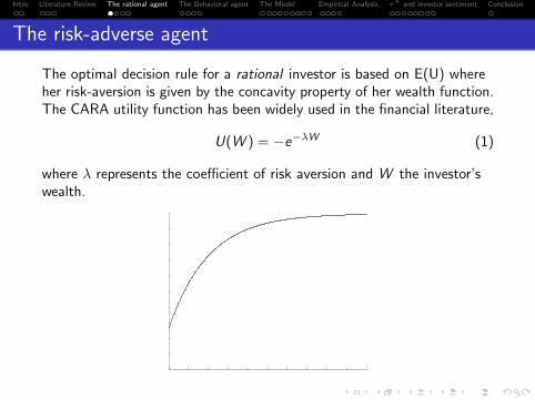
The risk-adverse agent
The optimal decision rule for a rational investor is based on E(U) whereher risk-aversion is given by the concavity property of her wealth function.The CARA utility function has been widely used in the financial literature,
U(W ) = −e−λW (1)
where λ represents the coefficient of risk aversion and W the investor’swealth.
Intro Literature Review The rational agent The Behavioral agent The Model Empirical Analysis τ∗ and investor sentiment Conclusion
The Sharpe ratio
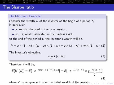
The Maximum Principle
Consider the wealth w of the investor at the begin of a period t0.In particular,
a, wealth allocated in the risky asset x ,
w − a, wealth allocated in the riskless asset.
At the end of the period t1 the investor’s wealth will be,
w = a× (1 + x) + (w − a)× (1 + rf ) = a× (x − rf ) + w × (1 + rf ) (2)
The investor’s objective,maxa
E [U(w)]. (3)
Therefore it will be,
E [U∗(w)] = E [−e−λ[a(x−rf )+w(1+rf )]] = E [−e−λ[a(x−rf )] × e−λw(1+rf )︸ ︷︷ ︸q
]
(4)where a∗ is independent from the initial wealth of the investor.
Intro Literature Review The rational agent The Behavioral agent The Model Empirical Analysis τ∗ and investor sentiment Conclusion
The Sharpe ratio
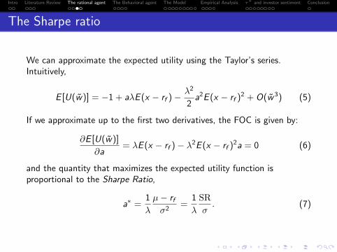
We can approximate the expected utility using the Taylor’s series.Intuitively,
E [U(w)] = −1 + aλE (x − rf )− λ2
2a2E (x − rf )2 + O(w3) (5)
If we approximate up to the first two derivatives, the FOC is given by:
∂E [U(w)]
∂a= λE (x − rf )− λ2E (x − rf )2a = 0 (6)
and the quantity that maximizes the expected utility function isproportional to the Sharpe Ratio,
a∗ =1
λ
µ− rfσ2
=1
λ
SR
σ. (7)
Intro Literature Review The rational agent The Behavioral agent The Model Empirical Analysis τ∗ and investor sentiment Conclusion
Generalized Sharpe Ratio
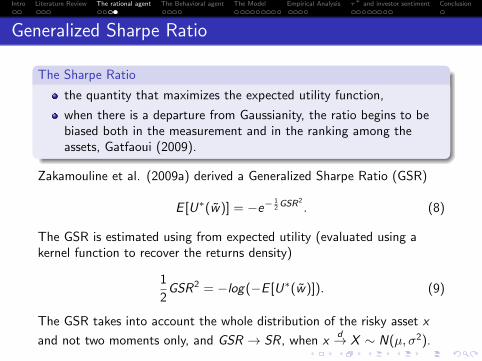
The Sharpe Ratio
the quantity that maximizes the expected utility function,
when there is a departure from Gaussianity, the ratio begins to bebiased both in the measurement and in the ranking among theassets, Gatfaoui (2009).
Zakamouline et al. (2009a) derived a Generalized Sharpe Ratio (GSR)
E [U∗(w)] = −e− 12GSR
2
. (8)
The GSR is estimated using from expected utility (evaluated using akernel function to recover the returns density)
1
2GSR2 = −log(−E [U∗(w)]). (9)
The GSR takes into account the whole distribution of the risky asset x
and not two moments only, and GSR → SR, when xd→ X ∼ N(µ, σ2).
Intro Literature Review The rational agent The Behavioral agent The Model Empirical Analysis τ∗ and investor sentiment Conclusion
The S-shaped Utility Function
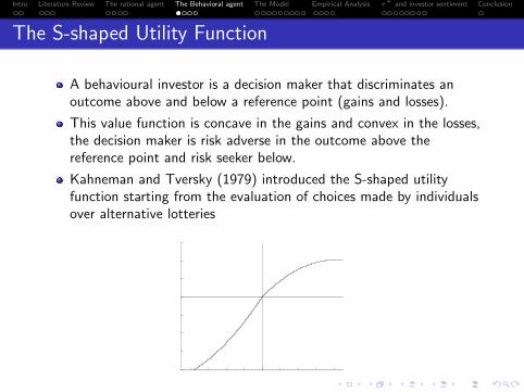
A behavioural investor is a decision maker that discriminates anoutcome above and below a reference point (gains and losses).
This value function is concave in the gains and convex in the losses,the decision maker is risk adverse in the outcome above thereference point and risk seeker below.
Kahneman and Tversky (1979) introduced the S-shaped utilityfunction starting from the evaluation of choices made by individualsover alternative lotteries
Intro Literature Review The rational agent The Behavioral agent The Model Empirical Analysis τ∗ and investor sentiment Conclusion
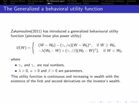
The Generalized a behavioral utility function
Zakamouline(2011) has introduced a generalized behavioural utilityfunction (piecewise linear plus power utility)
U(W ) =
{(W −W0)− (γ+/α)(W −W0)α, if W ≥W0,
−λ(W0 −W ) + (γ−/β)(W0 −W )β), if W <W0,
where
γ+ and γ− are real numbers,
λ > 0, α > 0 and β > 0 are parameters.
This utility function is continuous and increasing in wealth with theexistence of the first and second derivatives on the investor’s wealth.
Intro Literature Review The rational agent The Behavioral agent The Model Empirical Analysis τ∗ and investor sentiment Conclusion
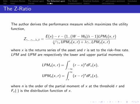
The Z-Ratio
The author derives the performance measure which maximizes the utilityfunction,
Zγ−,γ+,λ,β =E (x)− r − (1−(W −W0)λ− 1)LPM1(x , r)
β√γ+UPMβ(x , r) + λγ−LPMβ(x , r)
where x is the returns series of the asset and r is set to the risk–free rate.LPM and UPM are respectively the lower and upper partial moments,
LPMn(x , r) =
∫ r
−∞(r − x)ndFx(x),
UPMn(x , r) =
∫ ∞r
(x − r)ndFx(x),
where n is the order of the partial moment of x at the threshold r andFx(·) is the distribution function of x .
Intro Literature Review The rational agent The Behavioral agent The Model Empirical Analysis τ∗ and investor sentiment Conclusion
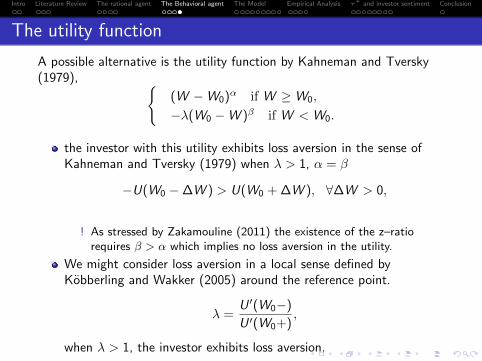
The utility function
A possible alternative is the utility function by Kahneman and Tversky(1979), {
(W −W0)α if W ≥W0,
−λ(W0 −W )β if W <W0.
the investor with this utility exhibits loss aversion in the sense ofKahneman and Tversky (1979) when λ > 1, α = β
−U(W0 −∆W ) > U(W0 + ∆W ), ∀∆W > 0,
! As stressed by Zakamouline (2011) the existence of the z–ratiorequires β > α which implies no loss aversion in the utility.
We might consider loss aversion in a local sense defined byKobberling and Wakker (2005) around the reference point.
λ =U ′(W0−)
U ′(W0+),
when λ > 1, the investor exhibits loss aversion.
Intro Literature Review The rational agent The Behavioral agent The Model Empirical Analysis τ∗ and investor sentiment Conclusion
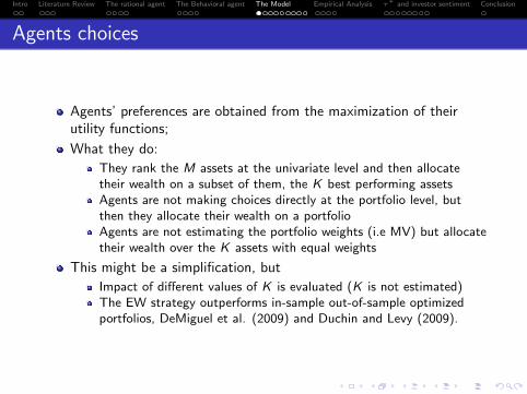
Agents choices
Agents’ preferences are obtained from the maximization of theirutility functions;
What they do:
They rank the M assets at the univariate level and then allocatetheir wealth on a subset of them, the K best performing assetsAgents are not making choices directly at the portfolio level, butthen they allocate their wealth on a portfolioAgents are not estimating the portfolio weights (i.e MV) but allocatetheir wealth over the K assets with equal weights
This might be a simplification, but
Impact of different values of K is evaluated (K is not estimated)The EW strategy outperforms in-sample out-of-sample optimizedportfolios, DeMiguel et al. (2009) and Duchin and Levy (2009).
Intro Literature Review The rational agent The Behavioral agent The Model Empirical Analysis τ∗ and investor sentiment Conclusion
Agents choices and the market
Our purpose is to focus on the entire market, as influenced by thechoices made by the two types of agents
We take thus the market point of view, or the view of an imaginaryoptimizing agent willing to take investment decisions accounting forboth rational and behavioral points of view (with the sameallocation scheme adopted by rational/behavioral)
The question is: how much should I have trusted behavioral/rationalviews to allocate my portfolio in the optimal way?
We thus introduce a framework where a parameter allows us tomonitor the relevance of behavioral choices (it will not be a relativeweight of behavioral agents nor the relative weight of behavioralrankings over rational rankings)
At the market level we act starting from a rational point of view, insuch a way the impact of behavioral choices might be null in alimiting case
Intro Literature Review The rational agent The Behavioral agent The Model Empirical Analysis τ∗ and investor sentiment Conclusion
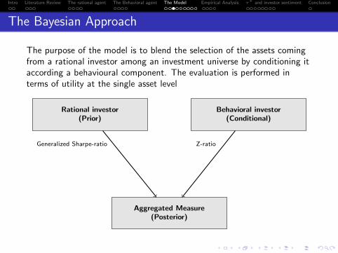
The Bayesian Approach
The purpose of the model is to blend the selection of the assets comingfrom a rational investor among an investment universe by conditioning itaccording a behavioural component. The evaluation is performed interms of utility at the single asset level
Aggregated Measure(Posterior)
Rational investor(Prior)
Behavioral investor(Conditional)
Generalized Sharpe-ratio Z-ratio
Intro Literature Review The rational agent The Behavioral agent The Model Empirical Analysis τ∗ and investor sentiment Conclusion
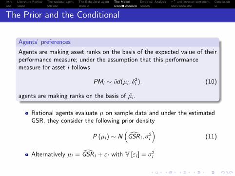
The Prior and the Conditional
Agents’ preferences
Agents are making asset ranks on the basis of the expected value of theirperformance measure; under the assumption that this performancemeasure for asset i follows
PMi ∼ iid(µi , δ2i ). (10)
agents are making ranks on the basis of µi .
Rational agents evaluate µ on sample data and under the estimatedGSR, they consider the following prior density
P (µi ) ∼ N(GSR i , σ
2i
)(11)
Alternatively µi = GSR i + εi with V [εi ] = σ2i
Intro Literature Review The rational agent The Behavioral agent The Model Empirical Analysis τ∗ and investor sentiment Conclusion
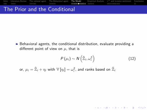
The Prior and the Conditional
Behavioral agents, the conditional distribution, evaluate providing adifferent point of view on µ, that is
P (µi ) ∼ N(Zi , ω
2i
)(12)
or, µi = Zi + ηi with V [ηi ] = ω2i , and ranks based on Zi
Intro Literature Review The rational agent The Behavioral agent The Model Empirical Analysis τ∗ and investor sentiment Conclusion
The Prior and the Conditional
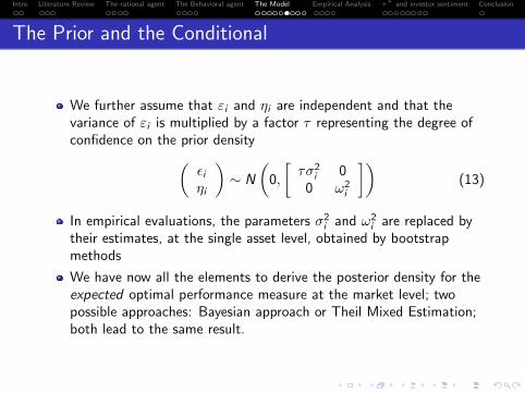
We further assume that εi and ηi are independent and that thevariance of εi is multiplied by a factor τ representing the degree ofconfidence on the prior density(
εiηi
)∼ N
(0,
[τσ2
i 00 ω2
i
])(13)
In empirical evaluations, the parameters σ2i and ω2
i are replaced bytheir estimates, at the single asset level, obtained by bootstrapmethods
We have now all the elements to derive the posterior density for theexpected optimal performance measure at the market level; twopossible approaches: Bayesian approach or Theil Mixed Estimation;both lead to the same result.
Intro Literature Review The rational agent The Behavioral agent The Model Empirical Analysis τ∗ and investor sentiment Conclusion
The Posterior
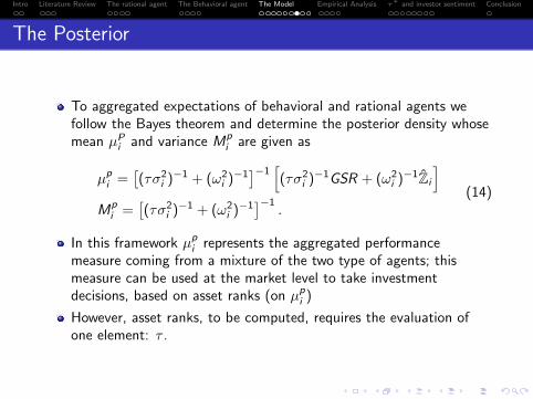
To aggregated expectations of behavioral and rational agents wefollow the Bayes theorem and determine the posterior density whosemean µP
i and variance Mpi are given as
µpi =
[(τσ2
i )−1 + (ω2i )−1
]−1 [(τσ2
i )−1GSR + (ω2i )−1Zi
]Mp
i =[(τσ2
i )−1 + (ω2i )−1
]−1.
(14)
In this framework µpi represents the aggregated performance
measure coming from a mixture of the two type of agents; thismeasure can be used at the market level to take investmentdecisions, based on asset ranks (on µp
i )
However, asset ranks, to be computed, requires the evaluation ofone element: τ .
Intro Literature Review The rational agent The Behavioral agent The Model Empirical Analysis τ∗ and investor sentiment Conclusion
The estimation of τ ∗
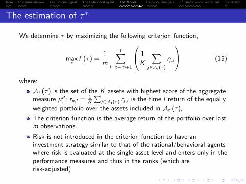
We determine τ by maximizing the following criterion function,
maxτ
f (τ) =1
m
t∑l=t−m+1
1
K
∑j∈At(τ)
rj,l
(15)
where:
At (τ) is the set of the K assets with highest score of the aggregatemeasure µp
i ; rp,l = 1K
∑j∈At(τ)
rj,l is the time l return of the equally
weighted portfolio over the assets included in At (τ),
The criterion function is the average return of the portfolio over lastm observations
Risk is not introduced in the criterion function to have aninvestment strategy similar to that of the rational/behavioral agentswhere risk is evaluated at the single asset level and enters only in theperformance measures and thus in the ranks (which arerisk-adjusted)
Intro Literature Review The rational agent The Behavioral agent The Model Empirical Analysis τ∗ and investor sentiment Conclusion
The interpretation of τ ∗
The purpose is to estimate τ∗ for the aggregated measure µpi
according the criterion function which optimizes the cumulativereturn of K assets.
That is, we want to check for which value of τ∗ we would haveobtained the optimal cumulative return of a portfolio with K assetsfor a given period.
In fact, a higher value of τ∗ would imply that the investor shouldhave correct her action towards a behavioral direction.Conversely, a low value of τ∗ would imply that the investor shouldhave remained on her prior rational ranks.
Therefore, with the criterion function we are detecting the relativeimportance of the behavioral choices over the rational ones.
τ∗ is in some sense related to impact of behavioral choices on themarket fluctuations in a given moment.
Intro Literature Review The rational agent The Behavioral agent The Model Empirical Analysis τ∗ and investor sentiment Conclusion
The dataset and the Model Settings
We consider the constituents at a given time t of the S&P500 fromJanuary 1962 to February 2012 at a monthly frequency (sourceCRSP/COMPUSTAT)
The model has been applied on rolling windows of 60 monthlyreturns (shorter evaluation windows provide more noisy and volatileevaluations of the performance measures)
Thus, we selected from the constituents of the S&P500 at a given tsolely the assets with at least 60 observations.
The variance of the measures is obtained using a block bootstrapprocedure (dimension of blocks 4).
We initially select K = 100 to reflect the dimension of a stock indexas S&P100 (which is equally weighted).
Intro Literature Review The rational agent The Behavioral agent The Model Empirical Analysis τ∗ and investor sentiment Conclusion
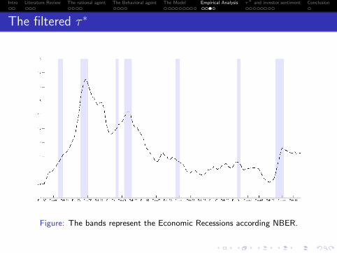
The filtered τ ∗
To smooth the optimized τ∗ we filtered it with a local level model{τ∗t = µt + εt , εt ∼ NID(0, σ2
ε )
µt+1 = µt + ξt , ξt ∼ NID(0, σ2ξ)
(16)
µt is the unobserved level for t = 1, . . . , n,
εt is the observation disturbance and ξt is the level disturbance atime t.
For the investor equipped with an utility function similar to Kahnemanand Tversky (1979), we estimated εt ∼ NID(0, .4547) andξt ∼ NID(0, .001678).
Intro Literature Review The rational agent The Behavioral agent The Model Empirical Analysis τ∗ and investor sentiment Conclusion
The filtered τ ∗
Figure: The bands represent the Economic Recessions according NBER.
Intro Literature Review The rational agent The Behavioral agent The Model Empirical Analysis τ∗ and investor sentiment Conclusion
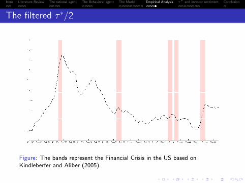
The filtered τ ∗/2
Figure: The bands represent the Financial Crisis in the US based onKindleberfer and Aliber (2005).
Intro Literature Review The rational agent The Behavioral agent The Model Empirical Analysis τ∗ and investor sentiment Conclusion
τ ∗ and investor sentiment
Our estimate of the confidence on rational priors can be linked tothe literature of market sentiment indices
Market sentiment indices monitor the general view on the market,i.e. bullish/bearish
Moreover, sentiment indices can have a behavioralcomponent/interpretation
Linking the τ∗ to sentiment indices allows verifying how muchbehavioral views are related to the evolution of market sentiment,with an expected positive relation
Several indices of market sentiment: VIX (fear index), volume,liquidity, and other (Baker and Wurgler, 2007)
Intro Literature Review The rational agent The Behavioral agent The Model Empirical Analysis τ∗ and investor sentiment Conclusion
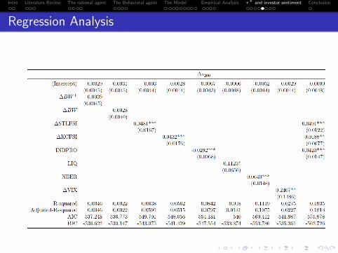
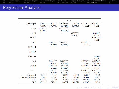
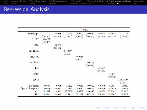
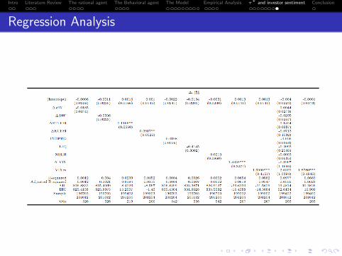
Market sentiments and Economic indicators
Our factor τ ,⇒ can be interpreted as a quantity associated to agent’s overallbehaviour in period of market stress.⇒ We can relate its evolution to other indicators that monitor the levelof financial stress,
FSIs capture the key features of market stress: i.e increasesuncertainty about fundamental value of asset, increased uncertaintyabout behavior of other investors, increased information asymmetry,
Sentiment indicator (Baker and Wurgler, 2007),
NBER recessions (dummy),
Liquidity indicator (Paster and Stambaugh, 2001),
Industrial Production.
Intro Literature Review The rational agent The Behavioral agent The Model Empirical Analysis τ∗ and investor sentiment Conclusion
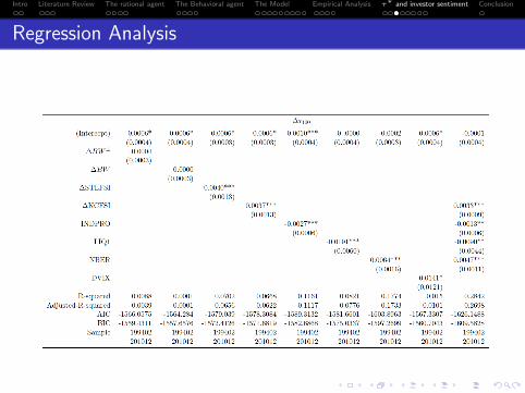
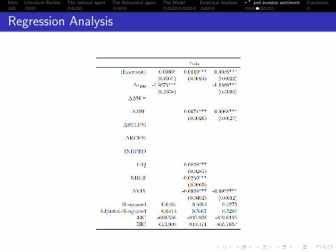
Regression Analysis
Intro Literature Review The rational agent The Behavioral agent The Model Empirical Analysis τ∗ and investor sentiment Conclusion
Regression Analysis
Intro Literature Review The rational agent The Behavioral agent The Model Empirical Analysis τ∗ and investor sentiment Conclusion
Regression Analysis
Intro Literature Review The rational agent The Behavioral agent The Model Empirical Analysis τ∗ and investor sentiment Conclusion
Regression Analysis
Intro Literature Review The rational agent The Behavioral agent The Model Empirical Analysis τ∗ and investor sentiment Conclusion
Regression Analysis
Intro Literature Review The rational agent The Behavioral agent The Model Empirical Analysis τ∗ and investor sentiment Conclusion
Regression Analysis
Intro Literature Review The rational agent The Behavioral agent The Model Empirical Analysis τ∗ and investor sentiment Conclusion
Conclusion
We estimated a time varying weighting factor on the S&P500according on the maximization on the cumulative returns.
We found some interesting similarities between the localmaxima/minima of the estimated factor and economic recessions(NBER) and financial crisis.
We found a relationship with the financial sentiment and othereconomic indicators when analysing the relation between ourestimated parameter and sentiment indices
We can consider our indicator as a possible endogenous marketsentiment index.
Robustness checks: analyses on the role of K and with an“opposite” utility function.
Use τ as a pricing factor at single-asset level or for macro-sector.

This project has received funding from the European Union’s Seventh Framework Programme for research, technological
development and demonstration under grant agreement n° 320270
www.syrtoproject.eu