Genuine Saving and Conspicuous Consumption · (2010), and Corazzini, Esposito, and Majorano (2012). See also Fliessbach et al. (2007) and Dohmen et al

Department of Economics School of Business, Economics and Law at University of Gothenburg Vasagatan 1, PO Box 640, SE 405 30 Göteborg, Sweden +46 31 786 0000, +46 31 786 1326 (fax) www.handels.gu.se [email protected]

WORKING PAPERS IN ECONOMICS

No 605

Genuine Saving and Conspicuous Consumption

Thomas Aronsson and Olof Johansson-Stenman

November 2014

ISSN 1403-2473 (print) ISSN 1403-2465 (online)

1

Genuine Saving and Conspicuous Consumption**

Thomas Aronsson* and Olof Johansson-Stenman+

November 2014

Abstract

Much evidence suggests that people are concerned with their relative consumption, i.e., their

consumption in relation to the consumption of others. Yet, the social costs of conspicuous

consumption have so far played little (or no) role in savings-based indicators of sustainable

development. The present paper examines the implications of such behavior for measures of

sustainable development by deriving analogues to genuine saving when people are concerned

with their relative consumption. Unless the resource allocation is a social optimum, an

indicator of positional externalities must be added to genuine saving to arrive at the proper

measure of intertemporal welfare change. A numerical example based on U.S. and Swedish

data suggests that conventional measures of genuine saving (which do not reflect conspicuous

consumption) are likely to largely overestimate this welfare change. We also show how

relative consumption concerns affect the way public investment ought to be reflected in

genuine saving.

JEL classification: D03, D60, D62, E21, H21, I31, Q56.

Keywords: Welfare change, investment, saving, relative consumption. ** The authors would like to thank Sofia Lundberg and Karl-Gustaf Löfgren for helpful comments and

suggestions, and Catia Cialani for collecting and organizing data. Research grants from the Swedish Research

Council (ref 421-2010-1420) are gratefully acknowledged. *Address: Department of Economics, Umeå School of Business and Economics, Umeå University, SE – 901 87

Umeå, Sweden. E-mail: [email protected] + Address: Department of Economics, School of Business, Economics and Law, University of Gothenburg, SE –

405 30 Gothenburg, Sweden. E-mail: [email protected]

2

1. Introduction

The concept of genuine saving has gained much attention in literature on welfare

measurement in dynamic economies. Genuine saving is an indicator of comprehensive net

investment in the sense of summarizing the value of all capital formation undertaken by

society over a time period. Earlier research shows that the genuine saving constitutes an exact

measure of welfare change over a short time interval if the resource allocation is first best.1

Furthermore, in the aftermath of the World Commission on Environment and Development,

genuine saving has also become an indicator of sustainable development. The World

Commission defines the development to be sustainable if it meets “the needs of the present

without compromising the ability of future generations to meet their own needs” (Our

Common Future, 1987, page 54). One possible interpretation (discussed by, e.g., Arrow et al.,

2003) is that sustainable development requires welfare to be non-declining, meaning that

genuine saving becomes an exact indicator of sustainable development over a short time

interval. Another is that the instantaneous utility must not exceed its maximum sustainable

level, on the basis of which Pezzey (2004) shows that non-positive genuine saving constitutes

an indicator of unsustainable development (although positive genuine saving does not

necessarily imply that development is sustainable). In either case, genuine saving gives

information of clear practical relevance for economic welfare.2

Yet, the literature dealing with genuine saving has so far focused on traditional

neoclassical textbook models, where people derive utility solely from their own absolute

consumption of goods and services (broadly defined). As such, it neglects the possibility

discussed in the behavioral economics literature that people also enjoy consuming more, and

dislike consuming less than others – an idea that appeared rather obvious to many leading

economists of the past such as Adam Smith, John Stuart Mill, Karl Marx, Alfred Marshall,

1 The seminal contributions are Pearce and Atkinson (1993) and Hamilton (1994, 1996). See also Hamilton

(2010) for a recent overview of the literature and van der Ploeg (2010) for a political economy analysis of

genuine saving. Some other extensions beyond the standard model are found in Aronsson, Cialani, and Löfgren

(2012) and Li and Löfgren (2012). The former derives a second-best analogue to genuine saving in a

representative agent model with distortionary taxes and public debt, and the latter addresses genuine saving

when growth is stochastic. See also the interesting, recent empirical application by Greasley et al. (2014), who

test the welfare significance of genuine saving based on historical data from Britain. 2 This is further emphasized by the attention paid to genuine saving by the World Bank, which regularly

publishes estimates of genuine saving for a large number of countries.

3

Thorstein Veblen and Arthur Pigou, before it became unfashionable in the beginning of the

20th century.

The purpose of the present paper is to examine how relative consumption concerns,

through a preference for “keeping-up-with-the-Joneses,” affect the principles for measuring

welfare change. It will then present a correspondingly adjusted measure of genuine saving.

Arguably, such a study is relevant for several reasons. First, there is now a large body of

empirical evidence showing that people are concerned with their relative consumption, i.e.,

their consumption compared with that of referent others (and not just their absolute

consumption as in standard economic models).3 Several studies find that increased relative

consumption has a strong effect on individual well-being: questionnaire-experimental

research often concludes that 30-50 percent of an individual’s utility gain from increased

consumption may actually be due to increased relative consumption (e.g., Alpizar et al., 2005;

Solnick and Hemenway, 2005; Carlsson et al., 2007). Similarly, happiness-based studies

typically find that a large (or even dominating) share of consumption-induced well-being in

industrialized countries is due to relative effects (e.g., Luttmer, 2005; Easterlin, 2001;

Easterlin et al., 2010). In turn, this may distort the incentives underlying capital formation.

Second, based on the estimates referred to above, wasteful conspicuous consumption is likely

to result in significant welfare costs, which – if not properly internalized – change the

principles for calculating welfare change-equivalent measures of saving. Indeed, we show that

the more positional people are on average, the more conventional models of genuine saving

(where people are assumed to have standard utility functions) will overestimate the true

welfare change. Third, recent literature shows that optimal policy rules for public expenditure

are modified in response to relative consumption concerns,4 suggesting that such concerns

may also affect the value of public investment in the context of genuine saving. This will be

further discussed below.

3 See, e.g., Easterlin (2001), Johansson-Stenman et al. (2002), Blanchflower and Oswald (2004), Ferrer-i-

Carbonell (2005), Luttmer (2005), Solnick and Hemenway (2005), Carlsson et al. (2007), Clark and Senik

(2010), and Corazzini, Esposito, and Majorano (2012). See also Fliessbach et al. (2007) and Dohmen et al.

(2011) for evidence based on brain science and Rayo and Becker (2007) for an evolutionary approach. 4 See Ng (1987), Brekke and Howarth (2002), Aronsson and Johansson-Stenman (2008, forthcoming), and

Wendner and Goulder (2008), who analyze different aspects of public good provision in economies where

people are concerned with their relative consumption.

4

We develop a dynamic general equilibrium model where each consumer derives utility

from his/her own consumption and use of leisure, respectively, and from his/her relative

consumption compared with a reference consumption level (reflecting other people’s

consumption). In the benchmark model, the relative consumption comparisons are of the

keeping-up-with-the-Joneses type, meaning that each individual compares his/her current

consumption with the current consumption of referent others, which is the case that best

corresponds to the empirical evidence discussed above. However, we will also – although

briefly – touch upon catching-up-with-the-Joneses comparisons, where the reference measure

refers to other people’s past consumption, and argue that the associated externalities affect the

welfare change measure in the same general way as the externalities following from keeping-

up-with-the-Joneses types of comparisons.

Our main contribution is that we show how positional concerns influence the way welfare-

change equivalent savings ought to be measured. We distinguish between a social optimum

where all externalities are internalized, and unregulated market economies without externality

correction. We also distinguish between first-best and second-best social optima by extending

the benchmark model to allow for asymmetric information between the consumers and the

social planner (or government). Furthermore, by using insights developed in the literature on

tax and other policy responses to relative consumption concerns, we are also able to relate

genuine saving to empirical measures of “degrees of positionality,” i.e., the extent to which

relative consumption is important for individual well-being.

The paper closest in spirit to ours is Aronsson and Löfgren (2008). They consider the

problem of calculating an analogue to Weitzman’s (1976) welfare-equivalent net national

product in an economy where the consumers are characterized by habit formation. Their

results show that if the habits are fully internalized through consumer choices, habit formation

does not change the basic principles for measuring welfare (except that the individual’s own

past consumption affects his/her current instantaneous utility). However, with external habit

formation, i.e., if the habits partly reflect other people’s past consumption, the present value

of this marginal externality affects the welfare measure through an addition to the

comprehensive net national product. Our study differs from Aronsson and Löfgren (2008) in

at least four distinct ways: we (i) consider measures of genuine saving (or analogues thereof)

instead of net national product measures, (ii) focus attention on the empirically well-

established keeping-up-with-Joneses type of comparison, (iii) allow for redistributive aspects

5

by considering a case where agents differ in productivity, and (iv) introduce public

investments into the study of welfare change-equivalent savings.

The paper is outlined as follows. In Section 2, we present the benchmark model where

each individual derives utility from consuming more than other people. We also present

useful indicators of the extent to which relative consumption matters for individual well-

being. Following earlier literature on genuine saving, we assume in the benchmark model that

individuals are identical. In Section 3, we use the benchmark model to analyze economy-wide

measures of welfare change. Sections 4 and 5 present two extensions by addressing catching-

up-with-the-Joneses comparisons and public investments, respectively. Section 6 examines a

more general model with two ability types that differ in productivity, where productivity is

private information not observable to the social planner. Such a model allows us to extend the

welfare analysis to a second-best model that includes both redistribution and externality

correction subject to an incentive constraint. Section 7 presents a numerical example based on

data for Sweden and the U.S. Section 8 concludes the paper.

2. The Benchmark Model and Equilibrium

Consider an economy with a constant population comprising identical individuals, whose

number is normalized to one.5 The assumption of identical individuals is made for purposes of

simplification; all qualitative results that we derive for this representative agent model would

carry over in a natural way to a framework with heterogeneous consumers, as long as the

redistribution policy can be implemented through lump-sum taxation.

Let c denote private consumption and z leisure. In a way similar to the models analyzed in

Aronsson and Johansson-Stenman (2008, 2010), the instantaneous utility function faced by

the representative individual takes the form

( , , ) ( , , )t t t t t t tU u c z c z cu= ∆ = . (1)

In equation (1), the variable t t tc c∆ = − denotes the relative consumption of the individual

and is defined as the difference between the individual’s own consumption and a reference

5 To be able to focus on the implications of relative consumption concerns in a simple way, we abstract from

population growth. Genuine saving under population growth is addressed by Pezzey (2004). See also Asheim

(2004).

6

measure, tc .6 Each individual behaves atomistically and treats tc as exogenous. The

assumption that the individual’s relative consumption reflects a difference comparison is

made for technical convenience: all qualitative results derived below will also follow – yet

with slightly more complex mathematical expressions – if the difference comparison is

replaced with a ratio comparison (in which the relative consumption would become /t tc c ).

The function ( )u ⋅ defines the instantaneous utility in terms of the individual’s absolute

consumption and use of leisure, respectively, as well as in terms of the individual’s relative

consumption compared with others, while the function ( )u ⋅ is a reduced form used in some of

the calculations below. We assume that the function ( )u ⋅ is increasing in each argument and

strictly concave, implying that ( )u ⋅ is increasing in its first two arguments and decreasing in

the third. To be more specific, following equation (1) the relationships between the functions

( )u ⋅ and ( )u ⋅ are c cu uu ∆= + , z zuu = and c uu ∆= − , where subscripts denote partial

derivatives.

We follow Johansson-Stenman et al. (2002) and define the “degree of positionality” as a

measure of the extent to which relative consumption matters for individual utility compared

with absolute consumption. To be more specific, the degree of positionality measures the

share of the overall instantaneous utility gain from increased consumption that is due to

increased relative consumption. By using the function ( )u ⋅ , which distinguishes between

absolute and relative consumption, the degree of positionality at time t can be written as

( , , ) (0,1)( , , ) ( , , )

t t tt

c t t t t t t

u c zu c z u c z

α ∆

∆

∆= ∈

∆ + ∆ for all t. (2)

Therefore, 1 tα− measures the degree of non-positionality, i.e. the extent to which the

instantaneous utility gain of increased consumption is due to increased absolute consumption

– an entity that is always set to unity in standard economic models. As indicated in the

introduction, substantial empirical evidence suggests that the degree of positionality on

average is in the interval 0.3-0.8 for income (which is interpretable as a proxy for overall

consumption) in industrialized countries, while it may be even higher for certain visible goods

such as houses and cars.

6 Note also that leisure is assumed to be completely non-positional. This is of course questionable, yet the limited

empirical evidence available suggests that private consumption or income is much more positional than leisure

(Solnick and Hemenway, 2005; Carlsson et al., 2007).

7

The objective faced by each consumer is the present value of future utility. If expressed in

terms of the function ( )u ⋅ , the intertemporal objective function can then be written as (if

measured at time 0)

0 0

( , , )t tt t t tU e dt c z c e dtθ θu

∞ ∞− −=∫ ∫ , (3)

where θ is the utility discount rate.

The usefulness of genuine saving as a measure of welfare change does not in any way

depend on the number of capital stocks in the economy. Therefore, to simplify the model as

much as possible we refrain from considering other types of capital than physical capital. In

Section 5, we extend the model by incorporating public investment to show how the treatment

of such investment in genuine saving reflects the policy rule for provision of the public good.

Let l denote the hours of work, defined by a time endowment, l , less the time spent on

leisure, and k denote the physical capital stock. Output is produced by a constant returns to

scale technology with production function ( , )f l k , which is such that 0lf > , 0kf > , 0llf <

and 0kkf ≤ .7 We suppress depreciation of physical capital, as it is of no concern in our

context. This means that ( )f ⋅ is interpretable as net output (or that the depreciation rate is

zero). The net investment at time t is then written in terms of the resource constraint as

( , )t t t tk f l k c= − , (4)

where the initial (time zero) capital stock, 0k , is fixed and lim 0t tk→∞ ≥ .

The social decision problem is to choose tc and tl for all t to maximize the present value

of future utility given in equation (3), subject to the resource constraint in equation (4), the

initial capital stock, and the terminal condition. The present value Hamiltonian of this

problem is given by (if written in terms of the utility formulation ( )u ⋅ in equation (1))

( , , ) [ ( , ) ]p t pt t t t t t t tH c z c e f l k cθu l−= + − , (5)

where l denotes the costate variable attached to the capital stock and superscript p denotes

present value. Note also that we are considering a representative-agent economy, where

t tc c= . In addition to equation (4) and the initial condition, the social first-order conditions

include

7 Note that the possibility of 0kkf = means that the model is consistent with an A-K structure, such that the

economy grows at a constant rate in the steady state.

8

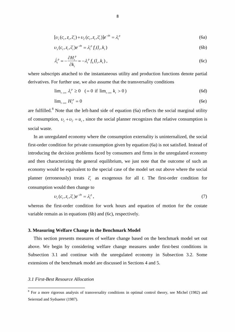
[ ( , , ) ( , , )] t pc t t t c t t t tc z c c z c e θu u l−+ = (6a)

( , , ) ( , )t pz t t t t l t tc z c e f l kθu l− = (6b)

( , )p

p ptt t k t t

t

H f l kk

l l∂= − = −

∂ , (6c)

where subscripts attached to the instantaneous utility and production functions denote partial

derivatives. For further use, we also assume that the transversality conditions

lim 0pt tl→∞ ≥ ( 0= if lim 0t tk→∞ > ) (6d)

lim 0pt tH→∞ = (6e)

are fulfilled.8 Note that the left-hand side of equation (6a) reflects the social marginal utility

of consumption, c c cuu u+ = , since the social planner recognizes that relative consumption is

social waste.

In an unregulated economy where the consumption externality is uninternalized, the social

first-order condition for private consumption given by equation (6a) is not satisfied. Instead of

introducing the decision problems faced by consumers and firms in the unregulated economy

and then characterizing the general equilibrium, we just note that the outcome of such an

economy would be equivalent to the special case of the model set out above where the social

planner (erroneously) treats tc as exogenous for all t. The first-order condition for

consumption would then change to

( , , ) t pc t t t tc z c e θu l− = , (7)

whereas the first-order condition for work hours and equation of motion for the costate

variable remain as in equations (6b) and (6c), respectively.

3. Measuring Welfare Change in the Benchmark Model

This section presents measures of welfare change based on the benchmark model set out

above. We begin by considering welfare change measures under first-best conditions in

Subsection 3.1 and continue with the unregulated economy in Subsection 3.2. Some

extensions of the benchmark model are discussed in Sections 4 and 5.

3.1 First-Best Resource Allocation

8 For a more rigorous analysis of transversality conditions in optimal control theory, see Michel (1982) and

Seierstad and Sydsaeter (1987).

9

As a point of departure, consider first the problem of measuring welfare change along the

first-best optimal path that obeys equations (6a)-(6c), where the externalities associated with

relative consumption concerns are fully internalized. This constitutes a natural reference case,

although it is presumably not very realistic. We use the superscript * to denote the socially

optimal resource allocation, such that

{ }* * * ,*, , , pt t t tc l k tl ∀

satisfy equations (4) and (6) along with the initial and terminal conditions for the capital

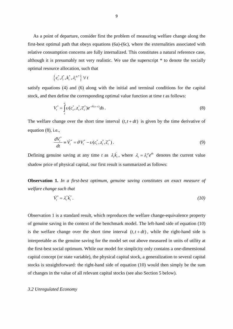
stock, and then define the corresponding optimal value function at time t as follows:

* * * * ( )( , , ) s tt s s s

t

V c z c e dsθu∞

− −= ∫ . (8)

The welfare change over the short time interval ( , )t t dt+ is given by the time derivative of

equation (8), i.e.,

*

* * * * *( , , )tt t t t t

dVV V c z c

dtθ u≡ = − . (9)

Defining genuine saving at any time t as t tkl , where p tt t eθl l= denotes the current value

shadow price of physical capital, our first result is summarized as follows:

Observation 1. In a first-best optimum, genuine saving constitutes an exact measure of

welfare change such that

* * *t t tV kl= . (10)

Observation 1 is a standard result, which reproduces the welfare change-equivalence property

of genuine saving in the context of the benchmark model. The left-hand side of equation (10)

is the welfare change over the short time interval ( , )t t dt+ , while the right-hand side is

interpretable as the genuine saving for the model set out above measured in units of utility at

the first-best social optimum. While our model for simplicity only contains a one-dimensional

capital concept (or state variable), the physical capital stock, a generalization to several capital

stocks is straightforward: the right-hand side of equation (10) would then simply be the sum

of changes in the value of all relevant capital stocks (see also Section 5 below).

3.2 Unregulated Economy

10

Here we analyze the probably more realistic case where the externalities associated with

relative consumption concerns are not internalized, implying that the first-order condition for

private consumption is given by equation (7) instead of equation (6a), and that equation (10)

is no longer valid. Let

{ }0 0 ,0, , pt t tc k tl ∀

denote the resource allocation in the unregulated economy, and let the corresponding value

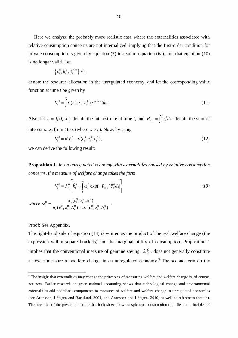
function at time t be given by

0 0 0 0 ( )( , , ) s tt s s s

t

V c z c e dsθu∞

− −= ∫ . (11)

Also, let ( , )t k t tr f l k= denote the interest rate at time t, and 0s

s t tR r dt t− = ∫ denote the sum of

interest rates from t to s (where s t> ). Now, by using

0 0 0 0 0( , , )t t t t tV V c z cθ u= − , (12)

we can derive the following result:

Proposition 1. In an unregulated economy with externalities caused by relative consumption

concerns, the measure of welfare change takes the form

0 0 0 0 0exp( )t t t s s t st

V k R c dsl α∞

−

= − −

∫ (13)

where 0 0 0

00 0 0 0 0 0

( , , )( , , ) ( , , )

t t tt

c t t t t t t

u c zu c z u c z

α ∆

∆

∆=

∆ + ∆.

Proof: See Appendix.

The right-hand side of equation (13) is written as the product of the real welfare change (the

expression within square brackets) and the marginal utility of consumption. Proposition 1

implies that the conventional measure of genuine saving, t tkl , does not generally constitute

an exact measure of welfare change in an unregulated economy.9 The second term on the

9 The insight that externalities may change the principles of measuring welfare and welfare change is, of course,

not new. Earlier research on green national accounting shows that technological change and environmental

externalities add additional components to measures of welfare and welfare change in unregulated economies

(see Aronsson, Löfgren and Backlund, 2004, and Aronsson and Löfgren, 2010, as well as references therein).

The novelties of the present paper are that it (i) shows how conspicuous consumption modifies the principles of

11

right-hand side is the value of the marginal externality and is given by a weighted sum of

discounted future changes in the reference consumption, where the instantaneous weights are

defined by the degrees of positionality along the economy’s equilibrium path. This component

is forward looking, since the welfare function at any time t is intertemporal and reflects future

utility.

Note that in the economy with identical individuals analyzed so far, c is always equal to c,

implying that their growth rates will also be the same. Thus, in a growing economy, the

second term on the right-hand side of equation (13) will be negative and genuine saving will

overestimate the welfare change. Also, the more positional the consumers are, i.e., the larger

the α , the greater the discrepancy between the conventional measure of genuine saving and

the welfare change, ceteris paribus. Therefore, empirical estimates of the degree of

positionality, along with estimates of changes in the average consumption, are important for

calculating the second term on the right-hand side of equation (13).

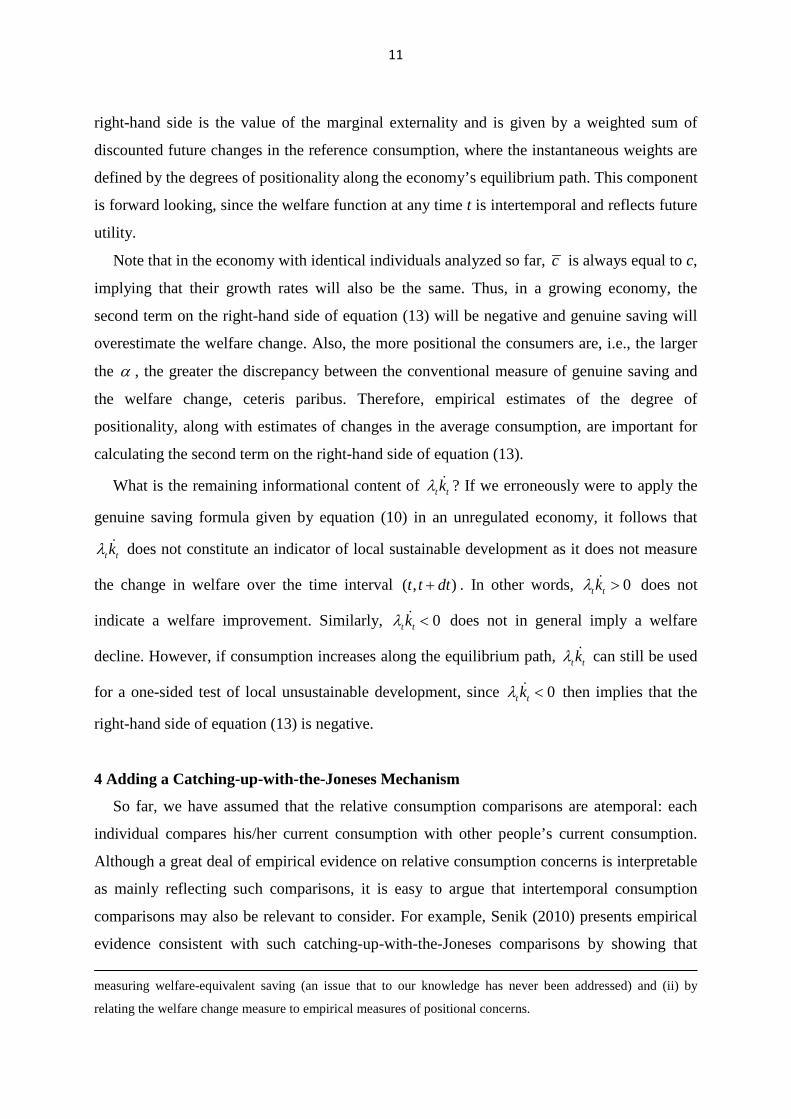
What is the remaining informational content of t tkl ? If we erroneously were to apply the

genuine saving formula given by equation (10) in an unregulated economy, it follows that

t tkl does not constitute an indicator of local sustainable development as it does not measure

the change in welfare over the time interval ( , )t t dt+ . In other words, 0t tkl > does not

indicate a welfare improvement. Similarly, 0t tkl < does not in general imply a welfare

decline. However, if consumption increases along the equilibrium path, t tkl can still be used

for a one-sided test of local unsustainable development, since 0t tkl < then implies that the

right-hand side of equation (13) is negative.

4 Adding a Catching-up-with-the-Joneses Mechanism

So far, we have assumed that the relative consumption comparisons are atemporal: each

individual compares his/her current consumption with other people’s current consumption.

Although a great deal of empirical evidence on relative consumption concerns is interpretable

as mainly reflecting such comparisons, it is easy to argue that intertemporal consumption

comparisons may also be relevant to consider. For example, Senik (2010) presents empirical

evidence consistent with such catching-up-with-the-Joneses comparisons by showing that measuring welfare-equivalent saving (an issue that to our knowledge has never been addressed) and (ii) by

relating the welfare change measure to empirical measures of positional concerns.

12

individual well-being is higher if the individual’s standard of living exceeds that of his/her

parents 15 years earlier, ceteris paribus. Such comparisons are also consistent with the

empirical pattern of various financial puzzles (Constantinides, 1990; Campbell and Cochrane,

1999; and Díaz et al., 2003). It is therefore clearly interesting to investigate whether the

qualitative results and interpretations presented in the previous section above carry over to a

framework where the individual also derives utility from comparisons with other people’s

past consumption. As will be shown, they essentially do.

There are at least two ways of modeling such intertemporal consumption comparisons.

One is to add a stock reflecting a weighted average of other people’s past consumption over

the entire history of the model, as Aronsson and Löfgren (2008) did in their study on the

comprehensive net national product under external habit formation. Another way is to assume

that the individual directly derives utility from comparing his/her time t consumption with

others’ consumption at time t ε− (and possibly other points in time as well). We use the latter

approach as it requires less modifications of the model set out above. The instantaneous utility

at time t is then rewritten to read

( , , , ) ( , , , )t t t t t t t t tU u c z c z c c εδ u −= ∆ = , (14)

where t t tc c εδ −= − denotes the individual’s relative consumption compared with others’ past

consumption. Thus, the instantaneous utility is no longer time separable. All other aspects of

the model remain as above.

We can then distinguish between the degree of atemporal positionality (which is analogous

to the positionality concept discussed above) and the degree of intertemporal positionality.10

By using equation (14), these two measures are summarized as

( , , , ) (0,1)( , , , ) ( , , , ) ( , , , )

t t t tt

c t t t t t t t t t t t t

u c zu c z u c z u c zδ

δαδ δ δ

∆

∆

∆= ∈

∆ + ∆ + ∆ (15)

( , , , ) (0,1)( , , , ) ( , , , ) ( , , , )

t t t tt

c t t t t t t t t t t t t

u c zu c z u c z u c z

δ

δ

δβδ δ δ∆

∆= ∈

∆ + ∆ + ∆. (16)

As before, tα denotes the degree of atemporal positionality (with the same interpretation as

equation (2) above) and tβ the degree of intertemporal positionality at time t. The latter

positionality concept measures the fraction of the utility gain of an additional dollar spent on

10 This distinction originates from Aronsson and Johansson-Stenman (2014), who analyze the simultaneous

implications of keeping-up-with-the-Joneses and catching-up-with-the-Joneses types of comparisons for optimal

taxation in an OLG model.

13

consumption that is due to increased relative consumption compared with other people’s past

consumption.

Consider first the socially optimal resource allocation. Here, since the reference

consumption measure on which the intertemporal consumption comparison is based enters the

instantaneous utility function with a time lag, equation (6a) is replaced with

( )[ ( , , , ) ( , , , )] ( , , , ) 0t t t

t t pc t t t t c t t t t c t t t t tc z c c c z c c e c z c c eθ θ ε

ε ε ε ε εu u u l− +− − + + ++ + − = , (17)

where the third term on the right-hand side is due to the delayed response mechanism caused

by intertemporal consumption comparisons. The other first-order conditions remain as in

equations (6b) and (6c). By using the same procedure as above, it is straightforward to show

that equation (10) in Observation 1 still applies, since there are no uninternalized externalities

that affect the welfare change measure, i.e., * * *t t tV kl= .

In the unregulated economy, the first-order conditions are also in this case given by

equations (6b), (6c), and (7), and we have the following analogue to Proposition 1:

Proposition 2. In an unregulated economy, where the externalities associated with relative

consumption concerns are driven by both keeping-up-with-the-Joneses and catching-up-with-

the-Joneses comparisons, the measure of welfare change takes the form

0 0 0 0 0 0 0exp( ) exp( )t t t s s t s s s t st t

V k R c ds R c dsε εl α β∞ ∞

− + + −

= − − − −

∫ ∫ . (18)

The interpretation of equation (18) is analogous to that of equation (13), with the only

modification that the value of the marginal externality is divided in two parts in equation (18).

The reason is, of course, that equation (18) is based on the assumption that there are two

mechanisms (a keeping-up and a catching-up mechanism) behind the relative consumption

comparisons. We can see that externalities associated with the keeping-up and catching-up

comparisons affect the welfare change measure in the same general way. Therefore, the

interpretations of Proposition 1 essentially carry over to Proposition 2. While this conclusion

is interesting per se, it also suggests that we may skip the catching-up component in what

follows in order to keep the model as simple and transparent as possible.

5. Public Investments

14

This section extends the benchmark model by analyzing the role of public investments.

The implications of relative consumption concerns for the optimal provision of public goods

have been addressed in several studies (e.g., Ng, 1987; Aronsson and Johansson-Stenman,

2008, forthcoming). Relative concerns for private consumption affect the optimal policy rule

for public good provision via two channels: (1) an incentive to internalize positional

externalities through increased public provision (which reduces the private consumption) and

(2) an (indirect) incentive to reduce the public provision as relative consumption concerns

lower the consumers’ marginal willingness to pay for public goods, ceteris paribus. As such,

whether or not positional preferences for private consumption influence the policy rule for a

public good largely depends on the preference elicitation format. In turn, this has a direct

bearing on the way public investment ought to be reflected in the context of genuine saving,

which motivates the following extension.

We will, consequently, add a public good of stock character to the instantaneous utility,

which means that equation (1) changes to

( , , , ) ( , , , )t t t t t t t t tU u c z g c z g cu= ∆ = , (19)

where tg denotes the level of the public good at time t (e.g., the state of the natural

environment). The public good accumulates through the following differential equation:11

t t tg q gg= − , (20)

where tq denotes the flow expenditure directed toward the public good at time t, i.e., the

instantaneous contribution, and g denotes the rate of depreciation. We also impose the initial

condition that 0g is fixed and the terminal condition lim 0t tg→∞ ≥ . Finally, since part of

output is used for contributions to the public good, the resource constraint slightly changes

such that

( , )t t t t tk f l k c qρ= − − , (21)

where ρ is interpretable as the (fixed) marginal rate of transformation between the public

good and the private consumption good.

11 Since the public good is interpretable in terms of environmental quality, a possible (and realistic) extension of

equation (20) would be to assume that increased output leads to lower environmental quality (instead of just

assuming a natural rate of depreciation). Yet, we refrain from this extension here as it is not important for the

qualitative results derived below.

15

These extensions mean that we have added the control variable q and the state variable g

to the benchmark model; otherwise, the model is the same as in Section 2. Thus, the social

decision problem is to choose tc , tl , and tq for all t to maximize the present value of future

utility,

0 0

( , , , )t tt t t t tU e dt c z g c e dtθ θu

∞ ∞− −=∫ ∫ ,

subject to equations (20) and (21) along with initial and terminal conditions. The present

value Hamiltonian can then be written as

( , , , ) [ ( , ) ] [ ]p t p pt t t t t t t t t t t t tH c z g c e f l k q c q gθu l ρ µ g−= + − − + − . (22)

The variable ptµ denotes the present value shadow price of the public good at time t, and its

current value counterpart is given by p tt t eθµ µ= . Note that equations (6a)-(6e), if written in

terms of the instantaneous utility function examined here (i.e., equation [19]), are necessary

conditions also in this extended model. In addition to (the modified) equations (6), the first-

order conditions for a social optimum also include an efficiency condition for q , an equation

of motion for pµ , and an additional transversality condition, i.e.,

p pt tl ρ µ= (23a)

( , , , )p

p t ptt g t t t t t

t

Hc z g c e

gθµ u µ g−∂

= − = − +∂

(23b)

lim 0pt tµ→∞ ≥ ( 0= if lim 0t tg→∞ > ). (23c)

Equations (6a)-(6e) and (23) characterize the social optimum. As in Subsections 3.1 and 3.2,

if the positional externality has not become internalized, equation (6a) should be replaced

with equation (7) (again modified to reflect the instantaneous utility function [19] that

contains the public good). For further use, let us also solve the differential equation (23b)

forward subject to the transversality condition (23c),12 which gives

(s t)( , , , )p st g s s s s

t

c z g c e e dsθ gµ u∞

− − −= ∫ . (24)

We are now ready to present the main results. As before, to separate the social optimum

from an allocation with uninternalized positional externalities, we use superscript * to denote

the socially optimal resource allocation and superscript 0 to denote the unregulated economy.

12 We assume that lim 0t tg→∞ > .

16

The value function (social welfare function) at any time t will be defined in the same way as

above, i.e.,

( )( , , , ) s tt s s s s

t

V c z g c e dsθu∞

− −= ∫ .

Then, by recognizing that genuine saving now reads t t t tk gl µ+ (since the capital concept is

two-dimensional here), we can use the same procedure as in Observation 1 and Proposition 1

to derive an analogue to equation (10) as follows:

* * * *t t t tV k gl ρ = +

, (25a)

and a corresponding analogue to equation (13):

0 0 0 0 0 0exp( )t t t t s s t st

V k g R c dsl ρ α∞

−

= + − −

∫ . (25b)

Except for the public investment component, equations (25a) and (25b) are interpretable in

exactly the same way as their counterparts in the simpler benchmark model, i.e., equations

(10) and (13).13

Equations (25a) and (25b) together imply the following treatment of public investment:

Proposition 3. Irrespective of whether the resource allocation is first best or represented by

an unregulated equilibrium, the accounting price of public investment is given by the

marginal rate of transformation between the public good and the private consumption good,

ρ .

Proposition 3 has a strong implication, as it means that the valuation of public investment

might be based on observables and that the same valuation procedure applies in a social

optimum and a distorted market economy. Although convenient, this result may seem

surprising at first sight. Yet, note that the information content in ρ differs between the two

regimes due to differences in the underlying policy rules for public provision. To see this

more clearly, let

13 If we extend the model by allowing ρ to vary over time, e.g., due to disembodied technological change, an

additional (forward-looking) term representing the marginal value of this technological change must be added to

equations (25a) and (25b).

17

g ggc

c c

uMRS

u uuu ∆

= =+

denote the marginal rate of substitution between the public good and private consumption

measured with the reference consumption, c , held constant, and

g ggc

c c c

uCMRS

uu

u u= =

+

denote the corresponding marginal rate of substitution measured with the relative

consumption, ∆ , held constant. Therefore, gcMRS refers to a conventional marginal

willingness to pay measure with other people’s consumption held constant. This means that

an increase in the public good will not only imply reduced (absolute) consumption, the

individual will also take into account the fact that his/her relative consumption decreases.

gcCMRS , on the other hand, reflects each respondent’s marginal willingness to pay for the

public good conditional on the fact that other people have to pay the same amount, implying

that relative consumption is held fixed. Thus, in this case there is no additional cost in terms

of reduced relative consumption, implying that under relative consumption concerns

gcCMRS will exceed gcMRS . Indeed, it is straightforward to show that

/ (1 )gc gcCMRS MRS α= − .

By using equations (6a), (23a), and (24), the policy rule for public provision in the first-

best optimum is then given by

**,( ( )) ( ( ))*

,* *1s t s ts gcR s t R s tt

s gct st t

MRSCMRS e ds e dsg gµ

ρl α

− −

∞ ∞− + − − + −= = =

−∫ ∫ , (26a)

while the corresponding policy rule implicit in the unregulated economy, based on equations

(7), (23a), and (24), becomes

0

( ( ))0,0

s tR s tts gc

t t

MRS e dsgµρ

l−

∞− + −= =∫ . (26b)

Equations (26a) and (26b) are different variants of the Samuelson condition for a state

variable public good. In a social optimum, where all positional externalities are internalized,

the social marginal rate of substitution between the public good and private consumption is

given by gcCMRS , which recognizes that relative consumption is pure waste. In the

unregulated economy, on the other hand, agents behave as if others’ consumption, c , is

exogenous, meaning that the marginal rate of substitution implicit in the first-order conditions

18

is given by gcMRS . In either case, however, it is optimal to equate the weighted sum of

marginal rates of substitution with the marginal rate of transformation, which explains

Proposition 3. There is an important practical implication here: regardless of whether we are

in a first-best economy or in an unregulated equilibrium, public investment can be valued by

the instantaneous marginal cost, such that there is no need to estimate future generations’

marginal willingness to pay for current additions to the public good.

6. Heterogeneity, Redistribution Policy and Genuine Saving

In the preceding sections we have consistently considered a representative-agent economy,

which is the typical framework used in earlier literature dealing with genuine saving. In this

section, we extend the analysis to a model where consumers are heterogeneous in terms of

productivity and productivity is private information. Such an extension is of course not

without costs in terms of greater complexity and less transparency. However, the benefits are

also considerable in terms of greater realism. In particular, it acknowledges the fact that there

is a social value of increased equality, and it also takes into account that redistributive taxes

are generally distortionary in the sense that they affect people’s incentive to work. This

framework, which is common in earlier literature on optimal taxation, has recently been used

to analyze the policy implications of relative consumption concerns. As explained in the

introduction, such an extension enables us to generalize the study of genuine saving to a

second-best economy where the social planner redistributes and internalizes externalities

subject to an incentive constraint.14

We make two simplifying assumptions. First, we do not consider public investments. Since

Proposition 3 can be shown to apply also in the model set out below, little additional insight

would be gained from studying such investments here as well. Second, to avoid unnecessary

technical complications with many different consumer types, we use the two-type setting

originally developed by Stern (1982) and Stiglitz (1982). The consumers differ in

productivity, and the high type (type 2) is more productive (measured in terms of the before-

14 To our knowledge, the paper by Aronsson, Cialani, and Löfgren (2012) is the only earlier study dealing with

genuine saving in a second-best economy with distortionary taxation. Their study is based on a representative-

agent model (and as such does not consider redistribution policy) and assumes that individuals only care about

their own absolute consumption and use of leisure (meaning that relative consumption is not dealt with at all).

19

tax wage rate) than the low type (type 1).15 The population is constant and normalized to one

for notational convenience, and there is a constant share, in , of individuals of type i, such that

1iin =∑ .

6.1 Preferences and Social Decision-Problem

We also allow for type-specific differences in preferences. The instantaneous utility

function facing each individual of type i can then be written as

( , , ) ( , , )i i i i i i i it t t t t t tU u c z c z cu= ∆ = , (27)

where ci it t tc∆ = − denotes the relative consumption of type i. The functions ( )iu ⋅ and ( )iu ⋅ in

equation (27) have the same general properties as their counterparts in equation (1). Also, and

similarly to the benchmark model presented in Section 2, the relative consumption concerns

in equation (27) solely reflect comparisons with other people’s current consumption, i.e., we

abstract from the catching-up mechanism briefly discussed above. The reference level is

assumed to be the average consumption in the economy as a whole, 1 1 2 2t t tc n c n c= + .16 As

before, each consumer is small relative to the overall economy and hence treats tc as

exogenous.

In a way similar to Sections 2 and 3, it is useful to be able to measure the extent to which

relative consumption matters for individual utility. By using the function ( )iu ⋅ in equation

(27), we can define the degree of positionality of type i at time t such that

( , , ) (0,1)( , , ) ( , , )

i i i ii t t tt i i i i i i i i

c t t t t t t

u c zu c z u c z

α ∆

∆

∆= ∈

∆ + ∆ for i=1,2, all t. (28)

Therefore, itα measures the fraction of the utility gain for type i at time t of increased

consumption that is due to increased relative consumption (compared with the reference

consumption level). 15 Aronsson (2010) uses a similar two-type model to derive a second-best analogue to the comprehensive net

national product. However, his study neither addresses the implications of relative consumption concerns nor

examines genuine saving, which are the main issues here. 16 This is the most common assumption in the literature dealing with optimal policy responses to relative

consumption concerns. Although the definition of reference consumption at the individual level (i.e., whether it

is based on the economy-wide mean value or reflects more narrow social reference groups) matters for public

policy, it is not equally important here, where the main purpose is to characterize an aggregate measure of social

savings.

20

Since we assume that all individuals compare their own consumption with the average

consumption in the economy as a whole, we can define the positional externality in terms of

the average degree of positionality. The average degree of positionality measured over all

individuals at time t can be written as (recall that the total population size is normalized to

unity)

1 1 2 2 (0,1)t t tn nα α α= + ∈ , (29)

which also reflects the sum of the marginal willingness to pay to avoid the positional

consumption externality measured per unit of consumption. Estimates of tα can be found in

empirical literature on relative consumption concerns, as discussed above (see the

introduction).

The social objective is assumed to be a general social welfare function

( )1 20

0

, tt tW U U e dtθω

∞−= ∫ . (30)

The instantaneous social welfare function, ( )ω ⋅ , is differentiable and increasing in the

instantaneous individual utilities. The resource constraint can now be written as

1 2( , , ) i it t t t ti

k f k n c= −∑ , (31)

where i i it tn l= is interpretable as the aggregate input of type i labor at time t. As before, the

production function, 1 2( , , )t t tf k , is characterized by constant returns to scale.

Following Aronsson and Johansson-Stenman (2010), we assume that the social planner (or

government) can observe labor income and saving at the individual level, while ability is

private information. We also assume that the social planner wants to redistribute from the

high type to the low type. To eliminate the incentive for the high type to mimic the low type

(in order to gain from this redistribution profile), we impose a self-selection constraint such

that each individual of the high type weakly prefers the allocation intended for his/her type

over the allocation intended for the low type. Also, to simplify the analysis, we assume that

the social planner commits to the resource allocation decided at time zero.17 One way to

rationalize this assumption in our framework is to interpret the model in terms of a continuum

of perfectly altruistic generations, i.e., dynasties (instead of single consumers with infinite

17 See Brett and Weymark (2008) for an analysis of optimal taxation without commitment based on the self-

selection approach to optimal taxation.

21

lives),18 such that the ability of agents living at any time t is not necessarily observable

beforehand by the social planner. Therefore, the self-selection constraint is assumed to take

the form

2 2 2 2 2 1 1 2ˆ( , , ) ( , , )t t t t t t t t tU c z c c l l c Uu u φ= ≥ − = (32)

for all t. The left-hand side represents the utility of the high type at time t and the right-hand

side the utility of the mimicker (a high type choosing the same income and saving as the low

type). The variable 1 21 2 1 2 1 2 1 2/ ( , , ) / ( , , ) ( , , ) 1t t t t t t t t t t t tw w f k f k kφ φ= = = <

denotes the

relative wage rate at time t, and 1 1t t tl lφ < is the hours of work the mimicking high type needs

to supply to reach the same labor income as the (mimicked) low type.

6.2 Second-Best Optimum and Genuine Saving

The social optimum can be derived by choosing 1tc , 1

tl , 2tc , and 2

tl for all t to maximize the

social welfare function given in equation (30), subject to the resource constraint and self-

selection constraint in equation (31) and (32), respectively, and to that the initial capital stock,

0k , is fixed and the terminal condition lim 0t tk→∞ ≥ . Also, the social planner recognizes that

the reference consumption is endogenous and given by 1 1 2 2t t tc n c n c= + .19 The present value

Hamiltonian at any time t is given by

( )1 2,p t pt t t t tH U U e kθω l−= + . (33)

Adding the self-selection constraint gives the present value Lagrangean 2 2ˆ[ ]p p p

t t t t tL H U Uη= + − , (34)

18 We realize that this interpretation is not unproblematic, since each individual in a succession of generations

faces his/her own objective and constraints; see Michel, Thibault, and Vidal (2006) for a discussion. However,

our main concern here is to examine the implications of the self-selection constraint for how positional

externalities ought to be treated in savings-based measures of welfare change. Since the externality is atemporal

in our model (i.e., a keeping-up-with-the-Joneses externality), the exact way in which successive generations

interact is of no major importance for the qualitative results. 19 We will not go into how such an allocation can be implemented by optimal nonlinear taxation. Here, the

reader is referred to Aronsson and Johansson-Stenman (2010). Other literature on optimal taxation under relative

consumption concerns includes Boskin and Sheshinski (1978), Oswald (1983), Corneo and Jeanne (1997, 2001),

Ireland (2001), Dupor and Liu (2003), Wendner and Goulder (2008), and Aronsson and Johansson-Stenman

(2014).

22

where ptη denotes the present value Lagrange multiplier. If written in terms of the reduced

form utility formulation ( )iu ⋅ in equation (27), and by using 2 2 1 1ˆ ( , , )t t t t tc l l cu u φ= − as a short

notation for the instantaneous utility facing the mimicker at time t, the first-order conditions

can be written as (in addition to equations [31] and [32] and the initial and terminal conditions

for the capital stock)

11 2 1 1

1ˆ 0

p pt p p

c cU

L Le n nc c

θω u η u l−∂ ∂= − − + =

∂ ∂ (35a)

11 2 1 1 1

1 1ˆ [ ] 0

pt p p

z zU

L e l n wl l

θ φω u η u φ l−∂ ∂= − + + + =

∂ ∂ (35b)

22 2 2 2

2 0p p

t p pc cU

L Le n nc c

θω u η u l−∂ ∂= + − + =

∂ ∂ (35c)

22 2 2 1 2 2

2 2ˆ[ ] 0

pt p p

z z zU

L e l n wl l

θ φω u η u u l−∂ ∂= − + − + + =

∂ ∂ (35d)

2 1ˆp

p pp z

L r lk k

φl l η u∂ ∂= − = − −

∂ ∂ . (35e)

The optimal resource allocation also fulfills transversality conditions analogous to equations

(6d) and (6e). In equations (35), we have suppressed the time indicator to avoid notational

clutter (since all components refer to the same point in time), and subscripts attached to the

instantaneous utility functions and social welfare function refer to partial derivatives (as

before). The factor prices are determined by marginal products, i.e., 11 1 2( , , )w f k=

,

22 1 2( , , )w f k=

, and 1 2( , , )kr f k= .

The final term on the right-hand side of equations (35a) and (35c) reflects the positional

consumption externality and measures the partial instantaneous welfare effect of increased

reference consumption times the effect of each type’s consumption on the reference measure.

This partial welfare effect can be either positive or negative and is given as follows:

1 21 2 2 2, , , ,ˆ

t t t tt t

Pt t pt

t c t c t t c t cU Ut

L e ec

θ θω u ω u η u u− −∂ = + + − ∂. (36)

Although the first two terms on the right-hand side are negative, since , 0t

it cu < for i=1,2 by

the assumptions made earlier, the third term (which is proportional to the Lagrange multiplier

of the self-selection constraint) can be either positive or negative. We will return to equation

(36) in greater detail below.

23

We are now ready to derive a measure of welfare change for the second-best economy set

out above. The main differences compared with the model analyzed in Sections 2 and 3 are

that (i) the individuals differ in productivity and preferences here, meaning also that they may

differ in terms of relative consumption concerns (see equation [28] above), (ii) the social

planner has an objective that may necessitate redistribution policy, and (iii) the social planner

is unable to implement the first-best resource allocation (provided that the self-selection

constraint binds). Despite these differences, we will also in this case use the superscript * to

denote social optimum (let be a second-best optimum) such that

{ }1,* 1,* 2,* 2,* * ,*, , , , , pt t t t t tc l c l k tl ∀

satisfy equations (6d), (6e), (31), (32), and (35a)-(35e) as well as the initial and terminal

conditions. The optimal value function at time t (based on the social welfare function) then

becomes

( )* 1,* 1,* * 2,* 2,* * ( )( , , ), ( , , ) s tt s s s s s s

t

W c z c c z c e dsθω u u∞

− −= ∫ . (37)

We can then derive the following strong result regarding the change in social welfare over

a short time interval, ( , )t t dt+ :

Proposition 4. If the resource allocation satisfies equations (6d), (6e), (31), and (35a)-(35e),

and irrespective of whether the self-selection constraint binds, genuine saving constitutes an

exact measure of social welfare change such that

* * *t t tW kl= , (38)

where * ,*p tt t eθl l= .


Proposition 4 constitutes a remarkable result. It means that the procedure for measuring

welfare change in a first-best representative-agent economy (as discussed in Section 3) carries

over to the second-best economy analyzed here, where the agents differ in productivity

(which is private information). The only difference is that the shadow price of capital is

measured in a slightly different way (which is seen by comparing equations [6c] and [35e]).

The intuition is that the redistribution is optimal given the social welfare function and

constraints, and the positional externality is internalized. As a consequence, there is no market

failure or failure to reach the distributional objectives that may cause a discrepancy between

24

the welfare change and the conventional measure of genuine saving.20 This holds true

irrespective of whether the resource allocation is first best or second best.

6.3 Welfare Change and Positional Externalities

To be able to focus on the welfare contributions of uninternalized externalities, we model

the unregulated economy in the same general way as above by assuming that the resource

allocation is optimal conditional on the level of reference consumption. In the context of the

present model, this means that the redistribution policy is decided in the same general way as

before with one exception: the social planner (erroneously) treats tc as exogenous. A possible

interpretation is that the income tax system is optimal conditional on tc , i.e., the underlying

tax policy is chosen as if the consumer preference for relative consumption does not give rise

to externalities.

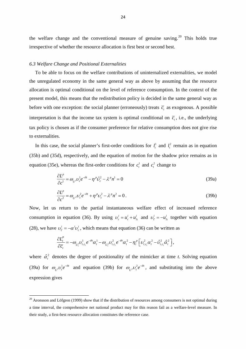
In this case, the social planner’s first-order conditions for 1tl and 2

tl remain as in equation

(35b) and (35d), respectively, and the equation of motion for the shadow price remains as in

equation (35e), whereas the first-order conditions for 1tc and 2

tc change to

11 2 1

1ˆ 0

pt p p

c cU

L e nc

θω u η u l−∂= − − =

∂ (39a)

22 2 2

2 0p

t p pc cU

L e nc

θω u η u l−∂= + − =

∂. (39b)

Now, let us return to the partial instantaneous welfare effect of increased reference

consumption in equation (36). By using i i ic cu uu ∆= + and i i

c uu ∆= − together with equation

(28), we have i i ic cu α u= − , which means that equation (36) can be written as

1 21 1 2 2 2 2 2 2, , , ,ˆ ˆ

t t t tt t

Pt t pt

t c t t c t t t c t t c tU Ut

L e ec

θ θω u α ω u α η u α u α− −∂ = − − − − ∂,

where 2ˆtα denotes the degree of positionality of the mimicker at time t. Solving equation

(39a) for 11 tcUe θω u − and equation (39b) for 2

2 tcUe θω u − , and substituting into the above

expression gives

20 Aronsson and Löfgren (1999) show that if the distribution of resources among consumers is not optimal during

a time interval, the comprehensive net national product may for this reason fail as a welfare-level measure. In

their study, a first-best resource allocation constitutes the reference case.

25

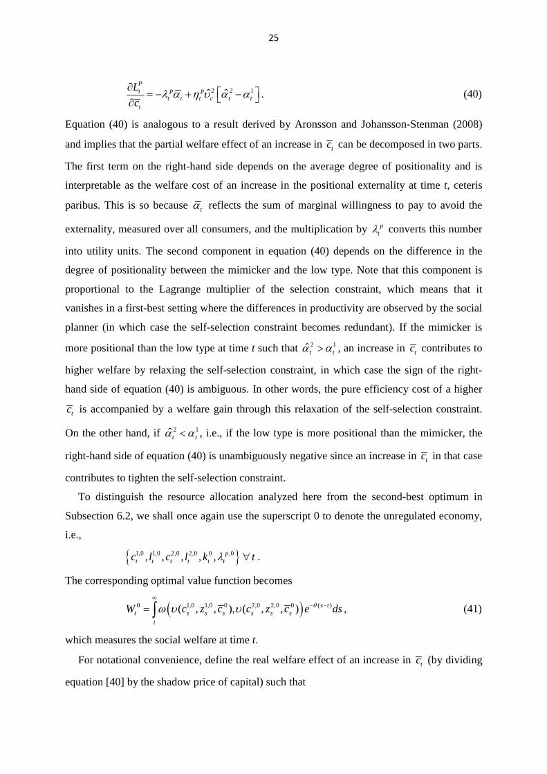
2 2 1ˆ ˆP

p ptt t t c t t

t

Lc

l α η u α α∂ = − + − ∂. (40)

Equation (40) is analogous to a result derived by Aronsson and Johansson-Stenman (2008)

and implies that the partial welfare effect of an increase in tc can be decomposed in two parts.

The first term on the right-hand side depends on the average degree of positionality and is

interpretable as the welfare cost of an increase in the positional externality at time t, ceteris

paribus. This is so because tα reflects the sum of marginal willingness to pay to avoid the

externality, measured over all consumers, and the multiplication by ptl converts this number

into utility units. The second component in equation (40) depends on the difference in the

degree of positionality between the mimicker and the low type. Note that this component is

proportional to the Lagrange multiplier of the selection constraint, which means that it

vanishes in a first-best setting where the differences in productivity are observed by the social

planner (in which case the self-selection constraint becomes redundant). If the mimicker is

more positional than the low type at time t such that 2 1ˆt tα α> , an increase in tc contributes to

higher welfare by relaxing the self-selection constraint, in which case the sign of the right-

hand side of equation (40) is ambiguous. In other words, the pure efficiency cost of a higher

tc is accompanied by a welfare gain through this relaxation of the self-selection constraint.

On the other hand, if 2 1ˆt tα α< , i.e., if the low type is more positional than the mimicker, the

right-hand side of equation (40) is unambiguously negative since an increase in tc in that case

contributes to tighten the self-selection constraint.

To distinguish the resource allocation analyzed here from the second-best optimum in

Subsection 6.2, we shall once again use the superscript 0 to denote the unregulated economy,

i.e.,

{ }1,0 1,0 2,0 2,0 0 ,0, , , , , pt t t t t tc l c l k tl ∀ .

The corresponding optimal value function becomes

( )0 1,0 1,0 0 2,0 2,0 0 ( )( , , ), ( , , ) s tt s s s s s s

t


− −= ∫ , (41)

which measures the social welfare at time t.

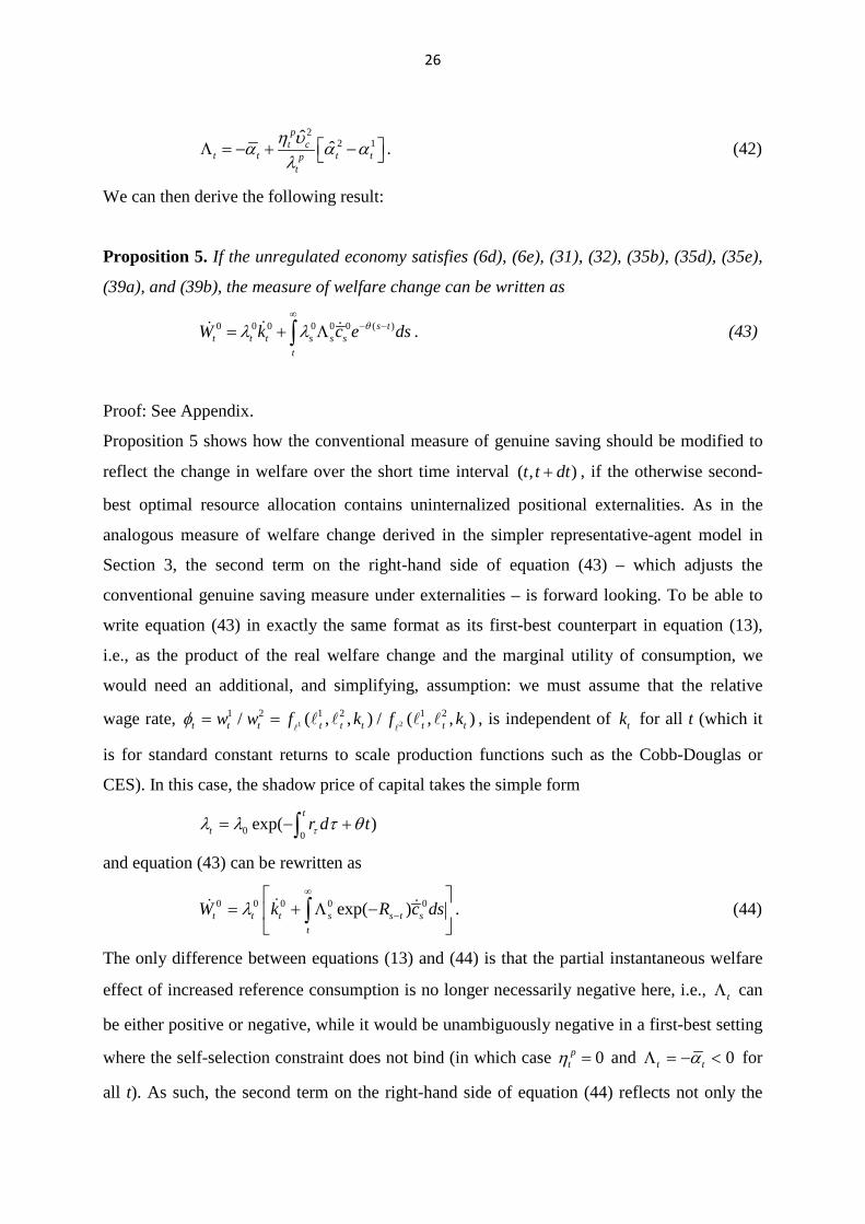
For notational convenience, define the real welfare effect of an increase in tc (by dividing

equation [40] by the shadow price of capital) such that

26

22 1ˆ ˆ

pt c

t t t tpt

η uα α αl

Λ = − + − . (42)

We can then derive the following result:

Proposition 5. If the unregulated economy satisfies (6d), (6e), (31), (32), (35b), (35d), (35e),

(39a), and (39b), the measure of welfare change can be written as

0 0 0 0 0 0 ( )s tt t t s s s

t

W k c e dsθl l∞

− −= + Λ∫ . (43)


Proposition 5 shows how the conventional measure of genuine saving should be modified to

reflect the change in welfare over the short time interval ( , )t t dt+ , if the otherwise second-

best optimal resource allocation contains uninternalized positional externalities. As in the

analogous measure of welfare change derived in the simpler representative-agent model in

Section 3, the second term on the right-hand side of equation (43) – which adjusts the

conventional genuine saving measure under externalities – is forward looking. To be able to

write equation (43) in exactly the same format as its first-best counterpart in equation (13),

i.e., as the product of the real welfare change and the marginal utility of consumption, we

would need an additional, and simplifying, assumption: we must assume that the relative

wage rate, 1 21 2 1 2 1 2/ ( , , ) / ( , , )t t t t t t t t tw w f k f kφ = =

, is independent of tk for all t (which it

is for standard constant returns to scale production functions such as the Cobb-Douglas or

CES). In this case, the shadow price of capital takes the simple form

0 0exp( )

t

t r d ttl l t θ= − +∫

and equation (43) can be rewritten as

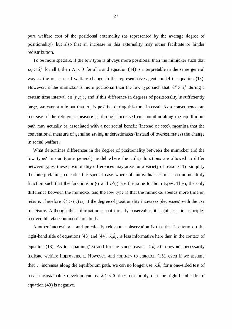
0 0 0 0 0exp( )t t t s s t st

W k R c dsl∞

−

= + Λ −

∫ . (44)

The only difference between equations (13) and (44) is that the partial instantaneous welfare

effect of increased reference consumption is no longer necessarily negative here, i.e., tΛ can

be either positive or negative, while it would be unambiguously negative in a first-best setting

where the self-selection constraint does not bind (in which case 0ptη = and 0t tαΛ = − < for

all t). As such, the second term on the right-hand side of equation (44) reflects not only the

27

pure welfare cost of the positional externality (as represented by the average degree of

positionality), but also that an increase in this externality may either facilitate or hinder

redistribution.

To be more specific, if the low type is always more positional than the mimicker such that 1 2ˆt tα α> for all t, then 0tΛ < for all t and equation (44) is interpretable in the same general

way as the measure of welfare change in the representative-agent model in equation (13).

However, if the mimicker is more positional than the low type such that 2 1ˆt tα α> during a

certain time interval 1 2( , )t t t∈ , and if this difference in degrees of positionality is sufficiently

large, we cannot rule out that tΛ is positive during this time interval. As a consequence, an

increase of the reference measure tc through increased consumption along the equilibrium

path may actually be associated with a net social benefit (instead of cost), meaning that the

conventional measure of genuine saving underestimates (instead of overestimates) the change

in social welfare.

What determines differences in the degree of positionality between the mimicker and the

low type? In our (quite general) model where the utility functions are allowed to differ

between types, these positionality differences may arise for a variety of reasons. To simplify

the interpretation, consider the special case where all individuals share a common utility

function such that the functions ( )iu ⋅ and ( )iu ⋅ are the same for both types. Then, the only

difference between the mimicker and the low type is that the mimicker spends more time on

leisure. Therefore 2 1ˆ ( )t tα α> < if the degree of positionality increases (decreases) with the use

of leisure. Although this information is not directly observable, it is (at least in principle)

recoverable via econometric methods.

Another interesting – and practically relevant – observation is that the first term on the

right-hand side of equations (43) and (44), t tkl , is less informative here than in the context of

equation (13). As in equation (13) and for the same reason, 0t tkl > does not necessarily

indicate welfare improvement. However, and contrary to equation (13), even if we assume

that tc increases along the equilibrium path, we can no longer use t tkl for a one-sided test of

local unsustainable development as 0t tkl < does not imply that the right-hand side of

equation (43) is negative.

28

7. Numerical Illustration

In previous sections, we have shown that conventional measures of genuine saving do not

generally constitute valid measures of welfare change, and we have also derived exact welfare

change measures for unregulated economies. While this is important per se, it is also

important to be able to say something about likely orders of magnitude and whether or not the

modifications are likely to be similar between countries in percentage terms. In this section

we illustrate first that the discrepancies between measures of genuine saving and welfare

change are indeed likely to be substantial and second that these modifications may also differ

greatly between countries.

Our numerical simulation example is based on data for Sweden and the U.S., and serves to

provide a rough estimate of the right-hand side of equation (44), i.e., the genuine saving

adjusted for uninternalized positional externalities. To be able to manage this task without a

lengthy numerical extension of the paper, we make four additional, simplifying assumptions:

(i) all consumers share a common utility function where leisure is weakly separable from the

other goods, (ii) the positionality degree is constant over time for all consumers, (iii) the

interest rate is constant over time, and (iv) the average consumption in the economy can be

approximated by a consumption function with a constant growth rate.

Assumption (i) means that the mimicker and the mimicked agent are equally positional,

i.e., 2 1ˆt tα α= , implying, in turn, that the second term on the right-hand side of equation (42)

vanishes.21 This does not in itself require that all individuals are equally positional; the model

is still consistent with differences in positional concerns among types. Taken together,

assumptions (i) and (ii) imply t tα αΛ = − = − for all t,22 while assumption (iii) implies tr r=

for all t. Finally, assumption (iv) is consistent with models used in literature on endogenous

growth and implies that we can write the average consumption at any time s t> as

( )s ts tc c eκ −= , (45)

where κ is the growth rate.

21 To our knowledge, there is no empirical evidence available here, which suggests that the relationship between

the degree of consumption positionality and the use of leisure is a relevant issue for future research. Therefore,

lack of empirical evidence on this relationship motivates us to assume leisure separability. 22 Assumption (ii) can alternatively be replaced with a functional form assumption on the instantaneous utility

function, such that the degree of positionality is constant over time; see, e.g., Ljunqvist and Uhlig (2000).

29

Our aim is now to operationalize the welfare change measure for the unregulated economy

given in equation (44). As such, the calculations below presuppose that the positional

externality is uninternalized, while all other aspects of public policy are optimally chosen

conditional on the level of reference consumption. By using assumptions (i)-(iv), equation

(44) can be written in the following convenient way:23

1 exp( )t t s s t st t

t tGS

ME

W k R c ds

k cr

lακκ

∞

−= + Λ −

= −−

∫

. (46)

The left-hand side of equation (46) is a money-metrics version of the welfare change (through

division by the marginal utility of consumption), while the right-hand side decomposes this

into the conventional genuine saving (GS) and the value of the marginal externality (ME). In

particular, note that the higher the average degree of positionality, α , or the higher the

consumption growth rate, κ , ceteris paribus, the larger the marginal externality will be, and

the more the conventional measure of genuine saving will overestimate the welfare change.

To estimate equation (46), we use data from Sweden and the U.S. for the period 1990-

2012. Our point of departure is the World Bank measure of adjusted net saving, which we

interpret as a conventional indicator of genuine saving that does not reflect any positional

externalities (i.e., our GS above).24 We shall then examine how this measure ought to be

modified in response to uninternalized positional externalities through the second term on the

right-hand side of equation (46). The raw data contains information on the adjusted net

saving, aggregate private consumption, total population, and the GDP deflator, allowing us to

calculate both the conventional genuine saving and the value of the marginal externality in

23 Since assumption (i) eliminates any difference in the degree of positionality between the mimicker and the low

type, the second line of equation (46) would also follow from the welfare change measure of the representative-

agent model given in equation (13). 24 The adjusted net saving is defined as the net national savings plus education expenditure minus an

estimated value of energy depletion, mineral depletion, forest depletion, carbon dioxide emissions, and

particulate emissions damage. We realize, of course, that this definition captures several aspects not addressed

above (mainly referring to valuation of human capital and environmental capital). Yet, our more narrow

definition of net investment is not important here, since adding investments in human and environmental capital

does not affect any of the qualitative results derived above. In fact, we showed in Section 5 that a straightforward

extension of the model would allow us to reinterpret k to reflect a broader capital concept.

30

real per capita terms.25 We use per capita variables to avoid possible welfare consequences of

population size and growth (which we have abstracted from above). The average degree of

positionality is assumed to be in the interval 0.2-0.4, which is thus a conservative assumption

given the empirical research discussed in the introduction. The calculations are presented in

Table 1.

Table 1 HERE

The numbers in Table 1 should be seen for what they are, i.e., the outcome of a

computational example and not the result of empirical research. With this reservation in mind,

we would nevertheless like to emphasize three important insights from the table. First, the

value of the marginal externality is substantial. Note that this is so despite our quite

conservative estimates of the average degree of positionality, α . Indeed, even based on the

lower-bound estimate of 0.2, we obtain quite large values of the marginal externality. This

suggests that the conventional measure of genuine saving may largely overestimate the true

welfare change. Second, the conventional measure of genuine saving may give incorrect

qualitative information as to whether the development is locally sustainable. For several

combinations of growth rate, interest rate, and average degree of positionality, GS-ME is less

than zero despite that GS is positive. Third, this discrepancy will generally not be similar

between countries. In our case, the discrepancy is considerably larger for the U.S. than for

Sweden, as the conventional genuine saving is smaller and the per capita consumption larger

in the U.S. than in Sweden.

8. Discussion and Conclusion

This paper deals with the measurement of welfare change by developing an analogue to

genuine saving in an economy where the consumers are positional. Recent empirical evidence

shows that people derive utility from their own consumption relative to that of referent others,

and also that the negative externalities of this wasteful consumption might be substantial,

implying that measures of social savings ought to be modified accordingly. This is further

emphasized by the now widely accepted role that genuine saving plays as an indicator of local

sustainable development. 25 These data are from the database World Development Indicators of the World Bank:

http://data.worldbank.org/data-catalog/world-development-indicators.

31

In the context of first-best representative-agent economies, earlier research shows that the

genuine saving is an exact indicator of welfare change and also interpretable as an exact

indicator of local sustainable development. We show that this result carries over to a second-

best economy based on asymmetric information about individual productivity and a binding

self-selection constraint, in the sense that the change in social welfare (measured by a general

social welfare function) over a short time interval is exactly equal to the genuine saving. We

also show how the value of public investment affects genuine saving and derive a simple

accounting price that applies irrespective of whether or not the positional externalities have

become internalized.

However, in the arguably more interesting case where the positional externality has not

become fully internalized, the equality between welfare change and genuine saving no longer

applies, and we show how this discrepancy depends on the degrees of positionality (i.e.,

measures used in empirical literature to indicate the extent to which relative consumption

matters for individual well-being). In a representative-agent model, and if the consumption

increases along the general equilibrium path (which the ideas of a positional arms race may

suggest), uninternalized positional externalities typically imply that the genuine saving

overestimates the change in social welfare. As such, negative genuine saving can still be used

as an indicator of local unsustainable development, i.e., negative genuine saving implies that

the social welfare declines.

In an economy with productivity differences and asymmetric information, the conventional

measure of genuine saving is even less informative if the positional externalities are not

internalized. If this is the case, negative genuine saving can no longer be used as an indicator

of local unsustainable development. We also demonstrate in a numerical exercise that the

modifications are likely to be substantial and that they are likely to differ between countries to

a large extent.

Future research may take several possible directions. First, recent empirical evidence

shows that individuals do not only compare their own consumption with that of other

domestic residents, they also engage in between-country comparisons (Becchetti et al., 2013).

This suggests to us that a multi-country framework might be useful in future research on

genuine saving. We conjecture that genuine saving is less useful as an indicator of welfare

change at the national level in such a setting. Second, although empirical evidence shows that

people are concerned with their relative consumption, people are also found to have an

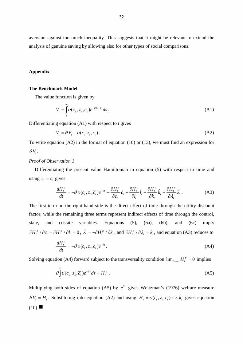
32

aversion against too much inequality. This suggests that it might be relevant to extend the

analysis of genuine saving by allowing also for other types of social comparisons.

Appendix

The Benchmark Model

The value function is given by

( )( , , ) s tt s s s

t

V c z c e dsθu∞

− −= ∫ . (A1)

Differentiating equation (A1) with respect to t gives

( , , )t t t t tV V c z cθ u= − . (A2)

To write equation (A2) in the format of equation (10) or (13), we must find an expression for

tVθ .

Proof of Observation 1

Differentiating the present value Hamiltonian in equation (5) with respect to time and

using t tc c= gives

( , , )p p p p p

tt t t t tt t t t t t t

t t t t

dH H H H Hc z c e c l k

dt c l kθθ u l

l− ∂ ∂ ∂ ∂

= − + + + +∂ ∂ ∂ ∂

. (A3)

The first term on the right-hand side is the direct effect of time through the utility discount

factor, while the remaining three terms represent indirect effects of time through the control,

state, and costate variables. Equations (5), (6a), (6b), and (6c) imply

/ / 0p pt t t tH c H l∂ ∂ = ∂ ∂ = , /p

t t tH kl = −∂ ∂ , and /pt t tH kl∂ ∂ = , and equation (A3) reduces to

( , , )p

ttt t t

dHc z c e

dtθθ u −= − . (A4)

Solving equation (A4) forward subject to the transversality condition lim 0pt tH→∞ = implies

( , , ) s ps s s t

t

c z c e ds Hθθ u∞

− =∫ . (A5)

Multiplying both sides of equation (A5) by teθ gives Weitzman’s (1976) welfare measure

t tV Hθ = . Substituting into equation (A2) and using ( , , )t t t t t tH c z c ku l= + gives equation

(10).

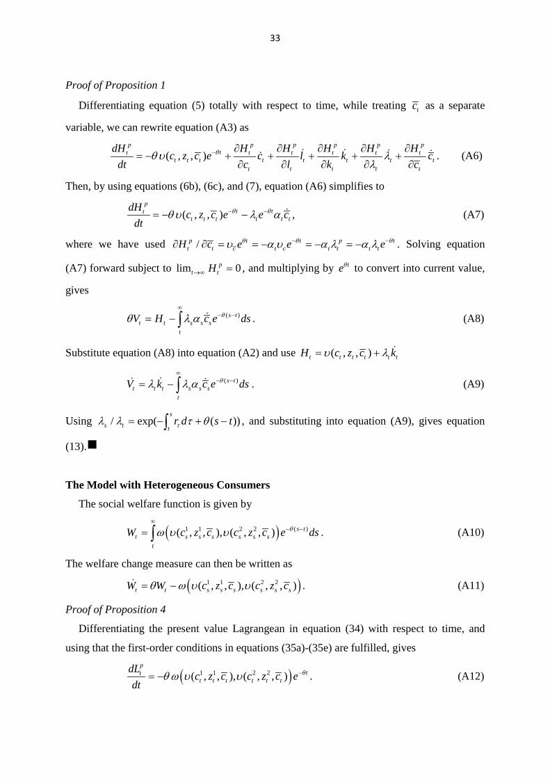
33

Proof of Proposition 1

Differentiating equation (5) totally with respect to time, while treating tc as a separate

variable, we can rewrite equation (A3) as

( , , )p p p p p p

tt t t t t tt t t t t t t t

t t t t t

dH H H H H Hc z c e c l k c

dt c l k cθθ u l

l− ∂ ∂ ∂ ∂ ∂

= − + + + + +∂ ∂ ∂ ∂ ∂

. (A6)

Then, by using equations (6b), (6c), and (7), equation (A6) simplifies to

( , , )p

t ttt t t t t t

dHc z c e e c

dtθ θθ u l α− −= − − , (A7)

where we have used /p t t p tt t c t c t t t tH c e e eθ θ θu α u α l α l− −∂ ∂ = = − = − = − . Solving equation

(A7) forward subject to lim 0pt tH→∞ = , and multiplying by teθ to convert into current value,

gives

( )s tt t s s s

t

V H c e dsθθ l α∞

− −= − ∫ . (A8)

Substitute equation (A8) into equation (A2) and use ( , , )t t t t t tH c z c ku l= +

( )s tt t t s s s

t

V k c e dsθl l α∞

− −= − ∫ . (A9)

Using / exp( ( ))s

s t tr d s ttl l t θ= − + −∫ , and substituting into equation (A9), gives equation

(13).

The Model with Heterogeneous Consumers

The social welfare function is given by

( )1 1 2 2 ( )( , , ), ( , , ) s tt s s s s s s

t


− −= ∫ . (A10)

The welfare change measure can then be written as

( )1 1 2 2( , , ), ( , , )t t s s s s s sW W c z c c z cθ ω u u= − . (A11)


Differentiating the present value Lagrangean in equation (34) with respect to time, and

using that the first-order conditions in equations (35a)-(35e) are fulfilled, gives

( )1 1 2 2( , , ), ( , , )p

ttt t t t t t

dLc z c c z c e

dtθθ ω u u −= − . (A12)

34

By solving equation (A12) in the same way as we solved equation (A4) above, and using that p pt tL H= , the proof follows by analogy to the proof of Proposition 1.


Differentiating the present value Lagrangean in equation (34) with respect to time, while

using the first-order conditions in equations (35c), (35d), (35e), (39a), and (39b), gives

( )1 1 2 2( , , ), ( , , )p

t ttt t t t t t t t t

dLc z c c z c e e c

dtθ θθ ω u u l− −= − + Λ , (A13)

where we have used /p p tt t t t t tL c e θl l −∂ ∂ = Λ = Λ . Solving equation (A13) forward subject to

the transversality condition lim 0pt tH→∞ = , using p p

t tL H= , and multiplying by te θ− to

convert into current value terms, gives

( )1 1 2 2 ( ) ( )( , , ), ( , , ) s t s ts s s s s s t s s s

t t

c z c c z c e ds H c e dsθ θθ ω u u l∞ ∞

− − − −= + Λ∫ ∫ . (A14)

Substituting into equation (A11) and using ( )1 2,t t t t tH U U kω l= + gives equation (43).

References

Akerlof, G. A. (1997) Social Distance and Social Decisions. Econometrica 65, 1005-1027.

Alpizar, F., F. Carlsson and O. Johansson-Stenman (2005) How Much Do We Care About

Absolute versus Relative Income and Consumption? Journal of Economic Behavior and

Organization 56, 405-421.

Aronsson, T. (2010) Welfare Measurement and Public Goods in a Second Best Economy. In

Aronsson, T. and Löfgren, K-G. (eds) Handbook of Environmental Accounting. Edward

Elgar Publishing Limited.

Aronsson, T., Cialani, C. and Löfgren, K-G. (2012) Genuine Saving and the Social Cost of

Taxation. Journal of Public Economics 96, 211-217.

Aronsson, T. and O. Johansson-Stenman (2008) When the Joneses’ Consumption Hurts:

Optimal Public Good Provision and Nonlinear Income Taxation. Journal of Public

Economics 92, 986-997.

Aronsson, T. and O. Johansson-Stenman (2010) Positional Concerns in an OLG Model:

Optimal Labor and Capital Income Taxation. International Economic Review 51, 1071-

1095.

35

Aronsson, T. and O. Johansson-Stenman (2014) Positional Preferences in Time and Space:

Optimal Income Taxation with Dynamic Social Comparisons. Journal of Economic

Behavior and Organization 101, 1-23.

Aronsson, T. and O. Johansson-Stenman (forthcoming) State-Variable Public Goods and

Social Comparisons. Journal of Environmental Economics and Management.

Aronsson, T. and Löfgren, K-G. (1999) Welfare Equivalent NNP under Distributional

Objectives. Economics Letters 63, 239-243.

Aronsson, T. and Löfgren, K-G. (2008) Welfare Equivalent NNP and Habit Formation.

Economics Letters 98, 84-88.

Aronsson, T. and Löfgren, K-G. (2010) An Introduction to the Theory of Social Accounting.

In Aronsson, T. and Löfgren, K-G. (eds) Handbook of Environmental Accounting.

Edward Elgar Publishing Limited.

Aronsson, T., Löfgren, K-G. and Backlund, K. (2004) Welfare Measurement in Imperfect

Markets: A Growth Theoretical Approach. Edward Elgar Publishing Limited.

Arrow, K. J., Dasgupta, P. and Mäler, K-G. (2003) Evaluating Projects and Assessing

Sustainable Development in Imperfect Economies. Environmental and Resource


Asheim, G.B. (1994) Net National Product as an Indicator of Sustainability. Scandinavian

Journal of Economics 96, 257-265.

Asheim, G. B. (2004) Green National Accounting with a Changing Population. Economic

Theory 23, 601-619.

Becchetti, L., S. Castriota and E. Giachin Ricca (2013) Beyond the Joneses: Inter-Country

Income Comparisons and Happiness. Journal of Socio-Economics 45, 187-196.

Boskin, M. J. and E. Sheshinski (1978) Individual Welfare Depends upon Relative Income.

Quarterly Journal of Economics 92, 589-601.

Campbell, J. Y., Cochrane, J. H., (1999) By Force of Habit: A Consumption-Based

Explanation of Aggregate Stock Market Behavior. Journal of Political Economy 107,

205-251.

Carlsson, F., O. Johansson-Stenman and P. Martinsson (2007) Do You Enjoy Having More

Than Others? Survey Evidence of Positional Goods. Economica 74, 586-598.

Clark, A.E. and C. Senik (2010) Who Compares to Whom? The Anatomy of Income

Comparisons in Europe. Economic Journal 120: 573-594.

36

Clark, A.E., and Senik, C. (2011) Will GDP Growth Increase Happiness in Developing

Countries? In R. Peccoud (Ed.), Measure For Measure: How Well Do We Measure

Development? Paris: STIN.

Constantinides, G. M., (1990) Habit Formation: A Resolution of the Equity Premium Puzzle.

Journal of Political Economy 98, 519-543.

Corazzini, L., Esposito, L. and F. Majorano (2012) Reign in Hell or Serve in Heaven? A

Cross-country Journey into the Relative vs Absolute Perceptions of Wellbeing. Journal

of Economic Behavior and Organization 81(3), 715-730.

Corneo, G. and O. Jeanne (1997) Conspicuous Consumption, Snobbism and Conformism.

Journal of Public Economics 66, 55-71.

Corneo, G., and O. Jeanne (2001) Status, the Distribution of Wealth, and Growth.

Scandinavian Journal of Economics 103, 283-293.

Díaz, A., Pijoan-Mas, J., Ríos-Rull, J. V., 2003. Precautionary Savings and Wealth

Distribution under Habit Formation Preferences. Journal of Monetary Economics 50,

1257-1291.

Dohmen, T, A. Falk, K. Fliessbach, U. Sunde, and B. Weber (2011) Relative versus absolute

income, joy of winning, and gender: Brain imaging evidence. Journal of Public


Dupor, B. and W. F. Liu (2003) Jealousy and overconsumption. American Economic Review

93, 423-428.

Easterlin, R.A. (1995) Will Raising the Incomes of All Increase the Happiness of All? Journal

of Economic Behavior and Organization 27, 35-47.

Easterlin, R.A. (2001) Income and Happiness: Towards a Unified Theory. Economic Journal

111, 465-484.

Easterlin, R. A., L. Angelescu McVey, M. Switek, O. Sawangfa, and J. Smith Zweig (2010)

The Happiness Income Paradox Revisited. Proceedings of the National Academy of

Sciences of the USA 107: 22463-22468.

Ferrer-i-Carbonell, A. (2005) Income and Well-being: An Empirical Analysis of the

Comparison Income Effect. Journal of Public Economics 89, 997-1019.

Fliessbach, K., Weber, B., Trautner, P., Dohmen, T., Sunde, U., Elger, C.E, Falk, A. (2007)

Social comparison affects reward-related brain activity in the human ventral striatum,

Science 318, 1305-1308.

http://www.sciencedirect.com.ezproxy.ub.gu.se/science?_ob=ArticleURL&_udi=B6V76-51NG4DW-2&_user=646099&_coverDate=12%2F09%2F2010&_alid=1620583602&_rdoc=1&_fmt=high&_orig=search&_origin=search&_zone=rslt_list_item&_cdi=5834&_sort=r&_st=13&_docanchor=&view=c&_ct=1&_acct=C000034699&_version=1&_urlVersion=0&_userid=646099&md5=63904b412c59e7a8b266df85eae4569f&searchtype=a

http://www.sciencedirect.com.ezproxy.ub.gu.se/science?_ob=ArticleURL&_udi=B6V76-51NG4DW-2&_user=646099&_coverDate=12%2F09%2F2010&_alid=1620583602&_rdoc=1&_fmt=high&_orig=search&_origin=search&_zone=rslt_list_item&_cdi=5834&_sort=r&_st=13&_docanchor=&view=c&_ct=1&_acct=C000034699&_version=1&_urlVersion=0&_userid=646099&md5=63904b412c59e7a8b266df85eae4569f&searchtype=a

http://www.kellogg.northwestern.edu/faculty/kuhnen/htm/neuroeconreadinggroup/Fliessbach2007.pdf

http://www.kellogg.northwestern.edu/faculty/kuhnen/htm/neuroeconreadinggroup/Fliessbach2007.pdf

37

Frank, R. H. (1985) The Demand for Unobservable and Other Nonpositional Goods.

American Economic Review 75, 101-16.

Geasley, D., N. Hanley, J. Kunnas, E. McLaughlin, L. Oxley, and P. Warde (2014) Testing

Genuine Saving as a Forward-Looking Indicator of Future Well-Being Over the (Very)

Long-Run. Journal of Environmental Economics and Management 67, 171-188.

Hamilton, K. (1994) Green Adjustments to GDP. Resources Policy 20, 155-168.

Hamilton, K. (1996) Pollution and Pollution Abatement in the National Accounts. Review of

Income and Wealth 42, 13-33.

Hamilton, K. (2010) Genuine Saving, Social Welfare, and Rules for Sustainability. In

Aronsson, T. and Löfgren, K-G. (eds) Handbook of Environmental Accounting. Edward

Elgar Publishing Limited.

Johansson-Stenman, O., F. Carlsson and D. Daruvala (2002) Measuring Future Grandparents'

Preferences for Equality and Relative Standing. Economic Journal 112, 362-383.

Li, C-Z. and Löfgren, K-G. (2012) Genuine Saving under Stochastic Growth. Letters in

Spatial Resource Science 5, 167-174.

Luttmer, E. F. P. (2005) Neighbors as Negatives: Relative Earnings and Well-Being.

Quarterly Journal of Economics 120, 963-1002.

Michel, P, Thibault, E., and Vidal, J-P. (2006) Intergenerational Altruism and Neoclassical

Growth Models. In Kolm, S-J. and Ythier, J. M. (eds) Handbook of the Economics of

Giving, Altruism and Reciprocity.Amsterdam: North-Holland.

Oswald, A. (1983) Altruism, jealousy and the theory of optimal non-linear taxation. Journal

of Public Economics 20, 77–87.

Pearce, D.W. and Atkinson, G. (1993) Capital Theory and the Measurement of Sustainable

Development: An Indicator of Weak Sustainability. Ecological Economics 8, 103-108.

Pezzey, J. (1993) The Optimal Sustainable Depletion of Nonrenewable Resources. University

College, London.

Pezzey, J. (2004) One-Sided Sustainability Tests with Amenities, and Changes in

Technology, Trade and Population. Journal of Environmental Economics and

Management 48, 613-631.

Pezzey, J. and Toman, M. (2002) Progress and Problems in the Economics of Sustainability.

In Tietenberg, T. and Folmer, H. (eds) International Yearbook of Environmental and

Resource Economics 2002/2003, 165-232. Cheltenham: Edward Elgar Publishing

Limited.

http://www.nber.org/~luttmer/relative.pdf

38

Rayo, L. and G. S. Becker (2007) Evolutionary Efficiency and Happiness. Journal of Political

Economy 115, 302-337.

Samuelson, L. (2004) Information-Based Relative Consumption Effects. Econometrica 72,

93-118.

Seierstad, A. and Sydsaeter, K. (1987) Optimal Control Theory with Economic Applications.

Amsterdam: North-Holland.

Senik, C. (2009) Direct evidence on income comparisons and their welfare effects, Journal of

Economic Behavior and Organization 72, 408-424.

Solnick, S. and D. Hemenway (2005) Are positional concerns stronger in some domains than

in others? American Economic Review, Papers and Proceedings 45, 147-151.

van der Ploeg, F. (2010) Voracious Transformation of a Common Pool Natural Resource into

Productive Capital. International Economic Review 51, 365-381.

Weitzman, M.L. (1976) On the Welfare Significance of National Product in a Dynamic

Economy. Quarterly Journal of Economics 90, 156-162.

Weitzman, M.L. (2003) Income, Capital, and the Maximum Principle. Harvard University

Press.

Wendner, R. and L. H. Goulder (2008) Status Effects, Public Goods Provision, and the Excess

Burden, Journal of Public Economics 92, 1968-1985.

World Commission on Environment and Development (1987) Our Common Future. Oxford:

Oxford University Press.

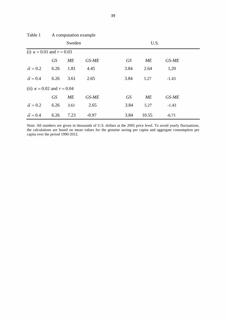
39

Table 1 A computation example

Sweden U.S.

(i) 0.01 and 0.03rκ = =

GS ME GS-ME GS ME GS-ME

0.2α = 6.26 1.81 4.45 3.84 2.64 1,20

0.4α = 6.26 3.61 2.65 3.84 5.27 -1.43

(ii) 0.02 and 0.04rκ = =

GS ME GS-ME GS ME GS-ME

0.2α = 6.26 3.61 2.65 3.84 5.27 -1.43

0.4α = 6.26 7.23 -0.97 3.84 10.55 -6.71

Note: All numbers are given in thousands of U.S. dollars at the 2005 price level. To avoid yearly fluctuations, the calculations are based on mean values for the genuine saving per capita and aggregate consumption per capita over the period 1990-2012.

Documents

Genuine Saving and Conspicuous Consumption · (2010), and Corazzini, Esposito, and Majorano (2012). See also Fliessbach et al. (2007) and Dohmen et al