Wind induced variability in the Northern Current (North-WesternMediterranean Sea) as depicted by a multi-platform observingsystemMaristella Berta1, Lucio Bellomo2,3, Annalisa Griffa1,4, Marcello Magaldi1,5, Anne Molcard2,3,Carlo Mantovani1, Gian Pietro Gasparini1, Julien Marmain6, Anna Vetrano1, Laurent Béguery7,Mireno Borghini1, Yves Barbin8, Joel Gaggelli8, and Céline Quentin8
1CNR-ISMAR, Lerici, Italy2MIO, Université de Toulon, CNRS, IRD, La Garde, France3MIO, Aix-Marseille Université, CNRS, IRD, Marseille, France4RSMAS, University of Miami, Miami, FL, USA5Johns Hopkins University, Baltimore, MD, USA6Degreane Horizon, Cuers, France7ACSA, 9 Europarc, 13590 Meyreuil, France8MIO, CNRS, Aix-Marseille Université, Université de Toulon, IRD, Marseille, France
Correspondence: Maristella Berta ([email protected])
Abstract. The variability and evolution of the Northern Current (NC) in the area off Toulon is studied for two weeks in
December 2011 using data from a glider, a HF radar network, vessel surveys, a meteo station, and an atmospheric model. The
NC variability is dominated by a synoptic response to wind events, even though a seasonal trend is also observed, transitioning
from late summer to fall-winter conditions. With weak winds the current is mostly zonal and in geostrophic balance even at
the surface, with a zonal transport associated to the NC of ≈ 1 Sv. Strong westerly wind events (longer than 2-3 days) induce5
an interplay between the direct wind induced ageostrophic response and the geostrophic component: upwelling is observed,
with offshore surface transport, surface cooling, flattening of the isopycnals and reduced zonal geostrophic transport (0.5-0.7
Sv). The sea surface response to wind events, as observed by the HF radar, shows total currents rotated at ≈−55◦ to −90◦ to
the right of the wind. Performing a decomposition between geostrophic and ageostrophic components of the surface currents,
the wind driven ageostrophic component is found to rotate of ≈−25◦ to −30◦ to the right of the wind. The ageostrophic10
component magnitude corresponds to ≈ 2% of the wind speed.
1
Ocean Sci. Discuss., https://doi.org/10.5194/os-2018-20Manuscript under review for journal Ocean Sci.Discussion started: 1 March 2018c© Author(s) 2018. CC BY 4.0 License.
1 Introduction
The Liguro-Provenço-Catalan Current, also called Northern Current (Millot, 1999), is a boundary current corresponding to the
upper limb of the Western Mediterranean circulation (Fig.1a). It originates in the Ligurian Sea due to the convergence of the
two currents flowing along each side of the Corsica island (Astraldi and Gasparini, 1992), namely the Western and Eastern
Corsica Currents (WCC and ECC). The Northern Current (denoted NC hereafter) flows southwestward along the continental5
slope of the Ligurian-Provençal and Balearic basins with a certain degree of continuity and may thus be recognized as a single
entity as far as the Catalan Sea (Millot, 1987; Font et al., 1988; Garcia et al., 1994). Its importance mainly relies on the fact
that all water masses in the area - namely the Modified Atlantic Water (MAW), the Levantine Intermediate Water (LIW) and
the Western Mediterranean Deep Water (WMDW) - are carried by the current during its flowing (Conan and Millot, 1995). As
a result, the NC is known to influence the coastal circulation of the Gulf of Lion (Duchez et al., 2012) and most importantly,10
to modulate the supply of salt and/or heat by lateral advection in the convection areas (the so called preconditioning, see
Schroeder et al. (2010)) and thus affect the important deep water formation process in the Western Mediterranean. Also, the
NC hugs the highly populated coasts of Italy and France, where areas of intense industrial development alternate with turistical
and environmental relevant Marine Protected Areas (MPAs). Understanding the flow dynamics and how it carries biological
and pollutant quantities is of great importance for a correct management of coastal and marine activities.15
The NC has been intensively observed in a few specific places of the southern French coast, namely a) off Nice (Béthoux
et al., 1982; Taupier-Letage and Millot, 1986; Béthoux et al., 1988; Albérola et al., 1995a; Sammari et al., 1995); b) at the
eastern edge of the Gulf of Lion, off Marseilles (Conan and Millot, 1995; Flexas et al., 2002; Albérola and Millot, 2003;
Forget et al., 2008) and c) along the Gulf of Lion shelf break (Lapouyade and de Madron, 2001; Petrenko, 2003; André et al.,
2009; Rubio et al., 2009). All this past literature agrees on some of its large scale characteristics: the NC is confined within20
approximately 35−40 km from the coast and has an average geostrophic transport value of about 1.8 Sv (1 Sv = 106 m3 s−1)
(Béthoux et al., 1982; Sammari et al., 1995). It exhibits a marked annual cycle: during winter it gets stronger, closer to coast,
narrowing (about 25 km) and deepening (about 450 m), while in summer, it weakens, extends more offshore increasing its
width around 40 km, and gets thinner (about 250 m). Mesoscale activity also increases from late autumn to winter and then it
decreases in summer, and it is concentrated in two main time windows of 3-6 days and 10-20 days respectively (Taupier-Letage25
and Millot, 1986; Millot, 1987; Albérola et al., 1995a; Sammari et al., 1995).
Despite the numerous articles above, the study of the NC and its variability still represents an active area of research,
especially at scales shorter than seasonal. Transport measurements provide a wide range of values in the literature, reaching
minimum values of 0.5 Sverdrup and showing significant variability in time (Conan and Millot, 1995) and in space (Petrenko,
2003). The reason for this variability within the annual cycle is not clear yet. It has been suggested that it may be due to different30
freshwater signals from precipitation and river runoff (Béthoux et al., 1988), to the WMDW formation process (Crépon and
Boukthir, 1987), or inherited by the distinct behavior of the WCC and the ECC, whose annual peaks differ of several months
(Astraldi and Gasparini, 1992).
2
Ocean Sci. Discuss., https://doi.org/10.5194/os-2018-20Manuscript under review for journal Ocean Sci.Discussion started: 1 March 2018c© Author(s) 2018. CC BY 4.0 License.
In particular, the study of variability of the NC in the area off Toulon (between Nice and Marseilles) deserves particular
attention for various reasons. The NC dynamics has been undersampled in the past and far less documented than in other regions
such as off Nice and Marseille. Only recently the NC mesoscale meandering off Toulon has been specifically investigated
through the comparison of models and observations (Guihou et al., 2013) and with data assimilation (Marmain et al., 2014).
These studies indicate the role of prevailing northwesterly winds in the modulation of the NC circulation. In fact, the area near5
Toulon is peculiar because the mean NC circulation is resisted by the prevailing northwesterly winds in the area. The upwelling
prone winds can significantly alter the current, to the point that in some occasions they can stop its westward propagation and
control its penetration in the Gulf of Lion (Millot and Wald, 1980). When this happens, a frontal zone separating warm NC
waters and cold waters upwelled from the Gulf of Lion is established near the coast, and it has clearly been observed from
satellite images (Millot and Wald, 1980).10
In this paper, the variability of the NC in the area off Toulon is studied using results from a multi-platform experiment
involving HF radar, glider, a meteo station, and a research vessel, carried out in the framework of the EU-MED project TOSCA
(Tracking Oil Spills and Coastal Awareness network, http://www.tosca-med.eu). The experiment took place during a period
of approximately two weeks in December 2011 (December 2-19), characterized by intense westerly and northwesterly wind
events. The wind response of coastal boundary currents such as the NC is complex, and based on the interplay between the15
direct ageostrophic response in the surface layers and the geostrophic modifications occurring along the whole water column.
The response of boundary currents to winds has been studied by several authors using numerical model results, satellite and
in-situ data (Magaldi et al., 2010; Aguiar et al., 2014; Schaeffer and Roughan, 2015). Experimental works are mostly based on
a statistical approach, i.e. using long time series of wind and currents and computing correlations or identifying the main flow
patterns corresponding to specific wind forcing (Kosro, 2005; Kim et al., 2010; Mihanovic et al., 2011; Yuan et al., 2017).20
Here, we focus on the dynamics of specific wind events, and take advantage of the multi-platform information, especially
from HF radars for the surface and glider for the water column. Our general goal is to identify the main processes at work, and
to investigate how to unravel the interplay between the direct wind induced surface response and the geostrophic response. The
following two specific goals are pursued:
1) to describe the sea current system evolution during the period of interest, quantifying the water column response to the25
wind in terms of isopycnal and zonal geostrophic velocity evolution;
2) to investigate the surface layer response to the wind, attempting a decomposition between geostrophic and ageostrophic
components of the velocity.
The problem of decomposing the surface flow in geostrophic and ageostrophic components has been previously addressed
in several works. Earlier works used hydrographic or ADCP information to infer the geostrophic flow (e.g. Weller et al. (1991);30
Chereskin and Roemmich (1991); Wijffels et al. (1994)), while more recently the global altimetric products (Lagerloef et al.,
1999) have been used in several applications. Rio and Hernandez (2003) used SVP drifters and altimetry to infer information at
global scales, while HF radar results with altimetry have been used to compute wind driven velocities in the Kuroshio Current
(Tokeshi et al., 2007) and in the South Atlantic Bight (Yuan et al., 2017). For coastal boundary currents such as the NC and for
the space and time scales we are interested in, though, the use of altimeter is not appropriate. In this paper, we investigate the35
3
Ocean Sci. Discuss., https://doi.org/10.5194/os-2018-20Manuscript under review for journal Ocean Sci.Discussion started: 1 March 2018c© Author(s) 2018. CC BY 4.0 License.

use of glider data in conjunction with HF radar. There are several challenges in using glider transects, including limited space
and time sampling (Piterbarg et al., 2014) and the fact that only one component of the geostrophic velocity can be retrieved.
Here we investigate how to best combine glider and HF radar data and in which flow conditions they can be best exploited.
The paper is organized as follows. In Section 2, the main questions addressed in the paper are stated, and the main definitions
are introduced. In Section 3, a description of the data as well as the methods used to analyze them is provided. In Section 4,5
a description of the sea current system evolution over the whole water column is provided, while the analysis of the wind
response in the surface layer is performed in Section 5. A summary and discussion are provided in Section 6.
2 Background, statement of the problem and definitions
As stated in the Introduction, the general goal of this work is to investigate the variability of the NC during the period of interest,
with special focus on the response of the system to wind forcing, using information from glider and HF radar. The velocity10
field of the system u(x,y,z, t) can always be written through kinematic decomposition as the superposition of a geostrophic
and an ageostrophic component:
u = ug + ua (1)
The geostrophic part ug obeys to the balance between pressure gradient and earth rotation (Coriolis). In the case of a
boundary current, ug is expected to be driven by the large scale pressure gradient of the general circulation, as well as by the15
more localized pressure gradient of mesoscale phenomena such as meanders and eddies (Centurioni et al., 2008; Gangopadhyay
et al., 2013). The ageostrophic component, ua includes the phenomena that are not in geostrophic balance. In the water column
interior, we can expect that the flow is mostly geostrophic at scales longer than a day, while high frequency processes such as
internal waves, tides or inertial oscillations, play an important role at shorter time scales (Mensa et al., 2013).
At the surface, in addition to high frequency processes, also ageostrophic processes related to direct wind and air-sea inter-20
action are relevant. In particular, the surface velocity, uS(x,y, t) can be written as:
uS = uSg + uSaW + uSR (2)
where uSg is the surface geostrophic velocity, uSaW is the directly wind driven component, and uSR includes all the other
high frequency processes such as tides, inertial and submesoscale variability, that for the purpose of this paper we will refer to
as “residual”.25
The wind response uSaW has been studied for many decades, starting from the pioneering work by Ekman (1905), con-
sidering idealized solutions of the balance between Coriolis and friction. The classic Ekman solution, valid in stationary and
homogeneous conditions of infinite domain in the horizontal and at depth, is characterized by a surface current at 45◦ to the
right of the wind (in the Northern hemisphere) spiraling with depth in the surface layer. The solution is highly dependent
4
Ocean Sci. Discuss., https://doi.org/10.5194/os-2018-20Manuscript under review for journal Ocean Sci.Discussion started: 1 March 2018c© Author(s) 2018. CC BY 4.0 License.
on the specific parameterization of wind stress and vertical diffusivity. As an example, assuming that the wind stress linearly
decreases with depth, leads to the “slab” solution, which is 90◦ to the right of the wind and constant with depth (Pollard and
Millard, 1970). The choice of other parameterizations as well as the presence of boundaries, finite depth, time dependence
and inhomogeneity further modifies the solution (Endoh and Nitta, 1971; Ralph and Niiler, 1999; Crise et al., 2006). Also, it
can be expected that the simplified balance of the Ekman equation only partially captures the dynamics in realistic conditions,5
because of the interactions between the various processes. Indeed, direct measurements show a great range of variability in the
observed wind response (Rio and Hernandez, 2003; Sentchev et al., 2017). In summary, even though the idealized solutions
provide very important general guidance, the actual surface response to the wind in realistic conditions is still an open question
(Stanichny et al., 2016), and it can be expected to depend on the specific environmental conditions.
We notice that there is a well known direct dynamical link between uSaW and the geostrophic velocity ug . In the case of10
a boundary current, when the wind induces cross-shore transport, the cross-shore pressure gradient can be modified provided
that the wind acts for a sufficiently long time scale, TW (Whitney and Garvine, 2005). For the Northern Current, Piterbarg
et al. (2014) estimated that for winds of the order of 10 ms−1 TW is of the order of 2.5 - 3 days. In the case of upwelling prone
winds, as is the case of the westerly winds considered here, the ageostrophic surface response causes offshore transport that is
compensated by deep water coastal upwelling, modifying both the surface pressure gradient and the water column stratification15
estimated by the potential density anomaly σ(z). This in turns, alters the along-shore geostrophic component of the flow. In
addition to this main mechanism, the geostrophic response can be further modulated by several other mechanisms, such as
nonlinear frontal wind response (Oguz et al., 2017), and interactions with mesoscale and submesoscale instabilities.
The work performed here has two specific goals:
1) Describe the variability of the NC over the whole water column and investigate its relationship with wind forcing.20
The full 3D description of u(x,y,z, t) is clearly not available from our data, but the data from glider and HF radar provide
a good first approximation of the sea current system. The radar data provide estimates of the 2-D surface velocities u(x,y, t),
while the glider data provide information on the interior flow in terms of stratification, σ(y,z, t), and zonal geostrophic velocity,
ug(y,z, t), estimated along the cross-shore glider transect. In this part of the work, we concentrate on variability over time scales
of one day or longer, in keeping with the use of glider transect data and geostrophic velocities. In particular, we investigate the25
response of the sea current system during intense westerly wind events and concentrate on the main mechanism between wind
induced surface transport and upwelling response. Other mechanisms such as nonlinear wind response and interaction with
instabilities are not directly considered here because we do not have enough information to resolve the various aspects.
2) Further investigate the wind response in the surface layer and test a method to estimate the induced ageostrophic compo-
nent uSaW .30
The high frequency response of the surface velocity uS(x,y, t) as provided by the radar is used as a basis for the analysis.
The estimate of uSaW is performed during periods of high winds, when it can be assumed that this term is prevalent with
respect to uSR in eq. (2). Still, the difficulty lies in identifying a reliable estimate for uSg(x.y.t) to be subtracted to uS(x,y, t)
in eq. (2). A simple method based on the combined analysis of glider and HF radar data is put forth, valid for specific dynamic
regimes.35
5
Ocean Sci. Discuss., https://doi.org/10.5194/os-2018-20Manuscript under review for journal Ocean Sci.Discussion started: 1 March 2018c© Author(s) 2018. CC BY 4.0 License.
3 Data and methods
Here we review the data sets used in this study and describe the main data treatments and analyses that have been carried out.
The data spatial coverage is shown in Fig.1b, while a time line of the measurements is shown in Fig.2a
3.1 Vessel based measurements
During the experimental effort, an oceanographic cruise took place aboard the Italian R/V Urania between December 10 and5
15, 2011. While measurements were performed within an extended offshore area between Nice and Toulon, here we consider
only the Toulon measurements taken on December 13 and 14. A total of 11 CTD stations were sampled in the surrounding of
the glider transect (Fig.1b). The CTD data have been used for intercomparison and calibration of the glider hydrographic data
as further discussed in Sections 3.2-3.3.
3.2 Gliders10
An autonomous underwater glider of the Slocum kind (Jones et al., 2005), manufactured by Webb Research Corporation, has
been deployed and maintained operational during the period December 2-19 (Fig. 2a). The glider, named Hannon, covered 6
repeated meridional transects off Toulon extending ∼70 km offshore (Fig. 1b). The onshore half of the transects laid within
the HF radar coverage. The maximum profiling depth was set to 1000 m, giving mean horizontal distance between consecutive
profiles, mean horizontal speed, and mean vertical speed of 1.7 km, 35 cms−1, and 20 cms−1, respectively. The timing details15
of each transect are summarized in the timeline in Fig.2a and in Table 1.
Hannon was equipped with an unpumped SBE 41 CTD manufactured by Sea-Bird Electronics. CTD data were processed
with dedicated Matlab routines taking care of all classic CTD response times and alignment issues, and all parameters were
rebinned onto a regular vertical grid with a step of 2 dbar. Due to the use of an unpumped CTD and to the variable speed of the
autonomous vehicle, the corrections were made speed-dependent using the glider speed computed through pressure variations20
and tilt angle. The thermal lag of the conductivity sensor was dealt also with speed-dependent coefficients (Morison et al.,
1994) experimentally found through the technique proposed by Garau et al. (2011). The optimum values of the coefficients
were αo = 0.5447, αs = 0.0708, τo = 9.5117, and τs = 7.69. Finally, temperature and conductivity values were post-calibrated
against the Sea-Bird Electronics SBE 911+ CTD deployed from the R/V. For this purpose, only glider and ship profiles distant
less than 14 km and separated by less than 12 h were considered, discarding all data shallower than 600 dbar.25
3.3 Glider data analyses: isopycnal structure and computation of zonal geostrophic velocities
The glider hydrographic data were used to describe the NC current stratification and evolution. The hydrographic glider data
have also been used to compute relative geostrophic velocities in the direction perpendicular to the glider transects, corre-
sponding to the zonal direction. Potential density profiles were used, previously low-pass filtered through a Gaussian filter
with 9-km cut-off wavelength (Rossby radius found through the dynamic mode decomposition of the average Brunt-Väisäla30
frequency profiles (Kundu et al., 1975). Although depth-averaged velocities from the glider could have been used to reference
6
Ocean Sci. Discuss., https://doi.org/10.5194/os-2018-20Manuscript under review for journal Ocean Sci.Discussion started: 1 March 2018c© Author(s) 2018. CC BY 4.0 License.

the geostrophic velocities (as done e.g. by Davis et al. (2008)), a calibration problem in Hannon magnetic compass prevented
us from doing so. Therefore, the velocities were referenced to a level of no motion z0, assumed to be in the range between
500-700 m. Sensitivity tests on z0 between 500 and 700 show very limited variability, with root mean square differences in the
mean upper layer velocity of ≈ 2%. In the following, results with z0= 500 m are used.
The zonal geostrophic velocities were used also to compute the integrated transport, using the 5 cms−1 isotach to identify5
the Northern Current, as done e.g. by Albérola et al. (1995a) and Conan and Millot (1995).
3.4 HF radar
The HF radar system has been operational during the period December 6-19 (Fig. 2a), covering the area in front of Toulon
(Fig. 1b). The HF radar installation is based on the WERA technology (Gurgel et al., 1999) and relies on two systems. The first
one (Fort Peyras, “FP” in Fig. 1b) has a quasi-monostatic configuration with an irregular, W-shaped 8-antenna receiving array10
and 2 monopoles performing the emission while forming a zero in the direction of the receiver. The peculiarity of the receiving
array geometry is imposed by the environment of the site, a dismissed military base. The second system (Cap Bénat, “CB” in
Fig. 1b) has a fully bistatic configuration, with the 2 monopoles in FP employed as emitter, and a regular linear 8-antenna array
in CB operated as receiver (transmitter and receiver are 35 km apart).
The two systems operate at a frequency of 16.1 MHz with 50 kHz bandwidth, giving a nominal range resolution in the radial15
direction of 3 km. Antenna patterns are routinely measured almost every year and they had been applied to the December 2011
data set. The azimuthal processing is done with the MUSIC (MUltiple SIgnal Characterization) direction finding algorithm
with a nominal 2 deg spacing (Lipa et al., 2006; Molcard et al., 2009; Sentchev et al., 2013), and radial velocity maps are
produced every 20 min by integrating over the previous hour. Total velocity maps are then obtained on a regular 2 km grid
through a local interpolation method which, at each grid point, minimizes the Mean Square Error (MSE) between the projection20
of the total velocity onto the radial directions and the radial velocities available within a 3 km-radius circle (Lipa and Barrick,
1983). Classically, total velocities are only computed when the angle between radial data from the two systems lies within the
range 30− 150◦, which corresponds to GDOP values smaller than 2.5 (Chapman et al., 1997).
In our case, the requirement on the angle had to be reduced to 20− 160◦ (corresponding approximately to GDOP values
smaller than 4) in order to keep an acceptable offshore coverage on the region for the bistatic configuration. The Toulon radar25
system has been validated also during other TOSCA experiments involving the deployment of drifters, used to compare HF
radar fields and derived velocities from in situ trajectories. Results show a high level of accuracy, on average 80% agreement
between drifters and HF radar, consistently using FP as quasi-monostatic configuration, CB as a different bistatic configuration
(with the emitter in Porquerolles transmitter and receiver are 16 km apart) and GDOP values smaller than 2.5 (Berta et al.,
2014; Bellomo et al., 2015).30
HF radar measured velocities are the results of a vertical integration, through an exponential weighting function, over a
characteristic depth λ0/4π (Stewart and Joy, 1974), where λ0 is the resonant Bragg wavelength, which is half the wavelength
of the emitted electromagnetic wave. For our systems, operating at a central frequency of 16.1 MHz,the characteristic depth is
about 75 cm.
7
Ocean Sci. Discuss., https://doi.org/10.5194/os-2018-20Manuscript under review for journal Ocean Sci.Discussion started: 1 March 2018c© Author(s) 2018. CC BY 4.0 License.

Due to the proximity of the FP site emitter with respect to the receiver array, imposed once again by the constraints of the
military base, the HF radar coverage systematically experienced a drastic loss under strong Mistral winds. In fact, the wind-
induced vibrations of the emitter antennas generated a phase noise in the receiver antennas frequency spectrum, making in turn
the signal-to-noise ratio unacceptably low at usually well-covered distances. Unfortunately, the problem was solved only after
the observational campaign by placing the emitter farther outside the military base.5
3.5 Analysis and interpretation of HF radar data
The HF radar fields are used to describe the evolution of the surface velocities. Preliminary tests have been performed using
the raw data as well as low pass filtered data with a cut-off period of 36 h. Results, using raw and filtered data, agree within
86% to 99% in terms of average and rms velocites for v and u component respectively, so that only results based on raw data
are presented in the following.10
We point out an important general issue regarding the interpretation of results based on HF radar velocities. Several papers
(Mao and Heron, 2008; Ardhuin et al., 2009) have pointed out that the HF radar based surface velocity has, in addition to
the actual Eulerian velocity u(x,y, t), also a nonlinear wave correction (Weber and Barrick, 1977) that can be interpreted as a
filtered surface Stokes drift, including the contribution of waves with wavelengths longer than the Bragg resonant wavelength.
A method to estimate this term has been proposed based on an accurate numerical wave model (Ardhuin et al., 2009). A15
debate is ongoing in the literature regarding the magnitude of the term and whether is significant or not (Mao and Heron, 2008;
Röhrs et al., 2015). An important factor is the fetch, since the longer is the fetch the more important is the contribution of long
waves (Essen et al., 2000). In our case, the Bragg resonant wavelength for our system is approximately 9 m, and the Stokes-like
term cannot be explicitly estimated following Ardhuin et al. (2009) because we do not have access to the full wave spectrum
information for the period of interest. Since the wind is predominantly from the west and north-west and given the geography20
of the region (Fig.1a), we can expect that the fetch is limited and therefore the term is unlikely to be relevant. In absence of a
quantitative estimate, though, we caution that the wind response term uSaW for our measurement could include not only the
Ekman-type Eulerian response, but also a possible Lagrangian contribution from Stokes drift. We will come back to this point
in Section 5.
3.6 Wind data from meteo station and model25
Hourly wind speed and direction measurements have been provided for the complete period of 2-19 December by the Me-
teoFrance’s Porquerolles meteo station whose location is shown in Fig.1b. In addition, Meteo France’s ALADIN operational
regional model (1/10◦ and 3 h space and time resolution, respectively) has also been used.
Time series of wind speed and directions from the meteo station and from the model averaged over the area of interest
(Fig.1b) are shown in Fig.2b. The results are qualitatively very similar, showing the good agreement of the model with the data30
and indicating that the wind patterns in the area are not characterized by strong gradients during the period of interest. Only
during the last few days, after December 18, the two time series show significant differences.
8
Ocean Sci. Discuss., https://doi.org/10.5194/os-2018-20Manuscript under review for journal Ocean Sci.Discussion started: 1 March 2018c© Author(s) 2018. CC BY 4.0 License.

From the wind time series, events of high wind speed have been identified, considering a threshold of 10 ms−1. This choice
is consistent with the Beaufort scale (www.spc.noaa.gov), and it is confirmed a-posteriori by the consistency of the results as
discussed in Section 5. As shown in Fig.2a,b, the period of interest is characterized by two main events that last more than
3 days, E1 and E3, and a shorter event lasting less than 1 day, E2. The main wind direction is westerly and northwesterly,
compatible with Mistral events in the area. We notice that, E1 and E3 have duration longer than the estimated value of TW5
in the area (2-3 days), and therefore are likely to influence stratification and geostrophic velocity in the NC, as discussed in
Section 2. The opposite holds for E2.
3.7 Summary of the measurements
In summary, the time line of the main measurements carried out during the experiment is provided in Fig. 2a and includes:
– Glider measurements (red boxes). They cover the period December 2-19 for a total of 6 transects, alternating offshore10
and inshore routes.
– HF radar measurements (solid gray). They start December 6, so that the first glider transect does not have contemporary
HF radar data. The periods in which the glider transects fall inside the radar coverage are shown by green dashed lines.
– Wind measurements and model outputs. They are available during the whole period December 2-19. The three wind
events E1, E2, and E3 are shown as dashed black lines.15
4 Water column stratification and geostrophic variability, and effects of wind forcing
In the following, the variability of the Northern Current is described during the period of interest December 2-19. For simplicity
we partition the time of the analyses following the same time intervals as for the glider transects (Table 1, Fig.2a). For each
transect period, we provide a basic description based on the wind evolution together with the glider results on hydrography and
zonal geostrophic velocity, and (when available) on the time-averaged surface velocity fields from HF radar. Radar velocity20
field averages are computed during periods in which the glider transects fall inside the radar coverage and considering only grid
points with more than 80% measurement coverage in time, in order to avoid mean flow contamination due to inhomogeneous
coverages. For selected transects, all the information above from glider and HF radar are shown grouped together in a single
multi-panel figure (Figs. 3-6).
In order to quantify the flow variability we show also some comprehensive figures that compare all transects in terms of25
the following metrics: evolution of the isopycnals σ(z) (Fig.7), zonal geostrophic transport (Fig.8), and comparison between
surface zonal geostrophic velocity uSg estimated from the glider data and total surface velocity uS considering HF radar data
along the glider tracks (Fig.9).
9
Ocean Sci. Discuss., https://doi.org/10.5194/os-2018-20Manuscript under review for journal Ocean Sci.Discussion started: 1 March 2018c© Author(s) 2018. CC BY 4.0 License.

4.1 Transect 1 : initially calm condition followed by the onset of wind event E1
During Transect 1 (December 2-4) the glider moves offshore from the coast, and no HF radar are available (see Fig.2a). The
wind speed (Fig.2b) is initially weak, and then the first westerly event E1 starts on December 3. Notice that the period before
the experiment (not shown) was characterized by calm conditions, with a week of weak winds, with speed smaller than 7.5
ms−1.5
The hydrographic properties (potential temperature θ and practical salinity S) of Transect 1 are shown in panels a,b of Fig.3
for the first 300 m, with overlying isolines of potential density anomaly σ(z). The transect plot origin of all hydrographic
panels shown in the following figures is located a few kilometers off the coast (starting point of the glider mission). Following
Boucher et al. (1987), we refer to the three zones that can be typically distinguished in the NC structure on the basis of the
shape of the isopycnals with potential density anomaly σ in the range 28.7 - 29.05 kgm−3: the inshore flat part of the isopycnals10
defines the “coastal” (or marginal) zone, the sloping part identifies the “frontal” zone where the NC is most energetic, and the
flat offshore part denotes the “central” basin zone. Here, we use σ=28.7 kgm−3 to characterize these zones (see also Fig. 7).
The coastal marginal zone (typically flat) is not visible in the glider transect, while the frontal zone is evident and it extends
up to ≈ 42.5◦ N, i.e. at ≈ 40-45 km offshore. The θ and S transects (Fig. 3a,b) show a strong thermocline at 50 m in the
offshore central region, accompanied by the presence of a salinity minimum right below it in the frontal zone. These conditions15
are typical of late summer conditions (Guibout (1987) pp. 16 and 18 off Toulon and p. 36 off Nice), that apparently are still
present at the beginning of the experiment. The zonal geostrophic velocity ug computed along the transect shows a westward
current extending up to 60 km off the coast with core (up to 0.4ms−1 in first 100m) located at ∼42.7◦-42.8◦ (Fig.3c). The
offshore limit and depth of the NC are approximately ∼ 55 km and ∼175 m, respectively, with the core situated roughly at km
25 (Albérola et al., 1995a; Petrenko, 2003). The relatively large width and shallowness of the observed current here, known to20
be narrower and deeper than this during winter Albérola et al. (1995a), confirm the presence of late-summer conditions at the
beginning of the experiment.
4.2 Transect 2-3 : Wind event E1
During the following two Transects, 2 and 3, (December 4-7 and 7-9 respectively) while the glider travels back inshore and
then offshore again, the wind is mostly dominated by the westerly event E1 (Fig.2b), tapering off toward the end of the period.25
HF radar data are available starting from December 6 (Fig.2a). The results of the two transects are qualitatively similar, so the
complete results are shown only for Transect 3 in Fig.4.
The hydrographic transects from the glider show a significant change with respect to Transect 1 (Fig.3). Surface waters
in the frontal zone are colder of ≈ 1.5◦C and the shape of the isopycnals is significantly flattened, while the mixed layer in
the offshore central part is deepened of ≈ 20-30 m. This can be seen clearly also in Fig.7, where the isopycnal with σ = 28.730
kgm−3 for all transects are shown. Transects 2 and 3 show very similar isopycnal shape in the frontal area, flatter and shallower
than for Transect 1. In the offshore central region, on the other hand, the isopycnal of Transect 2 is similar to the one of Transect
1, while for Transect 3 it deepens of ≈ 20-30 m. This is likely due to the different sampling times, since the glider covers the
10
Ocean Sci. Discuss., https://doi.org/10.5194/os-2018-20Manuscript under review for journal Ocean Sci.Discussion started: 1 March 2018c© Author(s) 2018. CC BY 4.0 License.

offshore region in Transect 3 about two days later than for Transect 2, and Transect 2 itself takes place shortly after the onset
of E1 wind event (Fig.2a).
The average surface velocity uS depicted by the HF radar during the glider sampling (Fig.2a) is shown in Fig.4d. Notice the
reduced coverage with respect to the expected coverage (Fig.1b), due to wind induced interferences as discussed in Section 3.4.
The velocity shows an overall offshore transport, with localized eastward reversals of the zonal current in the north western5
part of the radar coverage. The prevalent offshore current is consistent with the expected wind driven transport to the right of
the prevalent westerly wind (more in depth discussion is provided in Section 5).
Overall, the results suggest the presence of an upwelling phenomenon associated to the offshore transport induced by the
westerly winds, that causes the flattening of the isopycnals in the frontal region and the cooling at the sea surface. In addition to
the upwelling, other phenomena related to wind response are likely to occur, as suggested by the offshore isopycnal deepening10
in Figs.4 and 7, likely due to mixing that deepens the thermocline and possibly to convection processes.
The zonal geostrophic velocity ug(y,z) computed from the glider (Fig.4c) is mostly westward but reduced with respect to
Transect 1 (T1) in Fig.3c, as expected during an upwelling episode. The difference between geostrophic velocity in T1 and T3,
considering also the elapsed time between the two transects, is consistent with the estimate of the time scale TW (Whitney and
Garvine, 2005) of 2-3 days needed for wind events to affect geostrophy in the NC (Piterbarg et al., 2014), and it suggests that15
E1 can modify stratification and geostrophic velocity after a sufficiently long wind forcing period.
The change in ug(y,z) is quantified computing the corresponding zonal transport (Fig.8). For the integrated transport com-
putation the 5 cms−1 isotach was used to identify the Northern Current, as done e.g. by Albérola et al. (1995a) and Conan and
Millot (1995). A very strong variability is seen with respect to the first transect, with the transport reduced of ≈ 50% going
from ≈ 1.15 Sv for T1 to 0.7-0.6 Sv for T2 and T3.20
Finally, we provide a preliminary assessment of the surface deviation from geostrophy (that will be further investigated in
Section 5) by comparing the magnitude of the zonal geostrophic velocity uSg from the glider with the total velocity uS depicted
by the radar along the glider track (Fig.9). During T2, the zonal radar total velocity is significantly lower than the geostrophic
one, while the meridional component of the total velocity is almost the double of the zonal one. Results for T3 are qualitatively
similar but incomplete because of the limited radar coverage. The observed magnitude difference in the zonal component from25
glider (geostrophic) and radar (total velocity) suggests that ageostrophic processes play a non negligible role at the sea surface
for T2-T3.
4.3 Transects 4-5 : calm conditions interrupted by wind event E2 and onset of E3
The following two transects, T4 and T5, (December 9-12, 12-15 respectively) are characterized by mostly calm wind conditions
(Fig.2a), except for the brief westerly wind event E2, occurring in between the two transects. Winds during the calm period30
are mostly westerly, except for some strong direction oscillations prevalent for lowest wind speed (below 4-5ms−1), mostly
evident in the Porquerolles station records. During the last day of T5, the onset of the third wind event E3 occurs. Notice that
E2 lasts less than a day, which is significantly less than TW estimetad by Piterbarg et al. (2014), so that it is not expected to
11
Ocean Sci. Discuss., https://doi.org/10.5194/os-2018-20Manuscript under review for journal Ocean Sci.Discussion started: 1 March 2018c© Author(s) 2018. CC BY 4.0 License.

modify the stratification and geostrophic velocity, structure even though of course it influences surface velocity. The results of
T4 and T5 are qualitatively similar, and the T5 results are shown in Fig.5
The hydrographic transects (Fig.5a,b) indicate a narrowing and steepening of the frontal region characterized by warmer
and fresher water in the surface layer. This is shown also by the σ isopycnals in Fig.7 that are very similar for T4 and T5, and
suggests a strong frontal area closer to the coast, approximately north of 42.7◦ N.5
The zonal geostrophic velocity uSg (Fig.5c) indeed shows a narrower but deeper and intensified current. The corresponding
zonal geostrophic transport (Fig.8) increases with respect to T2-T3, reaching values of ≈ 1− 0.9 Sv for T4 and T5.
The radar surface velocity (Fig.5d) is very different from the previous transects (Fig.4d). The coverage is more extended
and the velocity is almost completely zonal, showing the typical westward structure of the Northern Current. Notice that, even
though the current actually deviate from the zonal direction during E2 (as further discussed in Section 5), the contribution to10
the average shown in Fig.5d is very modest, because the average is performed during the glider sampling that overlaps only
for a few hours with E2 (Fig.2a). Also, E2 does not appear to modify significantly the stratification, the geostrophic velocity
and the associated transport, as it can be seen by the comparison of the two transects T4 and T5 in Figs. 7-8. This is in keeping
with the fact that the duration of E2 is shorter than TW .
The surface comparison between geostrophic uSg and total velocity uS from HF radar shows an excellent agreement in the15
zonal direction for both T4 and T5 (Fig.9c,d), while the meridional component in the frontal region is significantly lower than
the zonal one (approximately 70% and 85% for T4 and T5 respectively). Overall, the results suggest that the current during
these two transects is mostly zonal and geostrophic even at the surface, i.e. sustained by the large scale pressure gradient that
maintain the general and mesoscale circulation in the Ligurian basin.
4.4 Transects 6: wind event E320
The last transect T6 (December 15-18) is dominated by the wind event E3, that is mostly westerly but veering toward northerly
during the last day. The results are summarized in Fig.6.
The hydrographic transects show a cooling of ≈ 1-1.5◦C in the frontal region, together with a strong flattening of the
isopycnals as shown also in Fig.7. The surface velocity depicted by the HF radar (Fig.6d) is mostly meridional and offshore,
in agreement with a wind response leading to upwelling. The geostrophic velocity is reduced (Fig.6c), and the westward jet25
structure appears fragmented. The corresponding zonal geostrophic transport is reduced with respect to the previous transects,
and is even lower than for T3 and T4, reaching values of ≈ 0.45 Sv (Fig.8). The comparison between surface geostrophic uSg
and radar based total velocity uS (Fig. 9e) shows a significant deviation from geostrophy at the surface, as expected. uSg has
a complex pattern, while uS is dominated by the meridional component (≈ 30% bigger than the zonal velocities).
Overall, the results are qualitatively similar to the ones of T2 and T3, describing an upwelling response to the wind that30
influences and weakens the geostrophic circulation. It is interesting to notice, though, that there are also some differences in
the hydrographic properties with respect to the previous transects that are likely to be related to the transition from late-summer
to winter conditions. The salinity minimum present in the first transect (Fig. 3b) vanishes with time and it is almost absent in
T6 (Fig. 6b), suggesting that the late summer conditions in T1 are turning toward a more typical winter configuration, probably
12
Ocean Sci. Discuss., https://doi.org/10.5194/os-2018-20Manuscript under review for journal Ocean Sci.Discussion started: 1 March 2018c© Author(s) 2018. CC BY 4.0 License.

due to the recurring effects of upwelling and mixing associated with the winter wind episodes. This is also shown by the
pycnocline deepening of ≈ 30 m in the offshore central region (Fig.7), occurring after the first two glider transects.
4.5 Summary of results
The main results from the above analysis can be summarized as follows.
– The observed variability of the Northern Current during the experiment period is dominated by wind response. In addition5
to this synoptic variability, the overall hydrographic conditions also suggest a seasonal trend, transitioning from late
summer to fall-winter conditions.
– In absence of strong winds, the current is mostly zonal and geostrophic even at the sea surface. The associated zonal
geostrophic transport over the water column is of the order of 1 Sverdrup.
– The response to strong westerly wind events (higher than 10 ms−1 and lasting more than 2− 3 days) induces offshore10
meridional currents at the surface and an upwelling response in the water column that flattens isopycnals in the frontal
region. The westward zonal geostrophic current is weakened, and the associated zonal transport decreases, up to 40−50%, reaching values of ≈ 0.7− 0.5 Sv.
– A strong wind event lasting less than one day does not modify stratification and geostrophic velocity in the water column.
5 Direct surface response to the wind15
In Section 4 we have investigated the overall response of the NC to wind forcing, quantifying the variability of the water column
stratification and of the zonal geostrophic transport. Here we focus on the processes that regulate sea surface currents response
to direct wind forcing. Our final goal is to identify the ageostrophic wind induced surface velocity uSaW , and characterize it
in terms of amplitude and angle with respect to the wind.
The difficulty lies in the fact that the quantity that is actually measured by HF radar is the total surface velocity uS, rather20
than uSaW . This is a general problem in the study of surface wind response. Information on uS are provided by several
instruments such as drifters, ADCP, or HF radar as in our case, and to decompose it in its various components (eq. 2) is not
an easy task (Rio and Hernandez, 2003). This is especially true in coastal studies where altimeter based geostrophic velocities
are not reliable. Often in experimental coastal studies, the surface velocity uS is correlated with the wind to investigate which
percentage of the current variance can be explained or studied at different scales, in order to decompose various processes (Kim25
et al., 2010).
Here, we follow a two step approach. As a first step, we consider the total velocity uS measured by the HF radars, in order
to obtain some general information on the surface response to the westerly wind events. In particular, we investigate the time
evolution of the angle between the current and the wind. As a second step, we isolate uSaW in selected periods, where we can
provide an estimate of uSg based on the results of Section 4.30
13
Ocean Sci. Discuss., https://doi.org/10.5194/os-2018-20Manuscript under review for journal Ocean Sci.Discussion started: 1 March 2018c© Author(s) 2018. CC BY 4.0 License.
5.1 Investigation of the angle between wind and total surface velocity
Here we characterize the wind response in terms of the angle between the wind and the total surface currents uS as measured
by the radars. At each time interval of 1 h during the experiment period (Fig.2a), the angle α between the radar surface currents
and the ALADIN winds is computed for all the available radar grid points, interpolating the winds over the radar grid. At each
time step, α is spatially averaged and time series of mean values and standard deviation std are generated.5
Results for the mean angle α(t) and std(t) are shown in Fig.10, with superimposed the time periods of the three wind events
E1, E2, and E3 (Fig.2). Positive (negative) values indicate currents to the left (right) of the wind. During all wind events, α
is significantly negative, except for a short period in December 16, when a positive peak occurs. Notice though that the wind
during that day dropped below the 10 ms−1 threshold (Fig.2b). When the wind is low, i.e. outside the event periods, the angle
oscillates between positive and negative values. Overall, the close response of the surface currents to the identified wind events10
provides a posteriori support to the choice of the 10 ms−1 wind speed threshold.
The results suggest a strong response of the total surface velocity to the wind events, with currents that tend to rotate to
the right of the wind. The variability, quantified by the std, is high, even though mostly confined to negative values. This
indicates the presence of some inhomogeneity in the wind response, as already evident in the radar averages of Figs.4,6. These
inhomogeneities can be due to many causes, from the configuration of the coast and/or the bathymetry (Kim et al., 2009), to the15
presence of mesoscale or submesoscale features, to inhomogeneities in the wind forcing over the radar coverage. Even though
the ALADIN local wind is mostly homogeneous in the area of interest, wind gradients at larger spatial scales can also play a
role in the surface currents response (Lebeaupin Brossier and Drobinski, 2009).
The average α(t) values are ≈−62.00◦ for E1, ≈−93◦ for E2 and ≈−56◦ for E3. Since the wind is prevalently westerly
(Fig.2b), this suggest that the current is prevalently moving offshore, in agreement with the results in Section 4. Possible20
reasons for the differences between the three events will be further discussed in Section 5.3. We notice that, of course the angle
is not directly indicative of wind response since uS contains also the geostrophic and ageostrophic residual components, and
therefore α cannot be compared with the angles predicted by the theoretical Ekman-like uSaW solutions. In the following we
will perform the decomposition of the geostrophic component from the HF radar total currents to estimate the magnitude and
angle of uSaW .25
5.2 Estimation of the geostrophic component and ageostrophic wind response
Here we first of all assume that, during wind events the ageostrophic velocity is dominated by the wind induced component,
i.e. uSaW >> uSR. This is partially justified by the fact that the uSR processes are mostly high frequency, and oscillations
from tides are typically small in the area (Albérola et al., 1995b; Arabelos et al., 2011) while inertial oscillations are expected
to be weaker during winter. Also, we recall that as discussed in Section 3.5, we obtain consistent results using raw and 36h30
low-pass filtered HF radar data. The geostrophic component uSg, on the other hand, cannot be discarded since the results in
Section 4 show that uSg remains a sizable part of uS in all cases (Fig.9), even though its transport is reduced in presence of
westerly wind events (Fig.8).
14
Ocean Sci. Discuss., https://doi.org/10.5194/os-2018-20Manuscript under review for journal Ocean Sci.Discussion started: 1 March 2018c© Author(s) 2018. CC BY 4.0 License.

As discussed above, performing the decomposition between ageostrophic and geostrophic component is challenging in most
cases. In our case, we have information on the geostrophic velocity from the glider transects, but they are limited to the zonal
direction and have restricted coverage in space and time. The results in Section 4, though, indicate that at least in some periods
more extensive information can be obtained from the combination of glider and HF radar results.
During Transects 4-5, i.e. during the period December 9-15 when the wind was weak most of the time, the radar zonal5
velocity along the glider transect is very similar to the geostrophic one while the meridional velocity is reduced (Fig.9c,d). The
corresponding radar velocity field over the whole region (Fig.5d) shows a well defined zonal current with weak meridional
dependence. These results justify an ansatz that, during periods of weak winds, the geostrophic surface field uSg can be
approximated on the basis of the HF radar velocity appropriately averaged or filtered. We also assume that this estimate,
indicated as uSg, persists during wind episodes shorter than the time scale TW , i.e. for episodes of the order of 1 day. This is in10
agreement with the results in Section 4 regarding E2 (lasting less than 1 day) that suggest that the E2 winds do not significantly
influence the stratification and the geostrophic velocity.
This ansatz is used to perform the decomposition and to study the wind response during E2. The geostrophic velocity uSg
is estimated averaging the radar velocity over a time period T prior to the onset of the wind event, and the ageostrophic wind
response uSaW is estimated subtracting uSg from the total radar velocity uS. A sensitivity study is carried out varying T in15
the range of 6-12 hours, and the rms difference between the results is ≈ 20% for α(t).
An example of the geostrophic decomposition for a selected surface current field during E2, on December 12 at 14h, is shown
in Fig.11. The estimated uSg field, considering the basic case of T=6 h for surface currents average, and the ALADIN wind
are shown in Fig.11a,c. The HF radar total velocity uS is shown in Fig.11b, while the estimated uSaW , obtained subtracting
the field in Fig.11a from the field in Fig.11b, is shown in Fig.11d. Superimposed colors refer to the angle α of surface currents20
uSaW with respect to the wind. Subtracting the zonal westward geostrophic component to the total current field basically
correspond to rotating currents eastward and it results in decreasing the angle with respect to the westerly winds. The angle is
negative for most of the field, except for a few grid points in the north-eastern corner of the radar field.
Time series of spatially averaged results are shown in Fig.12, for periods within E2 (left panels) and E3 (right panels) wind
events. The estimated uSaW is characterized in terms of magnitude and angle with respect to the wind (Fig.12a) averaged over25
all the radar grid points. Also, the percentage of negative angle values distributed over the radar field is shown in Fig.12c, as an
additional measure of variability. The angle between the wind and the ageostrophic component has a time average value α(t)
≈−28.00◦, while the magnitude of the ageostrophic component reaches values of ≈ 25cms−1, comparable to the average
magnitude of the geostrophic component and corresponding to the ≈ 2% of the ALADIN wind average magnitude (about
13ms−1). Negative angles, i.e. ageostrophic component to the right of the wind, prevail over the radar current field (up to about30
80% of all grid points) during the wind event (Fig.12c).
The same method has also been applied to the onset of the wind event E3, considering only the first day of the wind episode,
when we can assume that the estimate of the geostrophic velocity holds. Results in Fig.12b show the angle between the wind
and the ageostrophic component, with time average α(t)≈−26◦, while the ageostrophic component magnitude reaches values
of ≈ 30cms−1, comparable to the average magnitude of the geostrophic component and corresponding to the ≈ 2.5% of the35
15
Ocean Sci. Discuss., https://doi.org/10.5194/os-2018-20Manuscript under review for journal Ocean Sci.Discussion started: 1 March 2018c© Author(s) 2018. CC BY 4.0 License.

ALADIN wind average magnitude (about 12ms−1). Negative angles, i.e. ageostrophic component to the right of the wind,
prevail over the radar current field (up to about 90% of all grid points) during the wind event (Fig.12d).
The surface current response to both wind events considered here shows similarities in term of the angle between the
ageostrophic component and the wind direction (about -25.00◦) and also considering the magnitude of the ageostrophic com-
ponent compared to wind speed (about 2% as previously observed by Chang et al. (2012) and Poulain et al. (2009)). Surface5
currents appear to respond to the wind quite homogeneously in space over the whole HF radar field.
5.3 Discussion
The results in Sections 5.1-5.2 show that the average angle between the surface current and the wind is very different for the
total surface current uS (α≈−55◦ to −90◦) and for the wind driven ageostrophic component uSaW , (α≈−25◦ to −30◦).
This highlights the importance of subtracting the geostrophic component of the velocity, especially in a boundary current10
situation where it is very relevant. The correction decreases the angle to the right of the wind, as it can be expected since the
geostrophic velocity is primarily zonal and westward while the wind is mostly westerly.
More in details, the different values of α for uS during the three wind events (Fig.10) can be due to a number of reasons. A
first hypothesis is that they are linked to different values of the geostrophic velocity uSg. From the results in Section 4, uSg is
expected to be stronger and more zonal during E2 and at the beginning of E1 and E3, i.e. when the wind has not yet acted to15
weaken it. This could explain the observed values of α≈−90◦ during those periods. As the time progresses during the wind
events E1 and E3, the zonal geostrophic velocity weakens and as a consequence the angle is expected to decrease, as shown in
Fig.10. An other possible reason for the variability in α values is the presence of time varying inhomogeneities in the field, as
suggested by the current reversals in Fig.4, that could be due for instance to the interaction with the outflow from the Gulf of
Lyon (Schaeffer et al., 2011).20
For uSaW , the values of α are more similar in the two cases considered and the variability is reduced. It is interesting
to compare these results with previous results in the literature, even though the comparison is challenging due to the use of
different data and methods. A number of recent results are based on subtracting the geostrophic component estimated from
altimetry data, and they consistently show angles to the right of the wind (in the northern hemisphere). Results from HF radar
in the Kuroshio area (Tokeshi et al., 2007) suggest values of ≈ 38− 48◦, while results from SVP drifters with drogue at 15 m25
(Rio and Hernandez, 2003) provide values of≈ 10−40◦ at global scales for latitudes higher than 30◦N . In the Black Sea, SVP
drifter data (Stanichny et al., 2016) suggest values of ≈ 13◦ at the sea surface. Finally in the Mediterranean Sea (Poulain et al.,
2009) find from SVP and CODE drifters (drogued at 1 m) values of ≈ 27−42◦ and ≈ 17−20◦ respectively, obtained without
subtracting the geostrophic component. Overall, these values suggest a range of ≈ 10−40◦, that is consistent with our results.
With respect to our results, though, we notice that most of the previous results have been obtained considering a larger scale30
geostrophic component and longer time scales of a few days. An exception is given by the work of Sentchev et al. (2017) in
the Toulon area, that considers daily wind oscillations corresponding to light sea breeze. Results from HF radar and ADCP in
this case suggest angles of ≈ 15− 20◦ to the left of the wind, indicating a different balance with respect to the typical Ekman
balance.
16
Ocean Sci. Discuss., https://doi.org/10.5194/os-2018-20Manuscript under review for journal Ocean Sci.Discussion started: 1 March 2018c© Author(s) 2018. CC BY 4.0 License.
An important final remark is the fact that, as pointed out in Section 3, estimates of uSaW based on HF radars and surface
drifters are likely to be at least partially biased by the Stokes drift-like component of the velocity (Ardhuin et al., 2009). This
component is expected to be in the same direction as the wind, therefore causing a bias that tends to decrease the value of the
estimated angle. In our case, then, the angle of the actual Eulerian velocity could exceed −30◦. This issue, that is common to
all the works based on HF radar and surface drifters, is outside the scope of the present paper but it will be considered in future5
works, considering additional wave spectra information.
6 Summary and conclusions
In this paper, a multi-platform observing system is used to monitor the variability of the boundary current of the North-Western
Mediterranean Sea, i.e. the Northern Current. The adopted multi-platform system gives synoptic measurements of currents and
water masses properties at spatio-temporal scales that cannot be resolved only with classical vessel surveys or satellite remote10
sensing. We use water column data from repeated glider transects and vessel surveys, surface current fields from HF radar,
wind time series from a meteo station and an atmospheric model to describe the evolution of the NC off Toulon for a period of
approximately two weeks in December 2011.
The NC variability is dominated by a synoptic response to wind events, even though a seasonal trend is also observed,
transitioning from late summer to fall-winter conditions. When the wind is weak, the current is mostly zonal and in geostrophic15
balance even at the surface, with a zonal transport associated to the NC of ≈ 1 Sv. During two strong westerly wind events
lasting longer than 2-3 days, an upwelling response is observed, with offshore surface transport, surface cooling, flattening of
the isopycnals and reduced zonal geostrophic transport (0.5-0.7 Sv). When the wind lasts less than one day, surface currents
respond to winds but the water column stratification and the geostrophic transport are not affected because the wind event is
not persistent enough.20
We also specifically investigate the surface currents response to the wind. The total surface current as observed by the HF
radar is found to respond to the wind events, rotating at≈−55◦ to−90◦ to the right of the wind. During the first day of selected
wind events, we also perform a decomposition between geostrophic and ageostrophic components of the surface current using
results from glider and HF radar. The directly wind driven ageostrophic component is found to rotate of a smaller angle≈−25◦
to −30◦ to the right of the wind. The ageostrophic component magnitude corresponds to ≈ 2% of the wind speed.25
This paper provides a first step in the joint use of glider and HF radar data to describe the variability of a boundary current in
terms of both geostrophic and ageostrophic processes. Results show a high synoptic variability of the geostrophic component
related to wind episodes persistent enough to modify water column stratification and pressure gradients, pointing out to the
difficulties of decomposing flow dynamics according to time scales and forcings (Kim et al., 2010).
The decomposition in geostrophic and ageostrophic velocity was carried out for space and time scales smaller than in most30
previous works (Rio and Hernandez, 2003; Tokeshi et al., 2007), i.e. of the order of 1 day and tens of km, as appropriate scales
for the Northern Current. Further developments in the decomposition method are foreseen using time dependent geostrophic
17
Ocean Sci. Discuss., https://doi.org/10.5194/os-2018-20Manuscript under review for journal Ocean Sci.Discussion started: 1 March 2018c© Author(s) 2018. CC BY 4.0 License.
velocities. This approach will be first tested using models results with an OSSE type of approach, and we expect that it will
provide useful insights for data assimilation and data blending applications.
A number of interesting issues, that are not considered here will be considered in future works. They include nonlinear wind
response in the frontal area, and interactions with mesoscale and submesoscale instabilities that can modulate the geostrophic
and ageostrophic response. Also, the effects of the bias due to the Stokes-like term in the HF radar velocity retrievals need5
further investigation.
More generally, following this and other specific applications based on the combination of autonomous observing plat-
forms with classical marine surveys, several other multi-platform observing systems are recently developing as a transnational
effort within the Mediterranean oceanographic community. These systems are making available unprecedented synoptic high-
resolution datasets that could be useful not only for specific scientific purposes but also for practical applications such as the10
management of coastal and marine shared resources.
Acknowledgements. The analysis of the dataset has been supported and co-financed by the JERICO-NEXT project. This project has re-
ceived funding from the European Union’s Horizon 2020 research and innovation programme under grant agreement No. 654410. The
multi-platform experiment has been carried out within the TOSCA project, co-funded by the European Regional Development Fund in the
framework of the MED program. Wind data were kindly made available by MeteoFrance. The authors wish to thank the Urania R/V’s crew15
that made the experiment possible, the glider support team of DT-INSU, and the MIO’s HF radar team.
18
Ocean Sci. Discuss., https://doi.org/10.5194/os-2018-20Manuscript under review for journal Ocean Sci.Discussion started: 1 March 2018c© Author(s) 2018. CC BY 4.0 License.

References
Aguiar, A., Cirano, M., Pereira, J., and Marta-Almeida, M.: Upwelling processes along a western boundary current in the Abrolhos-Campos
region of Brazil, Continental Shelf Research, 85, 42 – 59, https://doi.org/https://doi.org/10.1016/j.csr.2014.04.013, 2014.
Albérola, C. and Millot, C.: Circulation in the French mediterranean coastal zone near Marseilles: the influence of wind and the Northern
Current, Continental Shelf Research, 23, 587–610, 2003.5
Albérola, C., Millot, C., and Font, J.: On the seasonal and mesoscale variabilities of the Northern Current during the PRIMO-0 experiment
in the western Mediterranean Sea, Oceanologica Acta, 18, 163–192, 1995a.
Albérola, C., Rousseau, S., Millot, C., Astraldi, M., Font, J., Garcia-Lafuente, J., Gasparini, G.-P., Send, U., and Vangriesheim, A.: Tidal
currents Western Mediterranean, Oceanol. Acta, 18, 273–284, 1995b.
André, G., Garreau, P., and Fraunié, P.: Mesoscale slope current variability in the Gulf of Lions. Interpretation of in-situ measurements using10
a three-dimensional model, Continental Shelf Research, 29, 407–423, 2009.
Arabelos, D. N., Papazachariou, D. Z., Contadakis, M. E., and Spatalas, S. D.: A new tide model for the Mediterranean Sea based on altimetry
and tide gauge assimilation, Oc. Sci., 7, 429–444, https://doi.org/10.5194/os-7-429-2011, 2011.
Ardhuin, F., Marié, L., Rascle, N., Forget, P., and Roland, A.: Observation and Estimation of Lagrangian, Stokes, and Eulerian Currents In-
duced by Wind and Waves at the Sea Surface, Journal of Physical Oceanography, 39, 2820–2838, https://doi.org/10.1175/2009JPO4169.1,15
2009.
Astraldi, M. and Gasparini, G. P.: The seasonal characteristics of the circulation in the North Mediterranean Basin and their relationship with
the atmospheric-climatic conditions, J. Geophys. Res., 97, 9531–9540, 1992.
Bellomo, L., Griffa, A., Cosoli, S., Falco, P., Gerin, R., Iermano, I., Kalampokis, A., Kokkini, Z., Lana, A., Magaldi, M., Mamoutos, I., Manto-
vani, C., Marmain, J., Potiris, E., Sayol, J., Barbin, Y., Berta, M., Borghini, M., Bussani, A., Corgnati, L., Dagneaux, Q., Gaggelli, J., Guter-20
man, P., Mallarino, D., Mazzoldi, A., Molcard, A., Orfila, A., Poulain, P.-M., Quentin, C., Tintoré, J., Uttieri, M., Vetrano, A., Zambianchi,
E., and Zervakis, V.: Toward an integrated HF radar network in the Mediterranean Sea to improve search and rescue and oil spill response:
the TOSCA project experience, Journal of Operational Oceanography, 8, 95–107, https://doi.org/10.1080/1755876X.2015.1087184, 2015.
Berta, M., Bellomo, L., Magaldi, M. G., Griffa, A., Molcard, A., Marmain, J., Borghini, M., and Taillandier, V.: Estimating Lagrangian
transport blending drifters with HF radar data and models: Results from the TOSCA experiment in the Ligurian Current (North Western25
Mediterranean Sea), Progress in Oceanography, 128, 15 – 29, https://doi.org/https://doi.org/10.1016/j.pocean.2014.08.004, 2014.
Béthoux, J. P., Prieur, L., and Nyffeler, F.: The water circulation in the north-western Mediterranean Sea, its relations with wind and atmo-
spheric pressure, pp. 129–142, Elsevier Scientific Publishing Company, 1982.
Béthoux, J.-P., Prieur, L., and Bong, J.-H.: Le courant Ligure au large de Nice, Oceanologica Acta, SP, H. J. Minas and P. Nival, 1988.
Boucher, J., Ibanez, F., and Prieur, L.: Daily and seasonal variations in the spatial distribution of zooplankton populations in relation to the30
physical structure in the Ligurian Sea Front, Journal of Marine Research, 45, 133–173, 1987.
Centurioni, L. R., Ohlmann, J. C., and Niiler, P. P.: Permanent Meanders in the California Current System, Journal of Physical Oceanography,
38, 1690–1710, https://doi.org/10.1175/2008JPO3746.1, 2008.
Chang, Y.-C., Chen, G.-Y., Tseng, R.-S., Centurioni, L. R., and Chu, P. C.: Observed near-surface currents under high wind speeds, Journal
of Geophysical Research: Oceans, 117, https://doi.org/10.1029/2012JC007996, c11026, 2012.35
Chapman, R. D., Shay, L. K., Graber, H. C., Edson, J. B., Karachintsev, A., Trump, C. L., and Ross, D. B.: On the accuracy of HF radar
surface current measurements: Intercomparisons with ship-based sensors, J. Geophys. Res., 102, 18,737–18,748, 1997.
19
Ocean Sci. Discuss., https://doi.org/10.5194/os-2018-20Manuscript under review for journal Ocean Sci.Discussion started: 1 March 2018c© Author(s) 2018. CC BY 4.0 License.

Chereskin, T. K. and Roemmich, D.: A Comparison of Measured and Wind-derived Ekman Transport at 11◦N in the Atlantic Ocean, Journal
of Physical Oceanography, 21, 869–878, https://doi.org/10.1175/1520-0485(1991)021<0869:ACOMAW>2.0.CO;2, 1991.
Conan, P. and Millot, C.: Variability of the Northern Current off Marseilles, Western Mediterranean Sea, from February to June 1992,
Oceanologica Acta, 18, 193–205, 1995.
Crépon, M. and Boukthir, M.: Effect of deep water formation on the circulation of the Ligurian Sea, Annales Geophysicae, 5B, 43–48, 1987.5
Crise, A., Querin, S., and Malacic, V.: A strong Bora event in the Gulf of Trieste: a numerical study of wind driven circulation in stratified
conditions with a preoperational model, Acta Adriatica: international journal of Marine Sciences, 47(Supplement), 185–206, 2006.
Davis, R. E., Ohman, M. D., Rudnick, D. L., and Sherman, J. T.: Glider surveillance of physics and biology in the southern California Current
System, Limnol. Oceanogr., 53, 2151–2168, 2008.
Duchez, A., Verron, J., Brankart, J.-M., Ourmières, Y., and Fraunié, P.: Monitoring the Northern Current in the Gulf of Lions with an10
observing system simulation experiment, Scientia Marina, 76, 441–453, 2012.
Ekman, V. W.: On the influence of the Earth’s rotation on ocean-currents., Arkiv for matematic, astronomi och fysik, 2, 1905.
Endoh, M. and Nitta, T.: A Theory of Non-Stationary Oceanic Ekman Layer, Journal of the Meteorological Society of Japan. Ser. II, 49,
261–266, https://doi.org/10.2151/jmsj1965.49.4_261, 1971.
Essen, H. H., Gurgel, K. W., and Schlick, T.: On the accuracy of current measurements by means of HF radar, IEEE Journal of Oceanic15
Engineering, 25, 472–480, https://doi.org/10.1109/48.895354, 2000.
Flexas, M. M., de Madron, X. D., Garcia, M. A., Canals, M., and Arnau, P.: Flow variability in the Gulf of Lions during the MATER HFF
experiment (March-May 1997), Journal of Marine Systems, 33-34, 197–214, 2002.
Font, J., Salat, J., and Tintoré, J.: Permanent features of the general circulation in the Catalan Sea, Oceanologica Acta, 9, 51–57, 1988.
Forget, P., Barbin, Y., and André, G.: Monitoring of surface ocean circulation in the Gulf of Lions (North-West Mediterranean Sea) using20
WERA HF radars, in: IGARSS 2008, Boston (USA), 2008.
Gangopadhyay, A., Bharat Raj, G. N., Chaudhuri, A. H., Babu, M. T., and Sengupta, D.: On the nature of meandering of the springtime
western boundary current in the Bay of Bengal, Geophysical Research Letters, 40, 2188–2193, https://doi.org/10.1002/grl.50412, 2013.
Garau, B., Ruiz, S., Zhang, W. G., Pascual, A., Heslop, E., Kerfoot, J., and Tintoré, J.: Thermal Lag Correction on Slocum CTD Glider Data,
J. Atmos. Oceanic Technol., 28, 1065–1071, 2011.25
Garcia, M. J. L., Millot, C., Font, J., and Garcia-Ladona, E.: Surface circulation variability in the Balearic Basin, Journal of Geophysical
Research: Oceans, 99, 3285–3296, https://doi.org/10.1029/93JC02114, 1994.
Guibout, P.: Atlas Hydrologique de la Méditerranée, Laboratoire d’Océanographie Physique du Museum National d’Histoire Naturelle, 1987.
Guihou, K., Marmain, J., Ourmières, Y., Molcard, A., Zakardjian, B., and Forget, P.: A case study of the mesoscale dynamics in the North-
Western Mediterranean Sea: a combined data-model approach, Ocean Dyn., 63, 793–808, https://doi.org/10.1007/s10236-013-0619-z,30
2013.
Gurgel, K.-W., Antonischki, G., Essen, H.-H., and Schlick, T.: Wellen Radar (WERA): a new ground-wave HF radar for ocean remote
sensing, Coastal Engineering, 37, 219–234, 1999.
Jones, C., Creed, E., Glenn, S., Kerfoot, J., Kohut, J., Mudgal, C., and Schofield, O.: Slocum gliders - A component of operational oceanog-
raphy, in: Proc. 14th Int. Symp. on Unmanned Untethered Submersible Technology, Lee, NH, Autonomous Undersea Systems Institute,35
2005.
Kim, S. Y., Cornuelle, B. D., and Terrill, E. J.: Anisotropic Response of Surface Currents to the Wind in a Coastal Region, Journal of Physical
Oceanography, 39, 1512–1533, https://doi.org/10.1175/2009JPO4013.1, 2009.
20
Ocean Sci. Discuss., https://doi.org/10.5194/os-2018-20Manuscript under review for journal Ocean Sci.Discussion started: 1 March 2018c© Author(s) 2018. CC BY 4.0 License.
Kim, S. Y., Cornuelle, B. D., and Terrill, E. J.: Decomposing observations of high-frequency radar-derived surface cur-
rents by their forcing mechanisms: Locally wind-driven surface currents, Journal of Geophysical Research: Oceans, 115,
https://doi.org/10.1029/2010JC006223, c12046, 2010.
Kosro, P. M.: On the spatial structure of coastal circulation off Newport, Oregon, during spring and summer 2001 in a region of varying shelf
width, Journal of Geophysical Research: Oceans, 110, https://doi.org/10.1029/2004JC002769, c10S06, 2005.5
Kundu, P. K., Allen, J. S., and Smith, R. L.: Modal decomposition of the velocity field near the Oregon coast, J. Phys. Oceanogr., 5, 683–704,
1975.
Lagerloef, G. S. E., Mitchum, G. T., Lukas, R. B., and Niiler, P. P.: Tropical Pacific near-surface currents estimated from altimeter, wind, and
drifter data, Journal of Geophysical Research: Oceans, 104, 23 313–23 326, https://doi.org/10.1029/1999JC900197, 1999.
Lapouyade, A. and de Madron, X. D.: Seasonal variability of the advective transport of particulate matter and organic carbon in the Gulf of10
Lion (NW Mediterranean), Oceanologica Acta, 24, 295–312, 2001.
Lebeaupin Brossier, C. and Drobinski, P.: Numerical high-resolution air-sea coupling over the Gulf of Lions during two tramontane/mistral
events, Journal of Geophysical Research: Atmospheres, 114, https://doi.org/10.1029/2008JD011601, d10110, 2009.
Lipa, B., Nyden, B., Ullman, D. S., and Terrill, E.: SeaSonde Radial Velocities: Derivation and Internal Consistency, IEEE Journal of Oceanic
Engineering, 31, 850–861, 2006.15
Lipa, B. J. and Barrick, D. E.: Least-Squares Methods for the Extraction of Surface Currents from CODAR Crossed-Loop Data: Application
at ARSLOE, IEEE Journal of Oceanic Engineering, OE-8, 226–253, 1983.
Magaldi, M. G., Özgökmen, T. M., Griffa, A., and Rixen, M.: On the response of a turbulent coastal buoyant current to wind events: the case
of the Western Adriatic Current, Ocean Dyn., 60, 93–122, 2010.
Mao, Y. and Heron, M. L.: The Influence of Fetch on the Response of Surface Currents to Wind Studied by HF Ocean Surface Radar, Journal20
of Physical Oceanography, 38, 1107–1121, https://doi.org/10.1175/2007JPO3709.1, 2008.
Marmain, J., Molcard, A., Forget, P., Barth, A., and Ourmières, Y.: Assimilation of HF radar surface currents to optimize forcing in the
northwestern Mediterranean Sea, Nonlinear Processes in Geophysics, 21, 659–675, https://doi.org/10.5194/npg-21-659-2014, 2014.
Mensa, J. A., Garraffo, Z., Griffa, A., Özgökmen, T. M., Haza, A., and Veneziani, M.: Seasonality of the submesoscale dynamics in the Gulf
Stream region, Ocean Dynamics, 63, 923–941, https://doi.org/10.1007/s10236-013-0633-1, 2013.25
Mihanovic, H., Cosoli, S., Vilibic, I., Ivankovic, D., Dadic, V., and Gacic, M.: Surface current patterns in the northern Adri-
atic extracted from high-frequency radar data using self-organizing map analysis, Journal of Geophysical Research: Oceans, 116,
https://doi.org/10.1029/2011JC007104, c08033, 2011.
Millot, C.: Circulation in the Western Mediterranean Sea, Oceanologica Acta, 10, 143–148, 1987.
Millot, C.: Circulation in the Western Mediterranean Sea, Journal of Marine Systems, 20, 423–442, 1999.30
Millot, C. and Wald, L.: The effect of Mistral wind on the Ligurian current near Provence, Oceanologica Acta, 3, 399–402, 1980.
Molcard, A., Poulain, P. M., Forget, P., Griffa, A., Barbin, Y., Gaggelli, J., Maistre, J. C. D., and Rixen, M.: Comparison between VHF radar
observations and data from drifter clusters in the Gulf of La Spezia (Mediterranean Sea), Journal of Marine Systems, 78, S79–S89, 2009.
Morison, J., Andersen, R., Larson, N., D’Asaro, E., and Boyd, T.: The Correction for Thermal-Lag Effects in Sea-Bird CTD Data, J. Atmos.
Oceanic Technol., 11, 1151–1164, 1994.35
Oguz, T., Mourre, B., and Tintoré, J.: Modulation of frontogenetic plankton production along a meandering jet by zonal wind forcing: An
application to the Alboran Sea, Journal of Geophysical Research: Oceans, 122, 6594–6610, https://doi.org/10.1002/2017JC012866, 2017.
21
Ocean Sci. Discuss., https://doi.org/10.5194/os-2018-20Manuscript under review for journal Ocean Sci.Discussion started: 1 March 2018c© Author(s) 2018. CC BY 4.0 License.

Petrenko, A. A.: Variability of circulation features in the Gulf of Lion NW Mediterranean Sea. Importance of inertial currents, Oceanologica
Acta, 26, 323–338, 2003.
Piterbarg, L., Taillandier, V., and Griffa, A.: Investigating frontal variability from repeated glider transects in the Ligurian Current (North
West Mediterranean Sea), Journal of Marine Systems, 129, 381–395, 2014.
Pollard, R. and Millard, R.: Comparison between observed and simulated wind-generated inertial oscillations, Deep Sea Research and5
Oceanographic Abstracts, 17, 813 – 821, https://doi.org/https://doi.org/10.1016/0011-7471(70)90043-4, 1970.
Poulain, P.-M., Gerin, R., Mauri, E., and Pennel, R.: Wind Effects on Drogued and Undrogued Drifters in the Eastern Mediterranean, Journal
of Atmospheric and Oceanic Technology, 26, 1144–1156, https://doi.org/10.1175/2008JTECHO618.1, 2009.
Ralph, E. A. and Niiler, P. P.: Wind-Driven Currents in the Tropical Pacific, Journal of Physical Oceanography, 29, 2121–2129,
https://doi.org/10.1175/1520-0485(1999)029<2121:WDCITT>2.0.CO;2, 1999.10
Rio, M.-H. and Hernandez, F.: High-frequency response of wind-driven currents measured by drifting buoys and altimetry over the world
ocean, Journal of Geophysical Research: Oceans, 108, https://doi.org/10.1029/2002JC001655, 3283, 2003.
Röhrs, J., Sperrevik, A. K., Christensen, K. H., Broström, G., and Breivik, Ø.: Comparison of HF radar measurements with Eulerian and
Lagrangian surface currents, Ocean Dynamics, 65, 679–690, 2015.
Rubio, A., Taillandier, V., and Garreau, P.: Reconstruction of the Mediterranean Northern Current variability and associated cross-shelf15
transport in the Gulf of Lions from satellite-tracked drifters and model outputs, Journal of Marine Systems, 78, S63–S78, 2009.
Sammari, C., Millot, C., and Prieur, L.: Aspects of the seasonal and mesoscale variabilities of the Northern Current in the western Mediter-
ranean Sea inferred from the PROLIG-2 and PROS-6 experiments, Deep-Sea Research, 42, 893–917, 1995.
Schaeffer, A. and Roughan, M.: Influence of a western boundary current on shelf dynamics and upwelling from repeat glider deployments,
Geophysical Research Letters, 42, 121–128, https://doi.org/10.1002/2014GL062260, 2014GL062260, 2015.20
Schaeffer, A., Molcard, A., Forget, P., Fraunié, P., and Garreau, P.: Generation mechanisms for mesoscale eddies in the Gulf of Lions: radar
observation and modeling, Ocean Dynamics, 61, 1587–1609, 2011.
Schroeder, K., Josey, S. A., Herrmann, M., Grignon, L., Gasparini, G. P., and Bryden, H. L.: Abrupt warming and salting of the Western
Mediterranean Deep Water after 2005: Atmospheric forcings and lateral advection, J. Geophys. Res., 115, C08 029, 2010.
Sentchev, A., Forget, P., Barbin, Y., and Yaremchuk, M.: Surface circulation in the Iroise Sea (W. Brittany) from high resolution HF radar25
mapping, Journal of Marine Systems, 109-110, S153–S168, 2013.
Sentchev, A., Forget, P., and Fraunié, P.: Surface current dynamics under sea breeze conditions observed by simultaneous HF radar, ADCP
and drifter measurements, Ocean Dynamics, 67, 499–512, https://doi.org/10.1007/s10236-017-1035-6, 2017.
Stanichny, S. V., Kubryakov, A. A., and Soloviev, D. M.: Parameterization of surface wind-driven currents in the Black Sea using drifters,
wind, and altimetry data, Ocean Dynamics, 66, 1–10, https://doi.org/10.1007/s10236-015-0901-3, 2016.30
Stewart, R. H. and Joy, J. W.: HF radio measurements of surface currents, Deep Sea Research and Oceanographic Abstracts, 21, 1039 – 1049,
https://doi.org/https://doi.org/10.1016/0011-7471(74)90066-7, 1974.
Taupier-Letage, I. and Millot, C.: General hydrodynamical features in the Ligurian Sea inferred from the DYOME experiment, Oceanologica
Acta, 9, 119–131, 1986.
Tokeshi, R., Ichikawa, K., Fujii, S., Sato, K., and Kojima, S.: Estimating the geostrophic velocity obtained by HF radar observations in the35
upstream area of the Kuroshio, Journal of Oceanography, 63, 711–720, https://doi.org/10.1007/s10872-007-0062-1, 2007.
Weber, B. L. and Barrick, D. E.: On the Nonlinear Theory for Gravity Waves on the Ocean’s Surface. Part I: Derivations, Journal of Physical
Oceanography, 7, 3–10, https://doi.org/10.1175/1520-0485(1977)007<0003:OTNTFG>2.0.CO;2, 1977.
22
Ocean Sci. Discuss., https://doi.org/10.5194/os-2018-20Manuscript under review for journal Ocean Sci.Discussion started: 1 March 2018c© Author(s) 2018. CC BY 4.0 License.

Weller, R. A., Rudnick, D. L., Eriksen, C. C., Polzin, K. L., Oakey, N. S., Toole, J. W., Schmitt, R. W., and Pollard, R. T.:
Forced ocean response during the Frontal Air-Sea Interaction Experiment, Journal of Geophysical Research: Oceans, 96, 8611–8638,
https://doi.org/10.1029/90JC02646, 1991.
Whitney, M. M. and Garvine, R. W.: Wind influence on a coastal buoyant outflow, Journal of Geophysical Research: Oceans, 110,
https://doi.org/10.1029/2003JC002261, 2005.5
Wijffels, S., Firing, E., and Bryden, H.: Direct Observations of the Ekman Balance at 10◦N in the Pacific, Journal of Physical Oceanography,
24, 1666–1679, https://doi.org/10.1175/1520-0485(1994)024<1666:DOOTEB>2.0.CO;2, 1994.
Yuan, Y., Castelao, R. M., and He, R.: Variability in along-shelf and cross-shelf circulation in the South Atlantic Bight, Continental Shelf
Research, 134, 52 – 62, https://doi.org/https://doi.org/10.1016/j.csr.2017.01.006, 2017.
23
Ocean Sci. Discuss., https://doi.org/10.5194/os-2018-20Manuscript under review for journal Ocean Sci.Discussion started: 1 March 2018c© Author(s) 2018. CC BY 4.0 License.

glider
Start End
Transect 1 02 Dec. 11:57 04-Dec 20:15
Transect 2 04 Dec. 21:50 07-Dec 09:32
Transect 3 07 Dec. 11:17 09-Dec 13:38
Transect 4 09 Dec. 15:21 12-Dec 21:16
Transect 5 12 Dec. 21:45 15-Dec 13:15
Transect 6 15 Dec. 15:09 18-Dec 11:34Table 1. Dates of glider transects.
24
Ocean Sci. Discuss., https://doi.org/10.5194/os-2018-20Manuscript under review for journal Ocean Sci.Discussion started: 1 March 2018c© Author(s) 2018. CC BY 4.0 License.
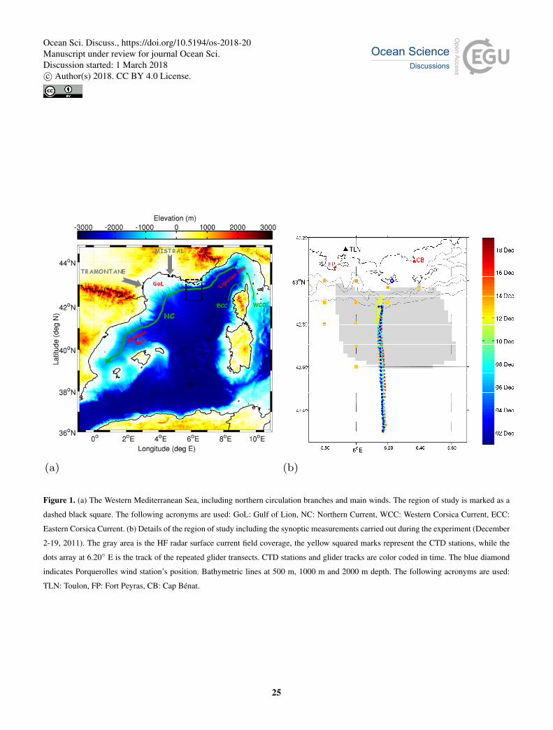
(a) (b)
Figure 1. (a) The Western Mediterranean Sea, including northern circulation branches and main winds. The region of study is marked as a
dashed black square. The following acronyms are used: GoL: Gulf of Lion, NC: Northern Current, WCC: Western Corsica Current, ECC:
Eastern Corsica Current. (b) Details of the region of study including the synoptic measurements carried out during the experiment (December
2-19, 2011). The gray area is the HF radar surface current field coverage, the yellow squared marks represent the CTD stations, while the
dots array at 6.20◦ E is the track of the repeated glider transects. CTD stations and glider tracks are color coded in time. The blue diamond
indicates Porquerolles wind station’s position. Bathymetric lines at 500 m, 1000 m and 2000 m depth. The following acronyms are used:
TLN: Toulon, FP: Fort Peyras, CB: Cap Bénat.
25
Ocean Sci. Discuss., https://doi.org/10.5194/os-2018-20Manuscript under review for journal Ocean Sci.Discussion started: 1 March 2018c© Author(s) 2018. CC BY 4.0 License.

02 03 04 05 06 07 08 09 10 11 12 13 14 15 16 17 18 190
4
8
12
16
20
empt
y pa
nel
02 03 04 05 06 07 08 09 10 11 12 13 14 15 16 17 18 19
Observations time line
December 2011
02 03 04 05 06 07 08 09 10 11 12 13 14 15 16 17 18 19
(a)
02 03 04 05 06 07 08 09 10 11 12 13 14 15 16 17 18 190
4
8
12
16
20Winds over HFR field
spee
d (m
/s)
E1 E2 E3
02 03 04 05 06 07 08 09 10 11 12 13 14 15 16 17 18 19E
N
W
S
E
dire
ctio
n (b
low
ing
from
)
December 2011
Porquerolles station
ALADIN model
(b)
Figure 2. (a) The multi-platform observations time line: the black dashed lines indicate the selected wind events (compare with panel below),
the gray area indicates the radar dataset availability, the red areas indicate the glider transects, and the green dashed lines indicate the period in
which the glider transects fall inside the HFR coverage. (b) Wind time series from Porquerolles wind station (blue line) and from ALADIN
model (black line) are compared in terms of speed (middle panel) and direction (bottom panel). The limits of the selected wind events
(speed>10ms−1, gray line in the middle panel) are indicated with red dashed lines and named E1, E2, and E3.
26
Ocean Sci. Discuss., https://doi.org/10.5194/os-2018-20Manuscript under review for journal Ocean Sci.Discussion started: 1 March 2018c© Author(s) 2018. CC BY 4.0 License.
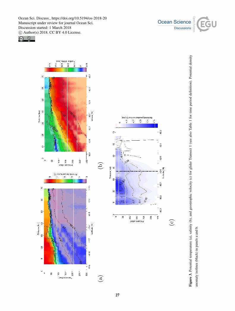
(a)
(b)
(c)
Figu
re3.
Pote
ntia
ltem
pera
ture
(a),
salin
ity(b
),an
dge
ostr
ophi
cve
loci
ty(c
)fo
rgl
ider
Tran
sect
1(s
eeal
soTa
ble
1fo
rtim
epe
riod
defin
ition
).Po
tent
iald
ensi
ty
anom
aly
isol
ines
(bla
ck)i
npa
nels
aan
db.
27
Ocean Sci. Discuss., https://doi.org/10.5194/os-2018-20Manuscript under review for journal Ocean Sci.Discussion started: 1 March 2018c© Author(s) 2018. CC BY 4.0 License.

(a)
(b)
(c)
5.8
0
6o E
6.2
0 6
.40
6.6
0 4
2.50
42.
60
42.
70
42.
80
42.
90
43o N
0.
5 m
/s
10 m
/s (
win
d)
Ave
rage
cur
rent
s an
d w
ind
(07−
08−
Dec
−20
11)
(d)
Figu
re4.
Pote
ntia
ltem
pera
ture
(a),
salin
ity(b
),an
dge
ostr
ophi
cve
loci
ty(c
)fo
rgl
ider
Tran
sect
3(s
eeal
soTa
ble
1fo
rtim
epe
riod
defin
ition
).Po
tent
iald
ensi
ty
anom
aly
isol
ines
(bla
ck)
inpa
nels
aan
db.
The
blac
kda
shed
line
(pan
elc)
repr
esen
tsth
eso
uthe
rnbo
unda
ryof
the
HF
rada
rfie
ld.I
npa
nel(
d),b
lack
arro
ws
are
the
surf
ace
curr
ents
from
HFR
aver
aged
duri
ngth
epe
riod
inw
hich
the
glid
ertr
anse
ct(g
reen
dash
edlin
e)fa
llsin
side
the
HFR
cove
rage
(and
cons
ider
ing
only
grid
poin
tsw
ithat
leas
t80%
avai
labl
eda
taov
erth
etim
epe
riod
).T
hebl
uear
row
repr
esen
tthe
win
dfr
omPo
rque
rolle
sst
atio
nav
erag
edov
erth
esa
me
peri
odco
nsid
ered
fort
heH
FRav
erag
e.
28
Ocean Sci. Discuss., https://doi.org/10.5194/os-2018-20Manuscript under review for journal Ocean Sci.Discussion started: 1 March 2018c© Author(s) 2018. CC BY 4.0 License.
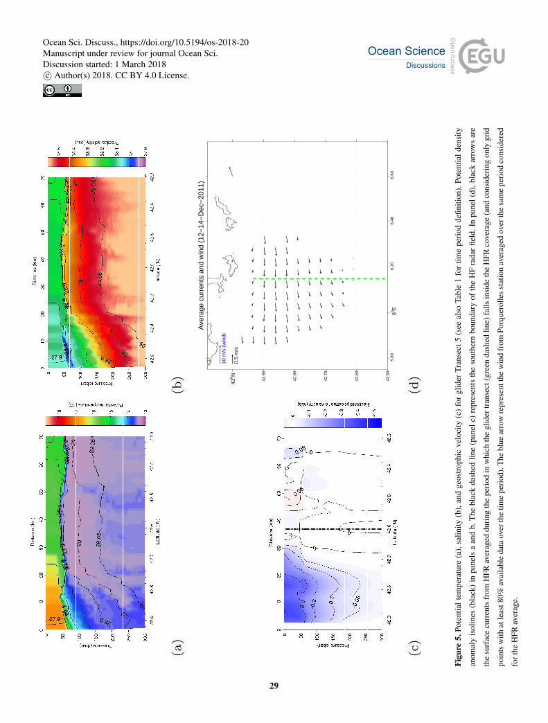
(a)
(b)
(c)
5.8
0
6o E
6.2
0 6
.40
6.6
0 4
2.50
42.
60
42.
70
42.
80
42.
90
43o N
0.
5 m
/s
10 m
/s (
win
d)
Ave
rage
cur
rent
s an
d w
ind
(12−
14−
Dec
−20
11)
(d)
Figu
re5.
Pote
ntia
ltem
pera
ture
(a),
salin
ity(b
),an
dge
ostr
ophi
cve
loci
ty(c
)fo
rgl
ider
Tran
sect
5(s
eeal
soTa
ble
1fo
rtim
epe
riod
defin
ition
).Po
tent
iald
ensi
ty
anom
aly
isol
ines
(bla
ck)
inpa
nels
aan
db.
The
blac
kda
shed
line
(pan
elc)
repr
esen
tsth
eso
uthe
rnbo
unda
ryof
the
HF
rada
rfie
ld.I
npa
nel(
d),b
lack
arro
ws
are
the
surf
ace
curr
ents
from
HFR
aver
aged
duri
ngth
epe
riod
inw
hich
the
glid
ertr
anse
ct(g
reen
dash
edlin
e)fa
llsin
side
the
HFR
cove
rage
(and
cons
ider
ing
only
grid
poin
tsw
ithat
leas
t80%
avai
labl
eda
taov
erth
etim
epe
riod
).T
hebl
uear
row
repr
esen
tthe
win
dfr
omPo
rque
rolle
sst
atio
nav
erag
edov
erth
esa
me
peri
odco
nsid
ered
fort
heH
FRav
erag
e.
29
Ocean Sci. Discuss., https://doi.org/10.5194/os-2018-20Manuscript under review for journal Ocean Sci.Discussion started: 1 March 2018c© Author(s) 2018. CC BY 4.0 License.
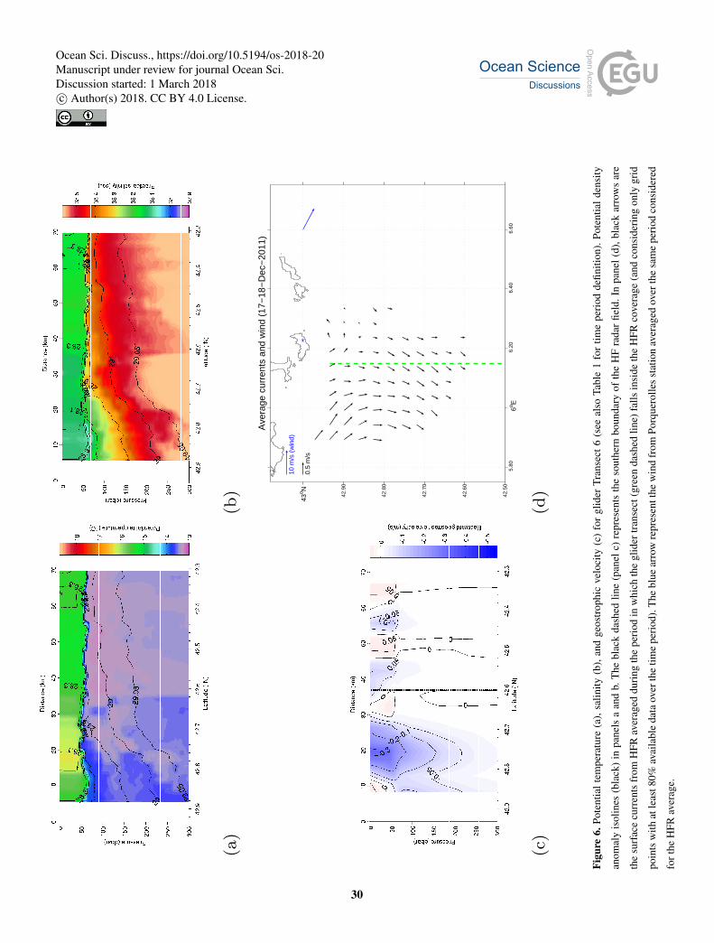
(a)
(b)
(c)
5.8
0
6o E
6.2
0 6
.40
6.6
0 4
2.50
42.
60
42.
70
42.
80
42.
90
43o N
0.
5 m
/s
10 m
/s (
win
d)
Ave
rage
cur
rent
s an
d w
ind
(17−
18−
Dec
−20
11)
(d)
Figu
re6.
Pote
ntia
ltem
pera
ture
(a),
salin
ity(b
),an
dge
ostr
ophi
cve
loci
ty(c
)fo
rgl
ider
Tran
sect
6(s
eeal
soTa
ble
1fo
rtim
epe
riod
defin
ition
).Po
tent
iald
ensi
ty
anom
aly
isol
ines
(bla
ck)
inpa
nels
aan
db.
The
blac
kda
shed
line
(pan
elc)
repr
esen
tsth
eso
uthe
rnbo
unda
ryof
the
HF
rada
rfie
ld.I
npa
nel(
d),b
lack
arro
ws
are
the
surf
ace
curr
ents
from
HFR
aver
aged
duri
ngth
epe
riod
inw
hich
the
glid
ertr
anse
ct(g
reen
dash
edlin
e)fa
llsin
side
the
HFR
cove
rage
(and
cons
ider
ing
only
grid
poin
tsw
ithat
leas
t80%
avai
labl
eda
taov
erth
etim
epe
riod
).T
hebl
uear
row
repr
esen
tthe
win
dfr
omPo
rque
rolle
sst
atio
nav
erag
edov
erth
esa
me
peri
odco
nsid
ered
fort
heH
FRav
erag
e.
30
Ocean Sci. Discuss., https://doi.org/10.5194/os-2018-20Manuscript under review for journal Ocean Sci.Discussion started: 1 March 2018c© Author(s) 2018. CC BY 4.0 License.

0 10 20 30 40 50 60 700
20
40
60
80
100
120
140
160
Pre
ssur
e (d
bar)
Distance (km)
42.9 42.8 42.7 42.6 42.5 42.4 42.3
0
20
40
60
80
100
120
140
160
Pre
ssur
e (d
bar)
Latitude (°N)42.9 42.8 42.7 42.6 42.5 42.4 42.3
0
20
40
60
80
100
120
140
160
Pre
ssur
e (d
bar)
Latitude (°N)42.9 42.8 42.7 42.6 42.5 42.4 42.3
0
20
40
60
80
100
120
140
160
Pre
ssur
e (d
bar)
Latitude (°N)42.9 42.8 42.7 42.6 42.5 42.4 42.3
0
20
40
60
80
100
120
140
160
Pre
ssur
e (d
bar)
Latitude (°N)42.9 42.8 42.7 42.6 42.5 42.4 42.3
0
20
40
60
80
100
120
140
160
Pre
ssur
e (d
bar)
Latitude (°N)Latitude (°N)42.9 42.8 42.7 42.6 42.5 42.4 42.3
0
20
40
60
80
100
120
140
160
Transect 1
Transect 2
Transect 3
Transect 4
Transect 5
Transect 6
Figure 7. Potential density anomaly σ(z)=28.7 kg/m3 isopycnal evolution color coded for each glider transect.
31
Ocean Sci. Discuss., https://doi.org/10.5194/os-2018-20Manuscript under review for journal Ocean Sci.Discussion started: 1 March 2018c© Author(s) 2018. CC BY 4.0 License.

Figure 8. Cross-shore NC transport computed from glider relative geostrophic velocity profiles (reference pressure at 500 mbar) for each
glider transect.
32
Ocean Sci. Discuss., https://doi.org/10.5194/os-2018-20Manuscript under review for journal Ocean Sci.Discussion started: 1 March 2018c© Author(s) 2018. CC BY 4.0 License.

42.642.6542.742.7542.842.8542.9−0.5
−0.4
−0.3
−0.2
−0.1
0
0.1
0.2
0.3
0.4
0.5
Latitude (° N)
velo
city
(m
/s)
Surface velocity components, Transect 2
u geo glideru HFRv HFR
(a)
42.642.6542.742.7542.842.8542.9−0.5
−0.4
−0.3
−0.2
−0.1
0
0.1
0.2
0.3
0.4
0.5
Latitude (° N)
velo
city
(m
/s)
Surface velocity components, Transect 3
u geo glideru HFRv HFR
(b)
42.642.6542.742.7542.842.8542.9−0.5
−0.4
−0.3
−0.2
−0.1
0
0.1
0.2
0.3
0.4
0.5
Latitude (° N)
velo
city
(m
/s)
Surface velocity components, Transect 4
u geo glideru HFRv HFR
(c)
42.642.6542.742.7542.842.8542.9−0.5
−0.4
−0.3
−0.2
−0.1
0
0.1
0.2
0.3
0.4
0.5
Latitude (° N)
velo
city
(m
/s)
Surface velocity components, Transect 5
u geo glideru HFRv HFR
(d)
42.642.6542.742.7542.842.8542.9−0.5
−0.4
−0.3
−0.2
−0.1
0
0.1
0.2
0.3
0.4
0.5
Latitude (° N)
velo
city
(m
/s)
Surface velocity components, Transect 6
u geo glideru HFRv HFR
(e)
Figure 9. Comparison of uS (solid black line) and vS (dashed black line) components of total surface currents from HFR and uSg (green
line) geostrophic component from glider transects. Positive u (v) currents are eastward (northward), and the gray line indicates null velocities.
Panels (a) to (e) represent measurements during Transects 2 to 6.
33
Ocean Sci. Discuss., https://doi.org/10.5194/os-2018-20Manuscript under review for journal Ocean Sci.Discussion started: 1 March 2018c© Author(s) 2018. CC BY 4.0 License.
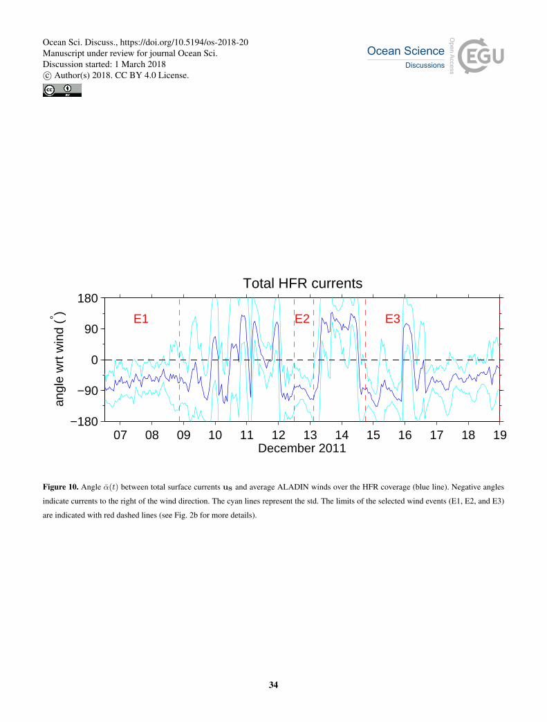
07 08 09 10 11 12 13 14 15 16 17 18 19−180
−90
0
90
180
E1 E2 E3
Total HFR currents
angl
e w
rt w
ind
(° )
December 2011
07 08 09 10 11 12 13 14 15 16 17 18 19−180
−90
0
90
180
empt
y pa
nel
Figure 10. Angle α(t) between total surface currents uS and average ALADIN winds over the HFR coverage (blue line). Negative angles
indicate currents to the right of the wind direction. The cyan lines represent the std. The limits of the selected wind events (E1, E2, and E3)
are indicated with red dashed lines (see Fig. 2b for more details).
34
Ocean Sci. Discuss., https://doi.org/10.5194/os-2018-20Manuscript under review for journal Ocean Sci.Discussion started: 1 March 2018c© Author(s) 2018. CC BY 4.0 License.

5.80 6oE 6.20 6.40 6.60 42.50
42.60
42.70
42.80
42.90
43oN 0.5 m/s
Reference geostrophic currents (12−Dec−2011 00−06 h)
(a)
5.80 6oE 6.20 6.40 6.60 42.50
42.60
42.70
42.80
42.90
43oN
0.5 m/s
HFR field (12−Dec−2011 14:00:00)
(b)
5.80 6oE 6.20 6.40 6.60 42.50
42.60
42.70
42.80
42.90
43oN 5 m/s
Model wind field (12−Dec−2011 14:00:00)
(c)
Wind and ageostrophic currents (12−Dec−2011 14:00:00)
5.80 6oE 6.20 6.40 6.60 42.50
42.60
42.70
42.80
42.90
43oN
0.5 m/s
angl
e be
twee
n w
ind
and
ageo
stro
phic
cur
rent
(° )
−150
−100
−50
0
50
100
150
(d)
Figure 11. Example maps of: (a) 6h time-averaged geostrophic flow uSg derived from HFR, (b) instaneous HFR surface currents uS, (c)
ALADIN wind field, and (d) ageostrophic surface currents uSaW superimposed on the color coded map quantifying the angle α between the
ageostrophic component and ALADIN wind. Negative values means current to the right of the wind.
35
Ocean Sci. Discuss., https://doi.org/10.5194/os-2018-20Manuscript under review for journal Ocean Sci.Discussion started: 1 March 2018c© Author(s) 2018. CC BY 4.0 License.
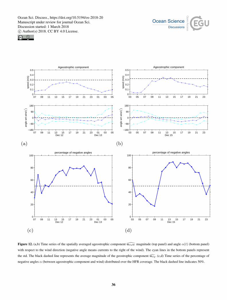
07 09 11 13 15 17 19 21 23 01 03 050
0.1
0.2
0.3
0.4
0.5Ageostrophic component
spee
d (m
/s)
07 09 11 13 15 17 19 21 23 01 03 05−180
−90
0
90
180
angl
e w
rt w
ind
(° )
Dec 12 Dec 13
(a)
03 05 07 09 11 13 15 17 19 21 230
0.1
0.2
0.3
0.4
0.5Ageostrophic component
spee
d (m
/s)
03 05 07 09 11 13 15 17 19 21 23−180
−90
0
90
180
angl
e w
rt w
ind
(° )
Dec 15
(b)
07 09 11 13 15 17 19 21 23 01 03 050
20
40
60
80
100percentage of negative angles
Dec 12 Dec 13
(c)
03 05 07 09 11 13 15 17 19 21 230
20
40
60
80
100percentage of negative angles
Dec 15
(d)
Figure 12. (a,b) Time series of the spatially averaged ageostrophic component uSaW magnitude (top panel) and angle α(t) (bottom panel)
with respect to the wind direction (negative angle means currents to the right of the wind). The cyan lines in the bottom panels represent
the std. The black dashed line represents the average magnitude of the geostrophic component uSg . (c,d) Time series of the percentage of
negative angles α (between ageostrophic component and wind) distributed over the HFR coverage. The black dashed line indicates 50%.
36
Ocean Sci. Discuss., https://doi.org/10.5194/os-2018-20Manuscript under review for journal Ocean Sci.Discussion started: 1 March 2018c© Author(s) 2018. CC BY 4.0 License.
Recommended