Embed Size (px)
Citation preview

ENSO-Like and ENSO-Induced Tropical Pacific Decadal Variability in CGCMs
JUNG CHOI AND SOON-IL AN
Department of Atmospheric Sciences, Yonsei University, Seoul, South Korea
SANG-WOOK YEH
Department of Environmental Marine Science, Hanyang University, Ansan, South Korea
JIN-YI YU
Department of Earth System Science, University of California, Irvine, Irvine, California
(Manuscript received 19 February 2012, in final form 26 July 2012)
ABSTRACT
Outputs from coupled general circulation models (CGCMs) are used in examining tropical Pacific
decadal variability (TPDV) and their relationships with El Nino–Southern Oscillation (ENSO). Herein
TPDV is classified as either ENSO-induced TPDV (EIT) or ENSO-like TPDV (ELT), based on their
correlations with a decadal modulation index of ENSO amplitude and spatial pattern. EIT is identified
by the leading EOF mode of the low-pass filtered equatorial subsurface temperature anomalies and is
highly correlated with the decadal ENSO modulation index. This mode is characterized by an east–west
dipole structure along the equator. ELT is usually defined by the first EOF mode of subsurface tem-
perature, of which the spatial structure is similar to ENSO. Generally, this mode is insignificantly
correlated with the decadal modulation of ENSO. EIT closely interacts with the residuals induced by
ENSO asymmetries, both of which show similar spatial structures. On the other hand, ELT is controlled
by slowly varying ocean adjustments analogous to a recharge oscillator of ENSO. Both types of TPDV
have similar spectral peaks on a decadal-to-interdecadal time scale. Interestingly, the variances of both
types of TPDV depend on the strength of connection between El Nino–La Nina residuals and EIT, such
that the strong two-way feedback between them enhances EIT and reduces ELT. The strength of the
two-way feedback is also related to ENSO variability. The flavors of El Nino–La Nina with respect to
changes in the tropical Pacific mean state tend to be well simulated when ENSO variability is larger in
CGCMs. As a result, stronger ENSO variability leads to intensified interactive feedback between
ENSO residuals and enhanced EIT in CGCMs.
1. Introduction
Tropical Pacific decadal variability (TPDV) is an im-
portant component of global-scale climate variability
(Mantua et al. 1997; Zhang et al. 1997), which is known to
be related to the Pacific–NorthAmerica pattern (Wallace
and Gutzler 1981) in the Northern Hemisphere as well
as the atmospheric circulation near the Southern
Ocean and Antarctica (Garreaud and Battisti 1999).
The dominant mode of TPDV is characterized by broad
triangular-shaped sea surface temperature (SST) varia-
tions exhibiting a warmer than normal tropical central-
to-eastern Pacific and a colder than normal extratropical
central North Pacific or vice versa (Latif et al. 1997). The
SST variations associated with TPDV have been de-
tected in observations (Evans et al. 2002). In the mid-
1970s, a distinctive triangular-shaped SST warming
anomaly pattern existed in the tropical eastern Pacific
(Zhang et al. 1997; Luo and Yamagata 2001; Ashok et al.
2007). This decadal variability shows a structure largely
similar to El Nino–Southern Oscillation (ENSO) in the
tropical Pacific, yet this type of structure is typically more
prominent over the extratropical North Pacific (Zhang
et al. 1997). Many previous studies (Knutson andManabe
1998; Luo et al. 2003; Wang et al. 2003) have documented
Corresponding author address: Prof. Soon-Il An, Department of
Atmospheric Sciences, Yonsei University, Seoul 120-749, South
Korea.
E-mail: [email protected]
1 MARCH 2013 CHO I ET AL . 1485
DOI: 10.1175/JCLI-D-12-00118.1
� 2013 American Meteorological Society
that a slow ocean adjustment process on a decadal-to-
interdecadal time scale accounts for phase transition
analogous to the recharge/discharge oscillator of ENSO
(Jin 1997a,b). Therefore, this TPDV is usually known as
‘‘ENSO-like tropical Pacific decadal variability.’’ This is
the most dominant mode of equatorial Pacific temper-
ature variation on a decadal-to-interdecadal time scale.
Meanwhile, ENSO properties, including amplitude,
frequency, and spatial distribution, vary on a decadal-to-
interdecadal time scale (An 2004, 2009; Sun and Yu
2009; Choi et al. 2011). This decadal modulation of
ENSO properties has been explained by several differ-
ent theories. On the one hand, some studies (Zebiak
1989; Jin et al. 1994; Timmermann 2003) have empha-
sized the nonlinear internal dynamics of the coupled
tropical system as the basis for the modulation, and
others (Kirtman and Schopf 1998; Flugel and Chang
1999; Burgman et al. 2008) have proposed the impor-
tance of stochastic forcing generated by the atmospheric
noise. On the other hand, other studies have pointed out
that changes in the tropical Pacific mean state could lead
to changes in ENSO properties (An and Wang 2000;
Fedorov and Philander 2000; An et al. 2006; Dewitte
et al. 2007; Bejarano and Jin 2008). In other words, the
change in mean state associated with TPDV appears to
be a plausible reason for decadal ENSO modulation
(Choi et al. 2009; Li et al. 2011; Yu and Kim 2011).
However, another study demonstrated that there is little
or no relationship between the ENSO-like TPDV and
decadal modulation of ENSO in CGCM (Yeh and
Kirtman 2004). Instead, the second mode of TPDV is
more closely related to decadal ENSO modulation. The
spatial pattern of the second empirical orthogonal
function (EOF) mode is quite different from the ENSO-
like TPDV pattern. Timmermann (2003) has also
pointed out that the second EOF mode, which reflects
subsurface temperature anomalies in the equatorial
Pacific that exhibit an east–west dipole-like structure,
are strongly related to decadal ENSO modulation.
Furthermore, Sun and Yu (2009) demonstrated that
observed TPDV with a notable east–west dipole-like
spatial structure could be induced by the rectification
effect of ENSO. Also, Dewitte et al. (2009) studied the
relationship between the first two EOF modes of low-
frequency subsurface temperature and the ENSO mod-
ulation from the SODA reanalysis data. In this regard,
the decadal modulation of ENSO does not appear to be
related to the ENSO-like mode but rather the dipole-like
mode of TPDV.
The origin of the dipole-like mode of TPDV is sug-
gested to be the statistical residual for asymmetric
anomaly patterns associated with El Nino and La Nina
events (Rodgers et al. 2004; Cibot et al. 2005; Schopf
and Burgman 2006; Sun and Yu 2009). Those studies
demonstrated that the residuals, owing to asymmetries
between El Nino and La Nina in their spatial patterns
and amplitudes, could rectify into a background condi-
tion and lead a slowly varying variability. Using high-
quality and in situ ocean datasets, McPhaden et al.
(2011) recently argued that decadal change in the trop-
ical Pacific SST during the 2000s, resembling a dipole-
like structure, is due to a greater occurrence of central
Pacific warming events—for example, central Pacific El
Nino (Yu and Kao 2007; Kao and Yu 2009; Yeh et al.
2009), warm pool El Nino (Kug et al. 2009), and El Nino
Modoki (Ashok et al. 2007)—but not the other way
around. Likewise, Choi et al. (2012) argued that the
statistical residuals as a result of El Nino–La Nina
asymmetry representing an east–west dipole structure
could feed into the tropical Pacific mean state. In-
terestingly, both the residual pattern due to ENSO
asymmetry and the mean state pattern correlated to
the decadal modulation of ENSO show similar east–
west dipole-like structures, suggesting a strong dynamic
relationship between them that is worthy of further
investigation.
According to these previous studies, at least two types
of TPDVs exist. One is ENSO-like TPDV, which has
a spatial structure resembling ENSO (i.e., triangular
structure in SST anomaly; referred to as ENSO-like
TPDV). The other type is related to decadal ENSO
modulation, which has an east–west dipole structure in
the tropical Pacific (referred to as ENSO-induced
TPDV). Several studies demonstrating the relationship
between these two types of TPDVs have been con-
ducted. Yeh and Kirtman (2004) demonstrated that
ENSO-like TPDV accounts for a larger percentage
variance of decadal SST variability than does ENSO-
induced TPDV in a coupled general circulation model
(CGCM). They also showed that the variance of ENSO-
like TPDV grew larger as the amplitude of atmospheric
noise increased. Choi et al. (2012) demonstrated that
ENSO-induced TPDV somehow experienced a phase
transition of ENSO-like TPDV. That study’s results
imply that these two types of TPDVs are linearly in-
dependent but related. Nevertheless, their relationship
is not yet fully understood. Furthermore, it is unclear
why different CGCMs produce different relative
strengths of these two TPDV types (e.g., Yu and Kim
2011).
Overall, the primary interest of this study is to ex-
amine the relationship between ENSO-like and ENSO-
inducedTPDVs inCGCMs. Furthermore, the associations
between both TPDV modes and the simulated ENSO
will be investigated. Section 2 describes the datasets and
CGCMs used in this study. Section 3 describes the
1486 JOURNAL OF CL IMATE VOLUME 26
classification of the two TPDVs in the CGCMs and
their spatial characteristics. Section 4 shares details on
the relationship between the two TPDVs and ENSO,
and section 5 provides a summary and discussion of the
study.
2. Data
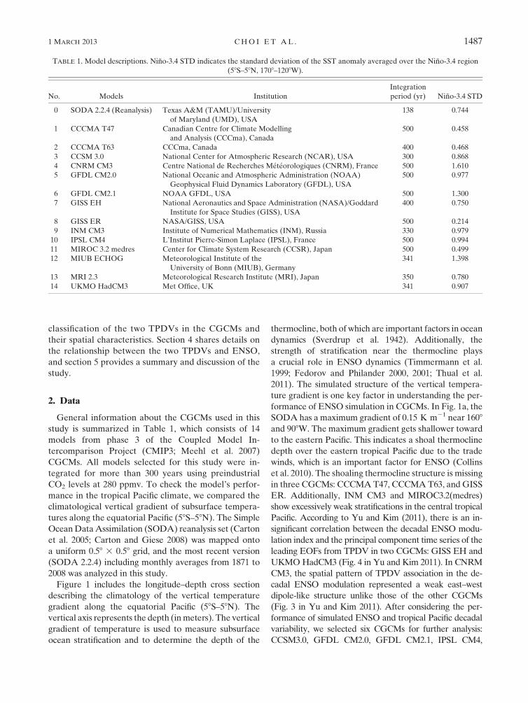
General information about the CGCMs used in this
study is summarized in Table 1, which consists of 14
models from phase 3 of the Coupled Model In-
tercomparison Project (CMIP3; Meehl et al. 2007)
CGCMs. All models selected for this study were in-
tegrated for more than 300 years using preindustrial
CO2 levels at 280 ppmv. To check the model’s perfor-
mance in the tropical Pacific climate, we compared the
climatological vertical gradient of subsurface tempera-
tures along the equatorial Pacific (58S–58N). The Simple
OceanDataAssimilation (SODA) reanalysis set (Carton
et al. 2005; Carton and Giese 2008) was mapped onto
a uniform 0.58 3 0.58 grid, and the most recent version
(SODA 2.2.4) including monthly averages from 1871 to
2008 was analyzed in this study.
Figure 1 includes the longitude–depth cross section
describing the climatology of the vertical temperature
gradient along the equatorial Pacific (58S–58N). The
vertical axis represents the depth (inmeters). The vertical
gradient of temperature is used to measure subsurface
ocean stratification and to determine the depth of the
thermocline, both of which are important factors in ocean
dynamics (Sverdrup et al. 1942). Additionally, the
strength of stratification near the thermocline plays
a crucial role in ENSO dynamics (Timmermann et al.
1999; Fedorov and Philander 2000, 2001; Thual et al.
2011). The simulated structure of the vertical tempera-
ture gradient is one key factor in understanding the per-
formance of ENSO simulation in CGCMs. In Fig. 1a, the
SODA has a maximum gradient of 0.15 K m21 near 1608and 908W. The maximum gradient gets shallower toward
to the eastern Pacific. This indicates a shoal thermocline
depth over the eastern tropical Pacific due to the trade
winds, which is an important factor for ENSO (Collins
et al. 2010). The shoaling thermocline structure is missing
in three CGCMs: CCCMAT47, CCCMAT63, and GISS
ER. Additionally, INM CM3 and MIROC3.2(medres)
show excessively weak stratifications in the central tropical
Pacific. According to Yu and Kim (2011), there is an in-
significant correlation between the decadal ENSO modu-
lation index and the principal component time series of the
leading EOFs from TPDV in two CGCMs: GISS EH and
UKMOHadCM3 (Fig. 4 in Yu and Kim 2011). In CNRM
CM3, the spatial pattern of TPDV association in the de-
cadal ENSO modulation represented a weak east–west
dipole-like structure unlike those of the other CGCMs
(Fig. 3 in Yu and Kim 2011). After considering the per-
formance of simulated ENSO and tropical Pacific decadal
variability, we selected six CGCMs for further analysis:
CCSM3.0, GFDL CM2.0, GFDL CM2.1, IPSL CM4,
TABLE 1. Model descriptions. Nino-3.4 STD indicates the standard deviation of the SST anomaly averaged over the Nino-3.4 region
(58S–58N, 1708–1208W).
No. Models Institution
Integration
period (yr) Nino-3.4 STD
0 SODA 2.2.4 (Reanalysis) Texas A&M (TAMU)/University
of Maryland (UMD), USA
138 0.744
1 CCCMA T47 Canadian Centre for Climate Modelling
and Analysis (CCCma), Canada
500 0.458
2 CCCMA T63 CCCma, Canada 400 0.468
3 CCSM 3.0 National Center for Atmospheric Research (NCAR), USA 300 0.868
4 CNRM CM3 Centre National de Recherches Meteorologiques (CNRM), France 500 1.610
5 GFDL CM2.0 National Oceanic and Atmospheric Administration (NOAA)
Geophysical Fluid Dynamics Laboratory (GFDL), USA
500 0.977
6 GFDL CM2.1 NOAA GFDL, USA 500 1.300
7 GISS EH National Aeronautics and Space Administration (NASA)/Goddard
Institute for Space Studies (GISS), USA
400 0.750
8 GISS ER NASA/GISS, USA 500 0.214
9 INM CM3 Institute of Numerical Mathematics (INM), Russia 330 0.979
10 IPSL CM4 L’Institut Pierre-Simon Laplace (IPSL), France 500 0.994
11 MIROC 3.2 medres Center for Climate System Research (CCSR), Japan 500 0.499
12 MIUB ECHOG Meteorological Institute of the
University of Bonn (MIUB), Germany
341 1.398
13 MRI 2.3 Meteorological Research Institute (MRI), Japan 350 0.780
14 UKMO HadCM3 Met Office, UK 341 0.907
1 MARCH 2013 CHO I ET AL . 1487

MIUB ECHOG, and MRI 2.3. The selected CGCMs will
be analyzed in the next several sections based on the re-
lationship between ENSO and tropical Pacific decadal
variability and the possible mechanisms.
3. Two modes of TPDVs in CGCMs
To identify TPDVs in the CGCMs, we performed an
empirical orthogonal function analysis (also known as
principal component analysis) of equatorial (58S–58N)
subsurface temperature anomalies from the surface to
a 250-m depth. Previous studies used SST anomalies to
identify ENSO or TPDV (Yu and Boer 2004; Imada and
Kimoto 2009; Yu and Kim 2011). In this study, we used
averaged subsurface temperature anomalies of the
equator, as suggested in Choi et al. (2011, 2012), to
identify subsurface ocean structures that store long-term
memory for climate variability. The anomalies were
FIG. 1. Longitude–depth cross section of the climatology of the vertical temperature gradient (58S–58N).
1488 JOURNAL OF CL IMATE VOLUME 26
detected by removing seasonal climatology. The first
columns in Fig. 2 show the spatial patterns of the first
leading EOF modes from the six selected CGCMs.
These leading modes have a spectral peak near the in-
terannual band (not shown), which is related to the
ENSO time scale. In the first columns of Fig. 3, re-
gressions of tropical Pacific SST anomalies associated
with the principal components of these leading EOF
modes further confirm that the leading modes of Fig. 2
are the simulated ENSO in the CGCMs. Figure 3
demonstrates that the SST anomaly center of the sim-
ulated ENSO tends to be located more westward com-
pared to the observations, which is a model deficiency
common to many CGCMs due to a strong simulated
cold tongue (Latif et al. 2001; AchutaRao and Sperber
2002; Hannachi et al. 2003). Nevertheless, the general
features of the simulated ENSO are reasonably realistic
compared with observations that indicate a large posi-
tive anomaly over the equatorial region and a weak
negative anomaly over the western off-equatorial re-
gion. The ENSO simulated in GFDL CM2.1 and MIUB
ECHOG is stronger than that of other models. The
structures shown in the first columns of Fig. 2 represent
the subsurface ocean structure during the peak phase of
El Nino events. There is basin-scale warming at the
surface and a dipole structure along the thermocline
depth. These features are consistent with the conven-
tional characteristics of El Nino, including a deeper
mean thermocline depth and accumulated heat content
over the eastern tropical Pacific (Jin 1997a,b).
A 10-yr sliding average was applied to the ocean
temperature anomalies to obtain decadal variability. An
EOF analysis was then applied to the decadal anomalies
to obtain leading modes of TPDV. To identify the
ENSO-induced mode of TPDV, we defined a decadal
modulation index of ENSO amplitude, which is calcu-
lated as the 10-yr sliding standard deviation for the
Nino-3.4 (averaged over 58S–58N, 1708–1208W) SST
anomalies. We then calculated the temporal correlation
between the decadal modulation index of ENSO and the
principal component (PC) time series of the leading
decadal modes of TPDV. The EOF mode with the
highest temporal correlation was classified as the
ENSO-induced TPDV. The second column in Fig. 2
displays the ENSO-induced TPDV from the six selected
CGCMs. As demonstrated in the figures, the longitude–
depth structure of ENSO-induced TPDV is character-
ized by an east–west dipole structure. This feature is
generally simulated by the six CGCMs, with the ex-
ception of CCSM3.0, which has a weak warming on the
eastern side. The percentage of variance (%) explained
by these modes and their temporal correlations with the
decadal ENSO modulation index are listed in Table 2.
The temporal correlations are statistically significant at
99% in all six CGCMs. The GFDL CM2.1 and MIUB
ECHOG simulated the ENSO-induced TPDV as the
first leading mode of TPDV, with more than 50% of the
variance explained by this mode. In the other models
(CCSM3.0, GFDL CM2.0, IPSL CM4, and MRI2.3),
ENSO-induced TPDV is either the second or third
mode of TPDV, explaining less than 30% of the decadal
variance. When we consider another index for ENSO
amplitude modulation such as N3Var index (Cibot et al.
2005), the temporal correlations are not significantly
changed.
The third column of Fig. 2 demonstrates that the first
mode in the decadal EOF analysis is not an ENSO-
induced mode. In the cases of GFDL CM2.1 and MIUB
ECHOG, this mode is the second leading mode of the
EOF analysis, and the first EOF mode is the ENSO-
induced TPDV. In the cases of CCSM3.0, GFDLCM2.0,
IPSL CM4, and MRI2.3, this mode is the first leading
mode from the EOF analysis. It should be noted that, in
the GFDL CM2.0, the first and second modes described
the same decadal variability because the second EOF
mode represented the transition phase of the first EOF
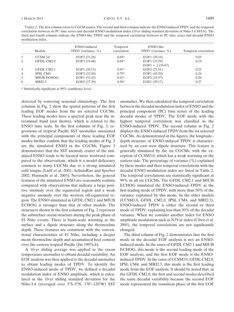
TABLE 2. The first column refers to CGCM names. The second and third columns indicate the ENSO-induced TPDV and the temporal
correlation between its PC time series and decadal ENSO modulation index (10-yr sliding standard deviation of Nino-3.4 SSTA). The
third and fourth columns indicate the ENSO-like TPDV and the temporal correlation between its PC time series and decadal ENSO
modulation index.
Models
ENSO-induced
TPDV (variance, %)
Temporal
correlation
ENSO-like
TPDV (variance, %) Temporal correlation
1 CCSM 3.0 EOF2 (23.28) 0.69* EOF1 (39.19) 0.03
2 GFDL CM2.0 EOF3 (19.48) 0.84* EOF1 (33.59) 0.19
EOF1 1 2 (59.67)
3 GFDL CM2.1 EOF1 (59.13) 0.91* EOF2 (21.51) 0.23
4 IPSL CM4 EOF2 (23.50) 0.79* EOF1 (43.20) 0.24
5 MIUB ECHOG EOF1 (53.43) 0.91* EOF2 (19.57) 0.20
6 MRI2.3 EOF2 (27.39) 0.56* EOF1 (39.17) 0.27
* Statistically significant at 99% confidence level.
1 MARCH 2013 CHO I ET AL . 1489
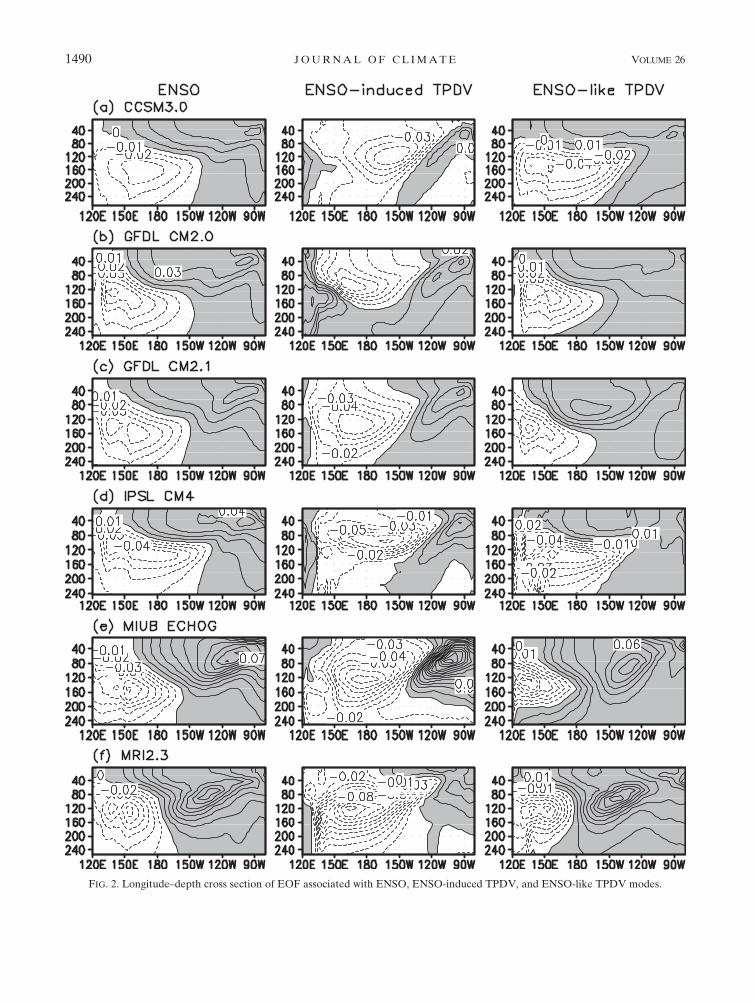
FIG. 2. Longitude–depth cross section of EOF associated with ENSO, ENSO-induced TPDV, and ENSO-like TPDV modes.
1490 JOURNAL OF CL IMATE VOLUME 26

mode. All of the modes shown in the third column of
Fig. 2 have a vertical structure similar to that shown for
the ENSO (i.e., the first column of Fig. 2). The pattern
correlations between these two columns of Fig. 2 are
0.90 for CCSM3.0, 0.97 for GFDL CM2.0, 0.73 for
GFDL CM2.1, 0.92 for IPSL CM4, 0.80 for MIUB
ECHOG, and 0.92 for MRI2.3. Therefore, we identified
this mode to be the ENSO-like TPDV. This mode has
a structure similar to ENSO, but the centers of warm
anomalies move to the west compared to those of
ENSO. The center of the subsurface temperature
anomalies of ENSO-like TPDV is located farther west
than in the ENSO mode. The ENSO-like TPDV plays
an important role in the stratification of the central Pa-
cific, as exhibited by opposite anomalies between the
surface and subsurface. The temporal correlations
FIG. 3. Regressed map of SST associated with the EOF PC time series of ENSO, ENSO-induced TPDV, and ENSO-like
TPDV modes (K).
1 MARCH 2013 CHO I ET AL . 1491
between the PCs of these modes and the decadal ENSO
modulation index are listed in Table 2. The ENSO-like
TPDV has a weak or no relationship with the decadal
modulation of ENSO amplitude, despite their similar
spatial structures. This result is consistent with the result
of Yeh and Kirtman (2004).
To avoid the possibility that the obtained results were
caused by the decomposition process of TPDV through
filtering or EOF analysis, we projected original sub-
surface temperature anomalies for the ENSO-induced
(or ENSO-like) TPDV mode to designate a new PC
time series. We then removed the high-frequency vari-
ability from this new PC time series with a 10-yr sliding
average and caudated the temporal correlation between
the low-pass filtered new PC and the decadal ENSO
modulation index. The results were not significantly
changed. This sensitivity test confirmed that the decadal
variability of the east–west dipole structure was highly
related to the decadal modulation of ENSO amplitude,
and that there is no relationship between the amplitude
modulation and decadal variability of the ENSO-like
structure.
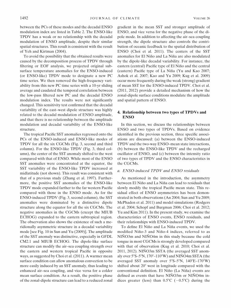
The tropical Pacific SST anomalies regressed onto the
PCs of the ENSO-induced and ENSO-like modes of
TPDV for all the six CGCMs (Fig. 3, second and third
column). For the ENSO-like TPDV (Fig. 3, third col-
umn), the center of the SST anomaly shifted to the west
compared with that of ENSO. While most of the ENSO
SST anomalies were concentrated at the equator, the
SST variability of the ENSO-like TPDV increased at
midlatitude (not shown). This result was consistent with
that of a previous study (Zhang et al. 1997). Further-
more, the positive SST anomalies of the ENSO-like
TPDVmode expanded farther to the far western Pacific
compared with those in the ENSO mode. As for the
ENSO-induced TPDV (Fig. 3, second column), the SST
anomalies were dominated by a distinctive dipole
structure along the equator for all the six CGCMs. The
negative anomalies in the CGCMs (except the MIUB
ECHOG) expanded to the eastern subtropical region.
The observation also shows the existence of such a me-
ridionally asymmetric structure in a decadal variability
mode [see Fig. 10 in Sun and Yu (2009)]. The amplitude
of the SST anomaly was distinctive, especially in GFDL
CM2.1 and MIUB ECHOG. The dipole-like surface
structure can modify the air–sea coupling strength over
the eastern and western tropical Pacific in opposite
ways, as suggested by Choi et al. (2011). A warmer mean
surface condition can allow anomalous convection to be
more easily induced by an SST anomaly, thus leading to
enhanced air–sea coupling, and vice versa for a colder
mean surface condition. As a result, the positive phase
of the zonal-dipole structure can lead to a reduced zonal
gradient in the mean SST and stronger amplitude of
ENSO, and vice versa for the negative phase of the di-
pole mode. In addition to affecting the air–sea coupling
strength, the dipole structure also controls the contri-
bution of oceanic feedback to the spatial distribution of
ENSO (Choi et al. 2011). The centers of the SST
anomalies for El Nino and La Nina are also modulated
by the dipole-like decadal variability. For instance, the
eastern (central) Pacific type of El Nino and the central
(eastern) Pacific type of La Nina (Yu and Kao 2007;
Ashok et al. 2007; Kao and Yu 2009; Kug et al. 2009)
occurmore frequently during the weak (strong) gradient
of mean SST for the ENSO-induced TPDV. Choi et al.
(2011, 2012) provide a detailed mechanism of how the
zonal-dipole surface conditions modulate the amplitude
and spatial pattern of ENSO.
4. Relationship between two types of TPDVs andENSO
In this section, we discuss the relationships between
ENSO and two types of TPDVs. Based on evidence
identified in the previous section, three specific associ-
ations are discussed: (a) between the ENSO-induced
TPDV and the two-way ENSO–mean state interactions,
(b) between the ENSO-like TPDV and the recharged
oscillator of ENSO, and (c) between the intensity ratio
of two types of TPDV and the ENSO characteristics in
the CGCMs.
a. ENSO-induced TPDV and ENSO residuals
As mentioned in the introduction, the asymmetry
between El Nino and La Nina can lead to residuals that
slowly modify the tropical Pacific mean state. This re-
sidual effect of ENSO asymmetries has been demon-
strated in both observations (An 2004; Sun and Yu 2009;
McPhaden et al. 2011) and model simulations (Rodgers
et al. 2004; Schopf and Burgman 2006; Choi et al. 2012;
Yu and Kim 2011). In the present study, we examine the
characteristics of ENSO events, ENSO residuals, and
their relationships with ENSO-induced TPDV.
To define El Nino and La Nina events, we used the
modified Nino-3 and Nino-4 indices, referred to as
NINO3m and NINO4m in this study because the cold
tongue in most CGCMs is strongly developed compared
with that of observation (Kug et al. 2010; Choi et al.
2011, 2012). NINO3m SSTA (the averaged SST anom-
aly over 58S–58N, 1708–1108W) andNINO4m SSTA (the
averaged SST anomaly over 58S–58N, 1408E–1708W)
shifted about 208 west in longitude compared with the
conventional definition. El Nino (La Nina) events are
defined as events that have NINO3m or NINO4m in-
dices greater (less) than 0.58C (20.58C) during the
1492 JOURNAL OF CL IMATE VOLUME 26

boreal winter [D(0)JF(1), where winter is defined as
December–February (DJF)]. Only in the case ofMRI2.3,
normalized NINO3m and NINO4m indices are used
because its ENSO amplitudes are relatively small
compared to those of the other five CGCMs. The
anomalies during El Nino and La Nina winters [D(0)JF
(1)] are composited with respect to the ENSO-induced
TPDV phase. The strong (weak) period is the period
when the normalized PC time series of the ENSO-
induced TPDVyields a standard deviation greater (less)
than 0.5 (20.5). Since ENSO-induced TPDV is highly
correlated with the amplitude modulation of ENSO, the
state of the climate is linked to a strong ENSO period
that corresponds to the positive phase of ENSO-induced
TPDV (Fig. 2, second column). On the other hand, the
state of the climate associated with a weakENSOperiod
is opposite to the pattern expressed in the second col-
umn of Fig. 2.
Residuals induced by the spatial asymmetry between
El Nino and La Nina are calculated by simply adding
El Nino and La Nina composites during boreal winter
[D(0)JF(1)]. Figure 4 shows the residuals induced by
ENSO asymmetries during the strong ENSO period for
the six selected CGCMs. Overall, there is an east–west
contrast pattern similar to the pattern of the ENSO-
induced TPDV. The parentheses shown in each panel
indicate the spatial correlation between the residual
pattern and the EOF pattern of ENSO-induced TPDV.
All CGCMs demonstrate strong similarity in the spatial
pattern, with a correlation coefficient of more than 0.85.
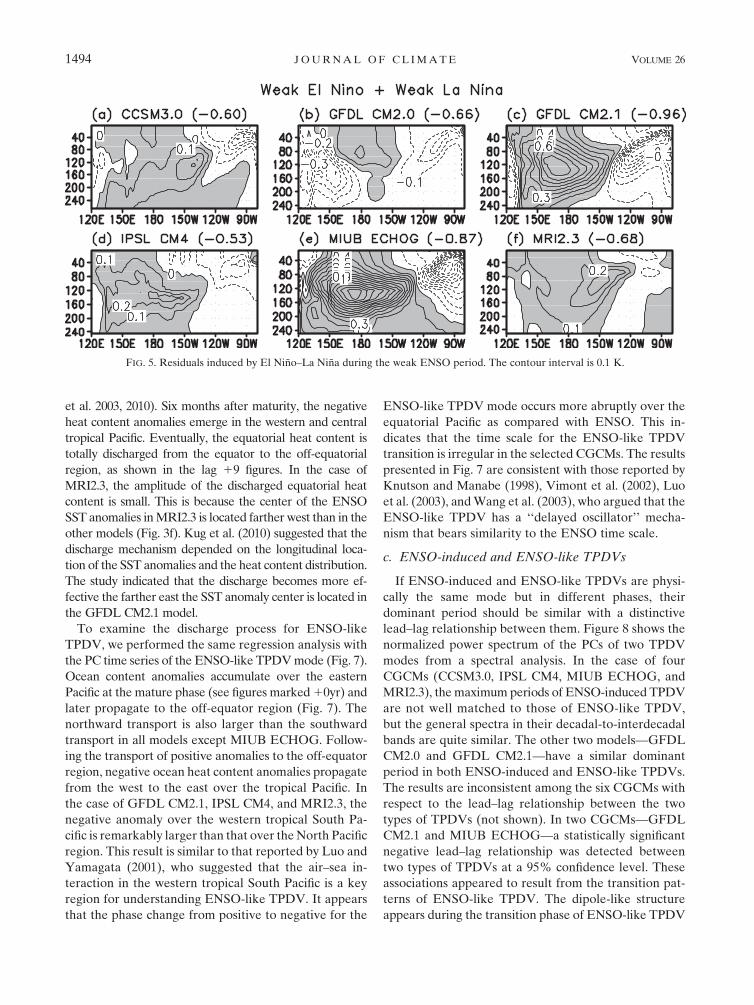
ENSO residuals during the weak ENSO period are
shown in Fig. 5. In the case of GFDL CM2.0, the zonal
dipole structure appears to be collapsed. However,
a general east–west dipole structure also exists in the
other five CGCMs, as demonstrated in Fig. 4, but with
a smaller magnitude. These models also demonstrate
a large negative spatial correlation between ENSO re-
siduals during the weak ENSO period and EOF patterns
of ENSO-induced TPDV.
b. Phase transitions of ENSO-like TPDV and ENSO
According to the recharge oscillator theory, the east-
ward (westward) gradient of heat content conduces
poleward (equatorial) transport bymeridional divergence
(convergence) of the geostrophic currents (Jin 1997a,b;
Meinen andMcPhaden 2001; Kug et al. 2003). The lagged
regression of ocean heat content against the PC time se-
ries of the ENSO mode from the six CGCMs is shown in
Fig. 6. The heat content is defined as the temperature
anomalies vertically integrated from the surface to a depth
of 300 m. The laggedmonths correspond to three, six, and
nine months after the mature phase. Lag 0 represents the
mature phase of the El Nino events. Typically, ocean heat
content anomalies accumulate over the eastern tropical
Pacific during themature phase, threemonths after which
the heat content anomalies start to be transported to
the off-equator region. The northward transport is re-
markably stronger than the southward transport in
four of the CGCMs: CCSM3.0, GFDL CM2.0, GFDL
CM2.1, and IPSL CM4. In the other two models (MIUB
ECHOG and MRI2.3), the northward exchange of heat
content is twice as strong as the southward exchange. This
hemispherically asymmetric discharge process is due to the
southward shift of zonal wind stress from the equator (Kug
FIG. 4. Residuals induced by El Nino–La Nina during the strong ENSO period. The parentheses in the upper right represent the spatial
correlation between the residuals and the EOF pattern of ENSO-induced TPDV. The contour interval is 0.2 K.
1 MARCH 2013 CHO I ET AL . 1493
et al. 2003, 2010). Six months after maturity, the negative
heat content anomalies emerge in the western and central
tropical Pacific. Eventually, the equatorial heat content is
totally discharged from the equator to the off-equatorial
region, as shown in the lag 19 figures. In the case of
MRI2.3, the amplitude of the discharged equatorial heat
content is small. This is because the center of the ENSO
SST anomalies inMRI2.3 is located farther west than in the
other models (Fig. 3f). Kug et al. (2010) suggested that the
discharge mechanism depended on the longitudinal loca-
tion of the SST anomalies and the heat content distribution.
The study indicated that the discharge becomes more ef-
fective the farther east the SST anomaly center is located in
the GFDL CM2.1 model.
To examine the discharge process for ENSO-like
TPDV, we performed the same regression analysis with
the PC time series of the ENSO-like TPDVmode (Fig. 7).
Ocean content anomalies accumulate over the eastern
Pacific at the mature phase (see figures marked10yr) and
later propagate to the off-equator region (Fig. 7). The
northward transport is also larger than the southward
transport in all models except MIUB ECHOG. Follow-
ing the transport of positive anomalies to the off-equator
region, negative ocean heat content anomalies propagate
from the west to the east over the tropical Pacific. In
the case of GFDL CM2.1, IPSL CM4, and MRI2.3, the
negative anomaly over the western tropical South Pa-
cific is remarkably larger than that over theNorth Pacific
region. This result is similar to that reported by Luo and
Yamagata (2001), who suggested that the air–sea in-
teraction in the western tropical South Pacific is a key
region for understanding ENSO-like TPDV. It appears
that the phase change from positive to negative for the
ENSO-like TPDV mode occurs more abruptly over the
equatorial Pacific as compared with ENSO. This in-
dicates that the time scale for the ENSO-like TPDV
transition is irregular in the selected CGCMs. The results
presented in Fig. 7 are consistent with those reported by
Knutson and Manabe (1998), Vimont et al. (2002), Luo
et al. (2003), andWang et al. (2003), who argued that the
ENSO-like TPDV has a ‘‘delayed oscillator’’ mecha-
nism that bears similarity to the ENSO time scale.
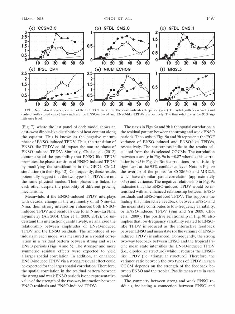
c. ENSO-induced and ENSO-like TPDVs
If ENSO-induced and ENSO-like TPDVs are physi-
cally the same mode but in different phases, their
dominant period should be similar with a distinctive
lead–lag relationship between them. Figure 8 shows the
normalized power spectrum of the PCs of two TPDV
modes from a spectral analysis. In the case of four
CGCMs (CCSM3.0, IPSL CM4, MIUB ECHOG, and
MRI2.3), themaximum periods of ENSO-induced TPDV
are not well matched to those of ENSO-like TPDV,
but the general spectra in their decadal-to-interdecadal
bands are quite similar. The other two models—GFDL
CM2.0 and GFDL CM2.1—have a similar dominant
period in both ENSO-induced and ENSO-like TPDVs.
The results are inconsistent among the six CGCMs with
respect to the lead–lag relationship between the two
types of TPDVs (not shown). In two CGCMs—GFDL
CM2.1 and MIUB ECHOG—a statistically significant
negative lead–lag relationship was detected between
two types of TPDVs at a 95% confidence level. These
associations appeared to result from the transition pat-
terns of ENSO-like TPDV. The dipole-like structure
appears during the transition phase of ENSO-like TPDV
FIG. 5. Residuals induced by El Nino–La Nina during the weak ENSO period. The contour interval is 0.1 K.
1494 JOURNAL OF CL IMATE VOLUME 26
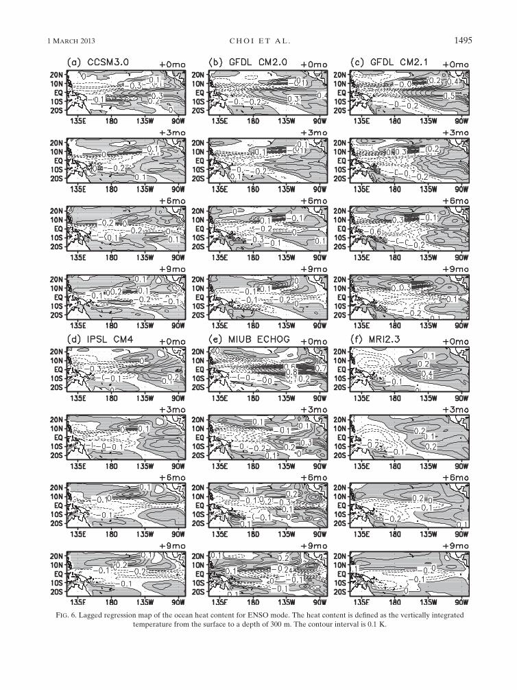
FIG. 6. Lagged regression map of the ocean heat content for ENSO mode. The heat content is defined as the vertically integrated
temperature from the surface to a depth of 300 m. The contour interval is 0.1 K.
1 MARCH 2013 CHO I ET AL . 1495
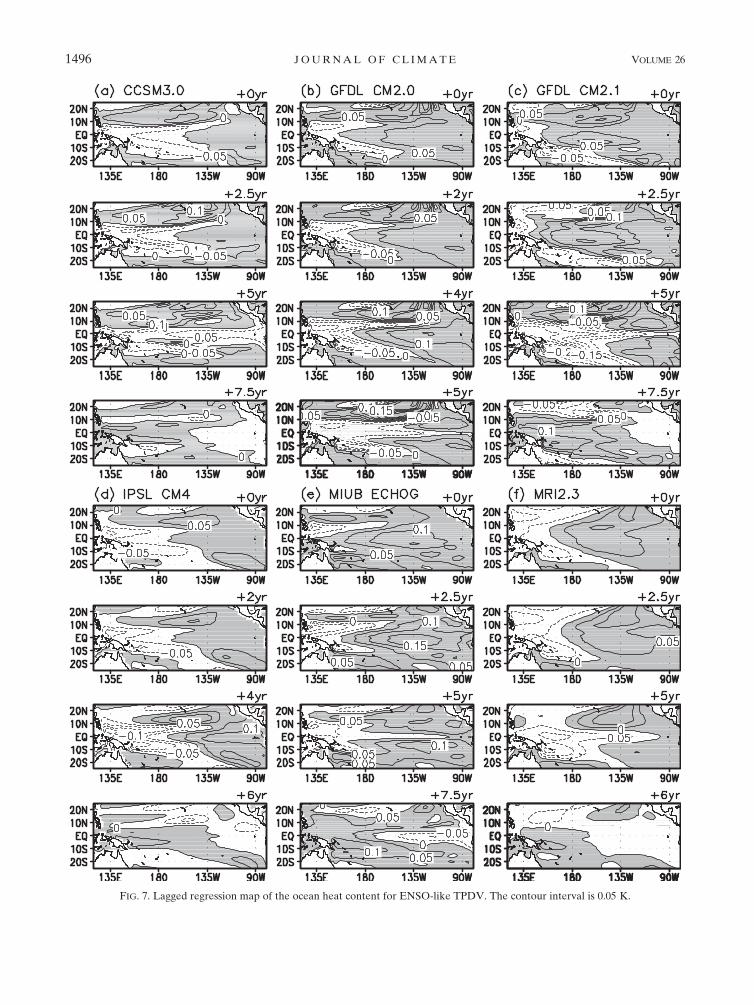
FIG. 7. Lagged regression map of the ocean heat content for ENSO-like TPDV. The contour interval is 0.05 K.
1496 JOURNAL OF CL IMATE VOLUME 26
(Fig. 7), where the last panel of each model shows an
east–west dipole-like distribution of heat content along
the equator. This is known as the negative mature
phase of ENSO-induced TPDV. Thus, the transition of
ENSO-like TPDV could impact the mature phase of
ENSO-induced TPDV. Similarly, Choi et al. (2012)
demonstrated the possibility that ENSO-like TPDV
promotes the phase transition of ENSO-induced TPDV
by modifying the stratification in the GFDL CM2.1
simulation (in their Fig. 12). Consequently, these results
potentially suggest that the two types of TPDVs are not
the same physical modes. Their phases are linked to
each other despite the possibility of different growing
mechanisms.
Meanwhile, if the ENSO-induced TPDV interplays
with decadal change in the asymmetry of El Nino–La
Nina, their strong interaction enhances both ENSO-
induced TPDV and residuals due to El Nino–La Nina
asymmetry (An 2004; Choi et al. 2009, 2012). To un-
derstand this interaction quantitatively, we analyzed the
relationship between amplitudes of ENSO-induced
TPDV and the ENSO residuals. The amplitude of re-
siduals in each model was measured as a spatial corre-
lation in a residual pattern between strong and weak
ENSO periods (Figs. 4 and 5). The stronger and more
symmetric residual effects were expected to yield
a larger spatial correlation. In addition, an enhanced
ENSO-induced TPDV via a strong residual effect could
be expected for the larger spatial correlation. Therefore,
the spatial correlation in the residual pattern between
the strong andweakENSOperiods is one representative
value of the strength of the two-way interaction between
ENSO residuals and ENSO-induced TPDV.
The x axis in Figs. 9a and 9b is the spatial correlation in
the residual pattern between the strong and weak ENSO
periods. The y axis in Figs. 9a and 9b represents the EOF
variance of ENSO-induced and ENSO-like TPDVs,
respectively. The scatterplots indicate the results cal-
culated from the six selected CGCMs. The correlation
between x and y in Fig. 9a is 20.87 whereas this corre-
lation is 0.95 in Fig. 9b. Both correlations are statistically
significant at the 95% confidence level. Note in Fig. 9b
the overlap of the points for CCSM3.0 and MRI2.3,
which have a similar spatial correlation (approximately
0.59) and variance. The negative relationship in Fig. 9a
indicates that the ENSO-induced TPDV would be in-
tensified with an enhanced relationship between ENSO
residuals and ENSO-induced TPDV. This supports the
finding that interactive feedback between ENSO and
the mean state contributes to low-frequency variability,
or ENSO-induced TPDV (Sun and Yu 2009; Choi
et al. 2009). The positive relationship in Fig. 9b also
implies that low-frequency variability related to ENSO-
like TPDV is reduced as the interactive feedback
betweenENSOandmean state (or the variance of ENSO-
induced TPDV) is enhanced. Consequently, the strong
two-way feedback between ENSO and the tropical Pa-
cific mean state intensifies the ENSO-induced TPDV
(i.e., dipole-like structure) while it reduces the ENSO-
like TPDV (i.e., triangular structure). Therefore, the
variance ratio between the two types of TPDV in each
CGCM depends on the strength of the feedback be-
tween ENSO and the tropical Pacific mean state in each
model.
The symmetry between strong and weak ENSO re-
siduals, indicating a connection between ENSO and
FIG. 8. Normalized power spectrum of the EOF PC time series. The x axis indicates the period (year). The solid (with open circle) and
dashed (with closed circle) lines indicate the ENSO-induced and ENSO-like TPDVs, respectively. The thin solid line is the 95% sig-
nificance level.
1 MARCH 2013 CHO I ET AL . 1497
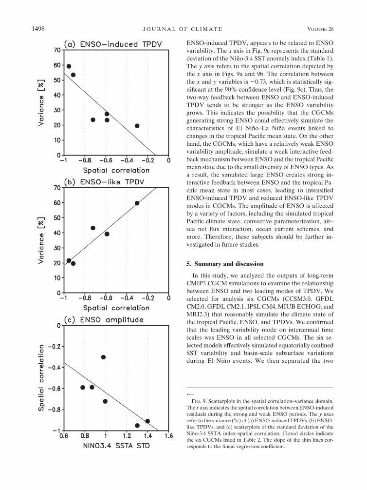
ENSO-induced TPDV, appears to be related to ENSO
variability. The x axis in Fig. 9c represents the standard
deviation of the Nino-3.4 SST anomaly index (Table 1).
The y axis refers to the spatial correlation depicted by
the x axis in Figs. 9a and 9b. The correlation between
the x and y variables is 20.73, which is statistically sig-
nificant at the 90% confidence level (Fig. 9c). Thus, the
two-way feedback between ENSO and ENSO-induced
TPDV tends to be stronger as the ENSO variability
grows. This indicates the possibility that the CGCMs
generating strong ENSO could effectively simulate the
characteristics of El Nino–La Nina events linked to
changes in the tropical Pacific mean state. On the other
hand, the CGCMs, which have a relatively weak ENSO
variability amplitude, simulate a weak interactive feed-
backmechanism between ENSO and the tropical Pacific
mean state due to the small diversity of ENSO types. As
a result, the simulated large ENSO creates strong in-
teractive feedback between ENSO and the tropical Pa-
cific mean state in most cases, leading to intensified
ENSO-induced TPDV and reduced ENSO-like TPDV
modes in CGCMs. The amplitude of ENSO is affected
by a variety of factors, including the simulated tropical
Pacific climate state, convective parameterization, air–
sea net flux interaction, ocean current schemes, and
more. Therefore, these subjects should be further in-
vestigated in future studies.
5. Summary and discussion
In this study, we analyzed the outputs of long-term
CMIP3 CGCM simulations to examine the relationship
between ENSO and two leading modes of TPDV. We
selected for analysis six CGCMs (CCSM3.0. GFDL
CM2.0, GFDLCM2.1, IPSL CM4,MIUBECHOG, and
MRI2.3) that reasonably simulate the climate state of
the tropical Pacific, ENSO, and TPDVs. We confirmed
that the leading variability mode on interannual time
scales was ENSO in all selected CGCMs. The six se-
lected models effectively simulated equatorially confined
SST variability and basin-scale subsurface variations
during El Nino events. We then separated the two
FIG. 9. Scatterplots in the spatial correlation–variance domain.
The x axis indicates the spatial correlation betweenENSO-induced
residuals during the strong and weak ENSO periods. The y axes
refer to the variance (%) of (a) ENSO-induced TPDVs, (b) ENSO-
like TPDVs, and (c) scatterplots of the standard deviation of the
Nino-3.4 SSTA index–spatial correlation. Closed circles indicate
the six CGCMs listed in Table 2. The slope of the thin lines cor-
responds to the linear regression coefficient.
1498 JOURNAL OF CL IMATE VOLUME 26
modes of TPDVby applying an EOF analysis to the low-
pass filtered subsurface temperature anomalies at the
equator. The first mode was the ENSO-induced TPDV,
which is related to the decadal ENSO amplitude mod-
ulation. The PC time series of theENSO-induced TPDV
was highly correlated with the 10-yr sliding standard
deviation of the Nino-3.4 SST anomaly. The spatial
pattern of ENSO-induced TPDV exhibits an east–west
zonal contrast (dipole-like) pattern in its surface and
subsurface structures. The other mode was the ENSO-
like TPDV, which shows a triangular SST structure
similar to ENSO but with a wider meridional extension.
There was a weak relationship between the PC time
series of the ENSO-like TPDV and the decadal modu-
lation index of ENSOamplitude. TheENSO-like TPDV
showed a basin-scale, triangular pattern of SST varia-
tions, but the center of SST anomalies is weaker than the
ENSO and locates farther west. This mode of decadal
variability is characterized by an east–west zonal con-
trast in its subsurface structure, indicating that the ef-
fects of this mode on stratification were increased over
the western tropical Pacific.
With regard to the growth mechanism, the ENSO-
induced TPDV was related to the ENSO residuals
resulting from the spatial asymmetry between El Nino
and La Nina. The asymmetry in El Nino–La Nina
leaves a residual effect in the background state, which
gradually accumulates and gives rise to the ENSO-
induced TPDV. The high simultaneous correlation
between the ENSO-induced TPDV and the decadal
modulation index of ENSO amplitude and the strong
resemblance between the ENSO residual pattern and
the pattern of the ENSO-induced TPDV in the six
CGCMs indicate that these two phenomena strongly
interact with each other. Meanwhile, this interaction
seems to be shown in observation. We note that
McPhaden et al. (2011) addressed the relationship be-
tween the recent more frequent occurrence of central
Pacific El Nino and the changes in the background state,
which is regarded as the negative phase of ENSO-induced
TPDV in this study. On the other hand, a slower recharge/
discharge oscillator works on a decadal-to-interdecadal
time scale, causing ENSO-like TPDV in CGCMs. The
transport of heat content from the equator to the off-
equator follows the peak of ENSO-like TPDV. Mean-
while, the dominant periods of two types of TPDVs are
quite similar even though their growing mechanisms are
different, which appears to be related to the linkage
between their phases. The transition phase of ENSO-
like TPDV has a dipole-like structure at the equator
that is similar to the mature phase of ENSO-induced
TPDV. Therefore, the mature phase of ENSO-induced
TPDV tends to be locked into the transition phase
of ENSO-like TPDV, which could result in similar
periods.
In addition, we compared the variance ratio between
the two types of TPDV in each CGCM and the strength
of interactive feedback between ENSO and the tropical
Pacific mean state. The results support the notion that
these two TPDVs have different growing mechanisms.
When the two-way feedback between ENSO residuals
and ENSO-induced TPDV strengthens, the variance of
the ENSO-induced TPDVwas found to increase but the
variance of the ENSO-like TPDV decreases. The two-
way feedback between ENSO residuals and ENSO-
induced TPDV appears to depend on ENSO variability
in CGCMs.With respect to changes in the tropical Pacific
mean state, the characteristics of El Nino–La Nina were
well simulated when the ENSO variability grew larger
in CGCMs. As a result, the larger ENSO variability in
CGCMs, the stronger interactive feedback between
ENSO and the tropical Pacific mean state leads to an
intensified ENSO-induced TPDV and a weakened
ENSO-like TPDVmode in CGCMs. It should be noted
that this two-way feedback works well for eastern Pa-
cific El Nino than central Pacific El Nino because of its
strong asymmetry (An et al. 2005). In this regard, we
could expect that an increased occurrence of central
Pacific El Nino during the recent decades (Ashok et al.
2007; Yeh et al. 2009) or the relative weakening of
eastern Pacific El Nino variability [this alternation was
argued by Choi et al. (2012)] presumably results in
the intensified ENSO-like TPDV and the weakened
ENSO-induced TPDV. This point needs to be pursued
in the future.
Although we proposed a possible relationship be-
tween ENSO-induced TPDV and ENSO-like TPDV,
particularly a variance ratio between the two TPDVs,
the physical mechanism was not fully addressed in this
study. Furthermore, the basis for the lack of relationship
between ENSO-like TPDV and the decadal ENSO
modulation is not clear, even though the structure of
ENSO-like TPDV is only different on the surface from
ENSO-induced TPDV. Additionally, problems associ-
ated with global warming should be discussed in future
studies. In the future, the ENSO amplitude is likely to
be affected by the changed mean state. Thus, an un-
derstanding of two types of tropical Pacific decadal vari-
ability is essential for improving the predictability of
future ENSO. A more comprehensive study of the phys-
ical linkage between two types of TPDV and sensitivity
tests will be necessary in the near future.
Acknowledgments. This work was funded by the Korea
Meteorological Administration Research and Develop-
ment Program under Grant CATER 2012-3043.
1 MARCH 2013 CHO I ET AL . 1499
REFERENCES
AchutaRao, K. M., and K. R. Sperber, 2002: Simulation of the El
Nino–Southern Oscillation: Results from the Coupled Model
Intercomparison Project. Climate Dyn., 19, 191–209.An, S.-I., 2004: Interdecadal change in the El Nino–La Nina
asymmetry. Geophys. Res. Lett., 31, L23210, doi:10.1029/
2004GL021699.
——, 2009: A review of interdecadal changes in the nonlinearity of
the El Nino–Southern Oscillation. Theor. Appl. Climatol., 97,
29–40.
——, and B. Wang, 2000: Interdecadal change of the structure of
the ENSO mode and its impact on the ENSO frequency.
J. Climate, 13, 2044–2055.
——, Y.-G. Ham, J.-S. Kug, F.-F. Jin, and I.-S. Kang, 2005: El
Nino–La Nina asymmetry in the Coupled Model Inter-
comparison Project simulations. J. Climate, 18, 2617–2627.
——, Z. Ye, andW.W. Hsieh, 2006: Changes in the leading ENSO
modes associated with the late 1970s climate shift: Role of
surface zonal current.Geophys.Res.Lett.,33,L14609, doi:10.1029/
2006GL026604.
Ashok, K., S. K. Behera, S. A. Rao, H. Weng, and T. Yamagata,
2007: El NinoModoki and its teleconnection. J. Geophys. Res.,
112, C11007, doi:10.1029/2006JC003798.
Bejarano, L., and F.-F. Jin, 2008: Coexistence of equatorial coupled
modes of ENSO. J. Climate, 21, 3051–3067.
Burgman, R. J., P. S. Schopf, and B. P. Kirtman, 2008: Decadal
modulation of ENSO in a hybrid coupled model. J. Climate,
21, 5482–5500.Carton, J. A., and B. S. Giese, 2008: A reanalysis of ocean cli-
mate using Simple Ocean Data Assimilation (SODA).Mon.
Wea. Rev., 136, 2999–3017.
——,——, and S. A. Grodsky, 2005: Sea level rise and the warming
of the oceans in the SimpleOceanDataAssimilation (SODA)
ocean reanalysis. J. Geophys. Res., 110, C09006, doi:10.1029/
2004JC002817.
Choi, J., S.-I. An, B. Dewitte, and W. W. Hsieh, 2009: Interactive
feedback between the tropical Pacific decadal oscillation and
ENSO in a coupled general circulation model. J. Climate, 22,
6597–6611.
——, ——, J.-S. Kug, and S.-W. Yeh, 2011: The role of mean state
on changes in El Nino’s flavor. Climate Dyn., 37, 1205–1215.
——,——, and S.-W. Yeh, 2012: Decadal amplitudemodulation of
two types of ENSO and its relationship with the mean state.
Climate Dyn., 38, 2631–2644.Cibot, C., E. Maisonnave, L. Terray, and B. Dewitte, 2005: Mech-
anisms of tropical Pacific interannual-to-decadal variability in
the ARPEGE/ORCA global coupled model. Climate Dyn., 24,
823–842.
Collins, M., and Coauthors, 2010: The impact of global warming on
the tropical Pacific Ocean and El Nino. Nat. Geosci., 3, 391–
397.
Dewitte, B., S.-W. Yeh, B.-K. Moon, C. Cibot, and L. Terray, 2007:
Rectification of the ENSO variability by interdecadal changes
in the equatorial background mean state in a CGCM simula-
tion. J. Climate, 20, 2002–2021.
——, S. Thual, S.-W. Yeh, S.-I. An, B.-K. Moon, and B. S. Giese,
2009: Low-frequency variability of temperature in the vicinity
of the equatorial Pacific thermocline in SODA: Role of
equatorial wave dynamics and ENSO asymmetry. J. Climate,
22, 5783–5795.
Evans, M. N., A. Kaplan, and M. A. Cane, 2002: Pacific sea surface
temperature field reconstruction from coral d18O data using
reduced space objective analysis. Paleoceanography, 17, 1007,
doi:10.1029/2000PA000590.
Fedorov, A. V., and S. G. H. Philander, 2000: Is El Nino changing?
Science, 288, 1997–2002.
——, and ——, 2001: A stability analysis of tropical ocean–
atmosphere interactions: Bridging measurements and theory
for El Nino. J. Climate, 14, 3086–3101.
Flugel, M., and P. Chang, 1999: Stochastically induced climate shift
of El Nino–Southern Oscillation. Geophys. Res. Lett., 26,
2473–2476.
Garreaud, R., and D. S. Battisti, 1999: Interannual (ENSO) and
interdecadal (ENSO-like) variability in the Southern Hemi-
sphere tropospheric circulation. J. Climate, 12, 2113–2123.
Hannachi, A., D. Stephenson, and K. Sperber, 2003: Probability-
based methods for quantifying nonlinearity in the ENSO.
Climate Dyn., 20, 241–256.
Imada, Y., and M. Kimoto, 2009: ENSO amplitude modulation
related to Pacific decadal variability. Geophys. Res. Lett., 36,
L03706, doi:10.1029/2008GL036421.
Jin, F.-F., 1997a: An equatorial ocean recharge paradigm for
ENSO. Part I: Conceptual model. J. Atmos. Sci., 54, 811–
829.
——, 1997b: An equatorial ocean recharge paradigm for ENSO.
Part II: A stripped-down coupled model. J. Atmos. Sci., 54,
830–847.
——, J. D. Neelin, and M. Ghil, 1994: El Nino on the devil’s
staircase: Annual subharmonic steps to chaos. Science, 264,
70–72.
Kao, H. Y., and J.-Y. Yu, 2009: Contrasting eastern-Pacific and
central-Pacific types of ENSO. J. Climate, 22, 615–632.Kirtman, B. P., and P. S. Schopf, 1998: Decadal variability in ENSO
predictability and prediction. J. Climate, 11, 2804–2822.
Knutson, T. R., and S. Manabe, 1998: Model assessment of decadal
variability and trends in the tropical Pacific Ocean. J. Climate,
11, 2273–2296.Kug, J.-S., I.-S. Kang, and S.-I. An, 2003: Symmetric and anti-
symmetric mass exchanges between the equatorial and off-
equatorial Pacific associated with ENSO. J. Geophys. Res.,
108, 3284, doi:10.1029/2002JC001671.
——, F.-F. Jin, and S.-I. An, 2009: Two types of El Nino events:
Cold tongue El Nino and warm pool El Nino. J. Climate, 22,
1499–1515.
——, J. Choi, S.-I. An, F.-F. Jin, and A. T.Wittenberg, 2010:Warm
pool and cold tongue El Nino events as simulated by the
GFDL 2.1 coupled GCM. J. Climate, 23, 1226–1239.
Latif, M., R. Kleeman, and C. Eckert, 1997: Greenhouse warming,
decadal variability, or El Nino? An attempt to understand the
anomalous 1990s. J. Climate, 10, 2221–2239.
——, and Coauthors, 2001: ENSIP: The El Nino simulation in-
tercomparison project. Climate Dyn., 18, 255–276.
Li, J., and Coauthors, 2011: Interdecadal modulation of El Nino
amplitude during the past millennium.Nature Climate Change,
1, 114–118.Luo, J.-J., and T. Yamagata, 2001: Long-term El Nino–Southern
Oscillation (ENSO)-like variation with special emphasis on
the South Pacific. J. Geophys. Res., 106 (C10), 22 211–22 227.
——, S. Masson, S. Behera, P. Delecluse, S. Gualdi, A. Navarra,
and T. Yamagata, 2003: South Pacific origin of the decadal
ENSO-like variation as simulated by a coupled GCM. Geo-
phys. Res. Lett., 30, 2250, doi:10.1029/2003GL018649.
Mantua, N. J., S. R. Hare, Y. Zhang, J. M. Wallace, and R. C.
Francis, 1997: A Pacific decadal climate oscillationwith impacts
on salmon production.Bull. Amer. Meteor. Soc., 78, 1069–1079.
1500 JOURNAL OF CL IMATE VOLUME 26

McPhaden, M. J., T. Lee, and D. McClurg, 2011: El Nino and its
relationship to changing background conditions in the tropical
Pacific Ocean. Geophys. Res. Lett., 38, L15709, doi:10.1029/
2011GL048275.
Meehl, G. A., C. Covey, K. E. Taylor, T. Delworth, R. J. Stouffer,
M. Latif, B. McAvaney, and J. F. B. Mitchell, 2007: The
WCRP CMIP3 multimodel dataset: A new era in climate
change research. Bull. Amer. Meteor. Soc., 88, 1383–1394.Meinen, C. S., andM. J.McPhaden, 2001: Interannual variability in
warm water volume transports in the equatorial Pacific during
1993–99. J. Phys. Oceanogr., 31, 1324–1345.
Rodgers, K. B., P. Friederichs, and M. Latif, 2004: Tropical Pacific
decadal variability and its relation to decadal modulations of
ENSO. J. Climate, 17, 3761–3774.
Schopf, P. S., and R. J. Burgman, 2006: A simple mechanism for
ENSO residuals and asymmetry. J. Climate, 19, 3167–3179.
Sun, F., and J.-Y. Yu, 2009: A 10–15-yr modulation cycle of ENSO
intensity. J. Climate, 22, 1718–1735.
Sverdrup, H. U., M. W. Johnson, and R. H. Fleming, 1942: The
Oceans: Their Physics, Chemistry, and General Biology.
Prentice-Hall, 1087 pp.
Thual, S., B. Dewitte, S.-I. An, and N. Ayoub, 2011: Sensitivity of
ENSO to stratification in a recharge–discharge conceptual
model. J. Climate, 24, 4332–4349.
Timmermann, A., 2003: Decadal ENSO amplitude modulations: A
nonlinear paradigm. Global Planet. Change, 37, 135–156.——, J. Oberhuber, A. Bacher, M. Esch, M. Latif, and E. Roeckner,
1999: Increased El Nino frequency in a climate model forced
by future greenhouse warming. Nature, 398, 694–697.
Vimont, D. J., D. S. Battisti, and A. C. Hirst, 2002: Pacific in-
terannual and interdecadal equatorial variability in a 1000-yr
simulation of the CSIRO coupled general circulation model.
J. Climate, 15, 160–178.Wallace, J. M., and D. S. Gutzler, 1981: Teleconnections in the
geopotential height field during the Northern Hemisphere
winter. Mon. Wea. Rev., 109, 784–812.
Wang, X., F.-F. Jin, and Y. Wang, 2003: A tropical ocean recharge
mechanism for climate variability. Part II: A unified theory for
decadal and ENSO modes. J. Climate, 16, 3599–3616.
Yeh, S.-W., and B. Kirtman, 2004: Tropical Pacific decadal vari-
ability and ENSO amplitude modulation in a CGCM. J. Geo-
phys. Res., 109, C11009, doi:10.1029/2004JC002442.
——, J.-S. Kug, B. Dewitte,M.-H. Kwon, B. Kirtman, and F.-F. Jin,
2009: El Nino in a changing climate. Nature, 461, 511–514;Corrigendum, 462, 674.
Yu, B., and G. J. Boer, 2004: The role of the western Pacific in
decadal variability.Geophys. Res. Lett., 31, L02204, doi:10.1029/
2003GL01847.
Yu, J.-Y., and H.-Y. Kao, 2007: Decadal changes of ENSO persis-
tence barrier in SST and ocean heat content indices: 1958–2001.
J. Geophys. Res., 112, D13106, doi:10.1029/2006JD007654.
——, and S. T. Kim, 2011: Reversed spatial asymmetries between
El Nino and La Nina and their linkage to decadal ENSO
modulation in CMIP3 models. J. Climate, 24, 5423–5434.
Zebiak, S. E., 1989: On the 30-60 day oscillation and the prediction
of El Nino. J. Climate, 2, 1381–1387.
Zhang, Y., J. M. Wallace, and D. S. Battisti, 1997: ENSO-like in-
terdecadal variability: 1900–93. J. Climate, 10, 1004–1020.
1 MARCH 2013 CHO I ET AL . 1501