Impacts of pre-existing ocean cyclonic circulation on sea surface Chlorophyll-a concentrations off northeastern Taiwan following episodic typhoon passages Fang-Hua Xu1,* ,Yao Yuan1, Leo Oey2,3 , Yanluan Lin1
1. Ministry of Education Key Laboratory for Earth System Modeling, and Department of
Earth System Science, Tsinghua University, Beijing, China
2. Program in Atmospheric and Oceanic Sciences, Princeton University, Princeton, USA
3. National Central University, Zhongli, Taiwan
*Corresponding author: [email protected]
June 2017 Submitted to Journal of Geophysical Research: Oceans
Keywords: cyclonic eddies, chlorophyll, typhoon, Kuroshio, off northeastern Taiwan Key points 1. Off northeastern Taiwan, enhancement of sea surface chlorophyll-a concentration is frequently found after typhoon passage. 2. A pre-existing ocean cyclonic circulation tends to be intensified and promote strong upwelling and phytoplankton growth after a typhoon. 3. Dynamical interpretations of the cyclone intensification induced by typhoons are proposed.
Research Article Journal of Geophysical Research: OceansDOI 10.1002/2016JC012625
This article has been accepted for publication and undergone full peer review but has not beenthrough the copyediting, typesetting, pagination and proofreading process which may lead todifferences between this version and the Version of Record. Please cite this article asdoi: 10.1002/2016JC012625
© 2017 American Geophysical UnionReceived: Dec 14, 2016; Revised: Jun 01, 2017; Accepted: Jul 05, 2017
This article is protected by copyright. All rights reserved.

2
Abstract Off northeastern Taiwan, enhancement of sea surface chlorophyll-a (Chl-a)
concentration is frequently found after typhoon passages. From 1998 to 2013, forty-six typhoon events are analyzed to examine the variations in Chl-a concentration from satellite ocean color data. On average, Chl-a concentration increased by 38% after a typhoon passage. Noticeably, four remarkable Chl-a increases after typhoons coincide with pre-existing oceanic cyclones in the study area. The Chl-a increase is significantly anti-correlated (p<0.01) with relative SSH, defined as the difference of SSH in the study area and in the surrounding area. To assess the impact of pre-existing cyclones on the upper ocean response to typhoons, we conduct a series of numerical experiments to simulate the oceanic response to Typhoon Kaemi (2006) with or without a pre-existing oceanic cyclone, and with or without strong typhoon winds. The results show that the experiment with a pre-existing oceanic cyclone produces the largest upwelling due to cyclone intensification, mainly induced by the positive wind stress curl dipole northeast of Taiwan.
This article is protected by copyright. All rights reserved.

3
1. Introduction
The influences of tropical cyclones or typhoons/hurricanes on ecosystem over
continental shelves and open oceans have been documented worldwide (e.g. Chen et
al. 2003; Lin 2012; Hung et al. 2013; Foltz et al. 2015; Huang and Oey 2015; Lin and
Oey 2016). After typhoon passages, increases of sea surface chlorophyll-a (Chl-a)
concentration are often found. In coastal regions, typhoon-induced mixing, enhanced
terrestrial runoff, and resuspension are considered as the three major processes that
contribute to the increased nutrient concentrations and subsequent primary production
in the euphotic layer (Chen et al. 2003). In open oceans, phytoplankton blooms were
sometimes observed after typhoon passages (e.g. Shang et al. 2008; Lin 2012; Foltz et
al. 2015). Ocean re-stratification after mixing and entrainment of subsurface nutrients
by typhoon passages is one of the key mechanisms for the subsequent blooms (Huang
and Oey, 2015; Lin and Oey 2016).
Off northeastern Taiwan, the enhancement of Chl-a concentration is frequently
found following episodic typhoon passages across the shelf of the East China Sea (e.g.
Chang et al. 2008; Siswanto et al. 2009; Chang et al. 2014). It is mainly attributed to
increased nutrient supply to the euphotic zone induced by vertical mixing/entrainment,
upwelling, and Kuroshio subsurface water intrusion associated with typhoons (e.g.
Siswanto et al. 2009;Morimoto et al. 2009; Liu et al. 2015). For example, Hung et al.
(2013) observed significant nutrient supply caused by strong upwelling and/or vertical
mixing after Typhoon Morakot (2009). Previous studies in the area have identified
This article is protected by copyright. All rights reserved.

4
typhoon intensity, translation speed, and Kuroshio axis shifts are important factors influencing the upper ocean responses to typhoons (e.g. Chang et al, 2008; Siswanto al. 2009; Shibano et al. 2011; Shan et al. 2014; Zhao et al. 2015). Another important factor may be the excessive river outflows by rainfall associated with typhoons, which enhances buoyancy effects, and then facilitates the onshore transport of nutrient-rich subsurface Kuroshio waters (Chen et al. 2003).
It is noteworthy that a cold dome or cyclonic circulation, approximately 100 km in diameter, often appears just northeast of Taiwan during summer and fall (e.g. Wu et al. 2008; Jan et al. 2011; Gopalakrishnan et al. 2013). Having lower temperature and higher salinity than ambient waters, it is centered near 122.125oE, 25.625oN (Jan et al. 2011), and lasts for one or two weeks (Gopalakrishnan et al. 2013). The formation of the cold dome has been connected with the seasonal variability of Kuroshio migration and transport (Wu et al. 2008; Shen et al. 2011; Gopalakrishnan et al. 2013).
The responses of pre-existing ocean cyclonic circulations to tropical cyclones have been explored in several studies. Walker et al. (2005) found rapid intensification of a cyclonic eddy with phytoplankton blooms 3-4 days after the passage of Hurricane Ivan in the Gulf of Mexico. Zheng et al. (2008) revealed that the intensive cooling following a typhoon passage was induced by pre-existing cyclonic flow and uplifted thermocline in the North Pacific. Zheng et al. (2010) found pre-existing cyclonic significantly enhance upper ocean cooling in response to strong typhoons in the western North Pacific. Chen and Tang (2012) reported the formation of a
This article is protected by copyright. All rights reserved.

5
phytoplankton bloom associated with a cyclonic eddy after tropical cyclone Linfa (2009) over the northern South China Sea. Off northeastern Taiwan, the passage of Typhoon Haitang (2005) and Typhoon Morakot (2009) were found to intensify the pre-existing cold domes (Chang et al. 2008; Morimoto et al. 2009; Jan et al. 2011). et al. (2011) discussed possible physical responses of cold domes to typhoons. intrusion of Kuroshio waters is generated by the northeasterly-northerly wind during the first half of typhoon passages. Upwelling of nutrient-rich Kuroshio subsurface water is then induced by the southerly-southwesterly wind during the second half of typhoon passages. As a consequence, the primary production or Chl-a concentrations are enhanced in the cold dome area. Because of the strong shear of the Kuroshio, what roles pre-existing cyclonic circulation and Kuroshio play in response to typhoon passage northeast of Taiwan need further investigation.
In this study, we revisit upper ocean responses to typhoons off northeastern Taiwan, focusing on the role of the pre-existing ocean conditions on Chl-a enhancement. Long-term satellite observations of sea surface Chl-a concentration, sea
surface temperature (SST), surface wind, and ocean reanalysis data are analyzed first.
Then, typhoon Kaemi (2006) is taken as an example to explore the effects of a
persisting oceanic cyclone on the upwelling and entrainment in the area via a series of
numerical experiments. Section 2 describes the data and model used. Section 3
discusses the effects of typhoons and oceanic conditions on sea surface Chl-a
concentrations from long-term data analysis. Section 4 compares the results of the
This article is protected by copyright. All rights reserved.

6
numerical experiments under various ocean conditions and wind strengths. Dynamical
interpretations of the cyclone intensification induced by typhoons are proposed.
Conclusions and discussion are given in Section 5.
2. Data and numerical experiments
2.1 Data
Typhoon best track, minimum sea level pressure, and maximum wind speed data
are obtained from International Best Track Archive for Climate Stewardship
(IBTrACS, Knapp et al. 2010). The IBTrACS data are later used in the vortex model
of Holland (1980) to estimate typhoon winds for numerical experiments.
Daily sea surface Chl-a concentrations at 9-km resolution were obtained from the
Sea-viewing Wide Field-of-view Sensor (SeaWiFS) from 1998-2010
(http://oceancolor.gsfc.nasa.gov/SeaWiFS/) and the two Moderate Resolution Imaging
Spectroradiometers (MODIS) on Aqua and Terra from 2000-2013
(http://modis.gsfc.nasa.gov/data/dataprod/chlor_a.php).
In order to explore the upper ocean response to typhoon events, we investigate
surface height (SSH), sea surface temperature (SST), surface wind vectors, and
Kuroshio intrusion in the study region from 1998 to 2013. The daily 0.25o×0.25o
gridded SSH is obtained from AVISO (http://www.aviso.oceanobs.com). SST is from
the multi-channel Advanced Very High Resolution Radiometer (AVHRR,
http://gcmd.nasa.gov/records/GCMD_NAVOCEANO_MCSST.html). Sea surface
wind vectors are from the six-hourly cross-calibrated multi-platform wind (CCMP,
This article is protected by copyright. All rights reserved.
7
Atlas et al. 2011). The global 1/12o reanalysis data from HYbrid Coordinate Ocean
Model with Navy Coupled Ocean Data Assimilation (HYCOM+NCODA,
http://hycom.org/dataserver/glb-reanalysis, Cummings and Smedstad, 2013) is used to
estimate the transport of Kuroshio cross-shore intrusion. AVISO along-track SSH,
satellite SST observations, in-situ measurements of temperature from XBTs, and
temperature and salinity profiles from Argo floats and moorings are assimilated in the
system. The reanalysis data has been extensively verified and widely used in global
oceans and shelf regions, including northeast of Taiwan to study Kuroshio intrusion
variability (Yin et al., 2017).
2.2 Numerical experiments
We use the North Pacific Ocean model of Advanced Taiwan Ocean Prediction
system (ATOP, Oey et al. 2013; Sun et al. 2015) to simulate the ocean response to
typhoon Kaemi (2006). The model is developed from the parallel version of the
Princeton Ocean Model (POM). It is configured for the North Pacific from
99°E-70°W and 15°S-72°N at 0.1° × 0.1° horizontal resolution and 41 vertical sigma
levels, with realistic topography based on the ETOPO2. ETOPO2 has a 2-minute
resolution (https://www.ngdc.noaa.gov/mgg/fliers/01mgg04.html). Details about the
model physics are referred to Oey et al. (2013). The model has been used to study
ocean and typhoon interactions over the South China Sea (e.g. Sun et al. 2015), as
well as in studies of typhoon-induced chlorophyll blooming [Huang and Oey 2015;
Lin and Oey 2016].
This article is protected by copyright. All rights reserved.

8
To investigate the impact of pre-existing cyclonic circulation on upper ocean
response to typhoons, we conduct three numerical experiments (Table 1). Experiment
1 has both the passage of Typhoon Kaemi (2006) and pre-existing cyclonic circulation.
It is initialized on July 15th, one week before typhoon arrival. The initial conditions
are produced by ATOP data assimilation system (details are given in Oey et al. 2013
and Xu and Oey 2014, 2015). Note that the strength of CCMP winds is much weaker
than that of the real typhoon winds near the eyewall by as much as 50% (Sun et al.
2015). The typhoon winds are therefore generated from the vortex model of Holland
(1980) based on the minimum sea level pressure and maximum wind speed of Kaemi
(2006) from IBTrACS [Oey and Chou 2016]. The vortex winds are merged with the
CCMP wind using a Gaussian weight with an e-folding decay radius of 350 km, such
that there was a smooth transition from the vortex model to CCMP winds at distance
far away from the typhoon center (Fig. S1). Noticeably the wind is enhanced over
both ocean and land in the vortex model, but the influence of strong wind over land
cannot impact the ocean model response. Experiment 2 has the same typhoon winds
but without the pre-existing ocean cyclone. It is initialized at an earlier date, July 6th
when there was no ocean cyclone off northeastern Taiwan (Fig. S2). Experiment 3 has
the same pre-existing oceanic conditions as Experiment 1 but using the weaker winds
from CCMP.
3. Statistical analysis of oceanic response to typhoon events
Forty-six typhoon passages around Taiwan Island are analyzed between 1998
This article is protected by copyright. All rights reserved.

9
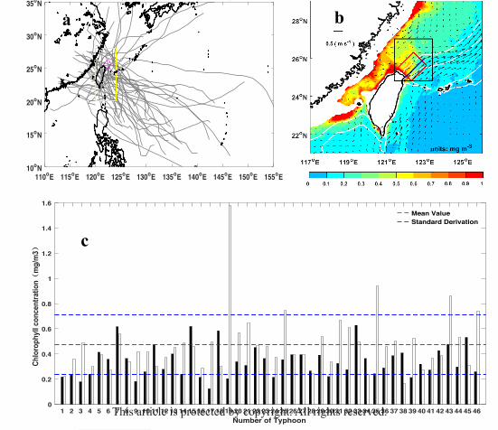
2013 for which satellite Chl-a data is available (Fig.1a). The name and landing time of
the 46 typhoons are listed in Table S1. The 8-day averaged Chl-a concentrations after
typhoon passages are shown in Figure 1b. The 8 days are counted after the time when
distance from a typhoon center to the study area is the shortest. Over the continental
shelf, the Chl-a concentration is large due to the enhanced river runoff, mixing,
resuspension, and so on. Off northeastern Taiwan, the Chl-a is large as well over the
continental shelf break. The red box, centered at 122.35oE, 25.55oN, denotes our study
area, and the black box (24.8o-27oN, 121.4o-123.4oE,) denotes the ambient
The surface appearance of the cyclonic circulation or cold dome can be inferred from
the differences of mean AVISO SSH between the red box and the black box, named
relative SSH (RSSH, hereafter). The red box SSH is masked out when computing the
black box mean SSH. Negative values indicate the appearance of cyclonic circulations,
while positive values correspond to anticyclones.
Figure 1c compares the 5-day averaged Chl-a concentration before typhoon
and 8-day averaged Chl-a concentration after typhoon passage. 5-day average before
typhoon is used to represent proximate pre-typhoon ocean conditions. While 8-day
averaged Chl-a after typhoon is used to reduce satellite data gaps due to cloudy
conditions and retain the bloom signal caused by typhoon (Siswanto et al. 2009).
Before typhoon arrival, the averaged Chl-a concentration of 46 events was about 0.34
mg m-3, while after typhoon passage, the concentration increased to about 0.47 mg m-3.
The averaged increase of Chl-a was approximately 38%. The background standard
This article is protected by copyright. All rights reserved.

10
deviation of Chl-a (excluding 8-day Chl-a concentration after typhoons) is about 0.32
mg m-3. Including the 8-day Chl-a concentration, the standard deviation becomes
0.37 mg m-3. The perturbation induced by typhoons increases Chl-a variability.
Enhancement of Chl-a concentration was found following 32 typhoon events.
of Chl-a appeared after 14 typhoons. Their tracks and intensities are shown in Figure
The reasons for CHL decrease are diverse. Note that most typhoon intensities are
(<33 m s-1) close to the study area, except No. 33, No 34 and No. 38. For typhoon No.
6, 7, 8, 28 and 40, the decrease is less than 5% of their original Chl-a concentration.
Previous typhoons, which had already stimulated blooms, would impair the ocean
response to the adjacent following typhoons (e.g. No.15, 28, 38, &45). The other
might be the preferred mixing on the right side of typhoon tracks (Price 1981; Huang
and Oey 2015). So if the study area is on the left side of typhoons (e.g. No. 7, 18,
it is unfavorable for mixing. The vorticity analysis, discussed in the study (details in
Section 4.3), suggests that typhoons passing through the study area or further
north/northeastward (e.g. No. 5, 7, 8, 11, 33, 34&42) tend to produce unfavorable
upwelling conditions. Besides moving directions, the typhoon translation speed, size,
and the first order baroclinic phase speed tend to influence the mixing and upwelling
well, as suggested by Sun et al. (2015).
There are 5 typhoons that stimulate phytoplankton blooms exceeding +1
deviation (0.22 mg m-3) of Chl-a concentration (Fig. 1c), No.19 Typhoon Haitang
(2005), No.25 Kaemi (2006), No. 35 Morakot (2009), No. 43 Soulik (2013), and No.
This article is protected by copyright. All rights reserved.

11
Usagi (2013). After checking the AVISO SSH, we found 4 of these 5 typhoons have
pre-existing cyclonic circulations in the bloom area except Typhoon Soulik (2013),
implying the importance of the pre-existing cyclonic circulations on enhancement of
Chl-a after typhoon passage. The spatial distributions of Chl-a concentration after the
four typhoon passages are shown in Figure S4. It is consistent with previous findings
for Typhoon Haitang (2005) by Chang et al. (2008) and Typhoon Morakot (2009) by
Morimoto et al. (2009) and Hung et al. (2013).
To explore the impact of pre-existing oceanic conditions on Chl-a, we regress
the differences of Chl-a concentration after and before typhoon passage onto RSSH
(Fig. 2a). The time when distance from a typhoon center to the study area is the
shortest is used to separate the passage of the typhoon. The regression coefficient is
about -0.06 mg m-3 cm-1, and the correlation coefficient is about -0.49, significant at
the 99% confidence level (p<0.01). This suggests that the lower RSSH favors larger
Chl-a increase. The aforementioned 4 typhoons all created relatively large increases in
Chl-a. Note that the shelf SSH tends to be higher when the typhoon is still quite far away – i.e. 1 day away (or ~400 km from northeast Taiwan for mean TC translation speed of about 5m/s), so the low RSSH may partly due to the higher shelf SSH (black box in Fig.1b) induced by the northeasterly wind that often precedes the typhoon. That may explain the large scatter in Figure 2a. To better understand the effects of Kuroshio intrusion on Chl-a, we calculate the
7-day averaged Kuroshio transport onto the shelf region using HYCOM+NCODA
This article is protected by copyright. All rights reserved.

12
during typhoon passage. The onshore Kuroshio transport is integrated along the section (the blue line in Fig. 1b) from bottom to surface. The velocities from are rotated to be normal to the blue line for the transport calculation. Yin et al.
(2017) showed a good agreement between the HYCOM reanalysis data and AVISO
geostrophic currents, and drifter trajectories from Global Drifter Program northeastern
of Taiwan (see their Figs. 2&3). Both onshore (positive) and offshore (negative)
transports are found. The correlation coefficient is only about 0.21 and not significant
(p>0.05). Because Kuroshio onshore and offshore intrusions vary with typhoon
passages and pre-existing oceanic conditions, the effects of Kuroshio on Chl-a
concentration remain unclear. Different typhoons tend to induce different Kuroshio
intrusion strength. It suggests that a numerical simulation of Kuroshio is necessary to
better understand the responses of a pre-existing oceanic cyclone and associated
Kuroshio to a typhoon.
4. Oceanic response to Typhoon Kaemi (2006) using numerical experiments
To better understand the effects of Kuroshio intrusion and a pre-existing oceanic
cyclone on Chl-a, we use Typhoon Kaemi (2006; see its track in Fig. 3a) as an
to study the ocean responses to typhoons. It is one of the five typhoons that stimulate
phytoplankton blooms exceeding +1 standard deviation of Chl-a (No.25 from Fig. 1b).
Kaemi (2006) was formed about 1600 km east of central Philippines on July 19, 2006
as a low-pressure system. Later on, it moved northwestward and developed into a
typhoon. It first landed at Taiwan Island at 1550 UTC July 24 with a maximum wind
This article is protected by copyright. All rights reserved.

13
speed exceeding 50 m s-1. The typhoon entered the Taiwan Strait at 2000 UTC July 24
with the maximum wind speed of 33 m s-1, landed again and became a tropical
depression in Fujian Province of China at 2100 UTC, July 25. Finally, it dissipated on
July 26. Figure 3a showed the distribution of 8-day averaged Chl-a concentration after
the typhoon passage. Off northeastern Taiwan, a phytoplankton bloom appeared.
Meanwhile, a cyclone was seen and intensified during typhoon passage from AVISO
SSH (Fig. 3b). This case provides us a good example to better understand the
of a pre-existing cyclone and the Kuroshio in the area to typhoons.
We conducted three numerical experiments to explore the upper ocean response
to Typhoon Kaemi (Table 1). For the three experiments, the variations in SSH and
surface currents were compared first. Then, vertical sections of temperature and
salinity were compared to detect the upper ocean response. Variations in vertical
velocity (w) were further investigated because it was one of the main factors that
bring nutrients to the upper layer. Intense vertical mixing induced by typhoons is
another main contributor to enhanced nutrient supply in the upper ocean (e.g. Chiang
et al. 2011; Huang and Oey 2015). The variations in the vertical mixing are discussed
as well. 4.1 Evolution of the pre-existing cyclone
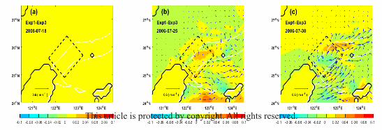
The evolution of the upper ocean state for the three experiments differs markedly.
Figure 4 compares the SSH and surface velocities from the three experiments before
(Jul. 18), during (Jul. 25) and after (Jul. 30) typhoon passage. On July 18th before
Typhoon arrival, a weak cyclonic circulation appears off northeastern Taiwan,
This article is protected by copyright. All rights reserved.

14
at about 25.7oN and 122.2oE for Exp.1 and Exp.3. The strengths of cyclones are the
same for the two experiments because of the same initial conditions. As designed,
is no cyclonic circulation for Exp.2. Besides, the location of Kuroshio in Exp.2 is
onshore than the other two cases.
When the typhoon passes by on July 25th, a stronger cyclonic circulation was
developed in Exp.1 than Exp.3 (Fig. 4b, h). The differences of SSH and surface
currents between Exp. 1 and Exp. 3 are shown in Figure 5. The locations of the
cyclone and Kuroshio are consistent with those inferred from AVISO SSH (Fig. 3
right). On July 30th, there still exists a clear cyclone after the dissipation of typhoon
Kaemi in Exp. 1 and Exp. 3 (Fig. 4c&i). A stronger cyclone develops in Exp. 1 than in
Exp. 3. Again, no cyclone appears for Exp. 2.
4.2 Upper ocean responses to the typhoon passage
The vertical sections of salinity and temperature along 25.5oN are shown in
6 and 7, respectively. On July 18th, the salinity west of 122oE above 100 m is relative
low (<34.6 psu), and salinity maximum (>34.8 psu) of the North Pacific Tropical
(NPTW) is found between 50 m and 200 m depth for Exp. 1 and Exp. 3. Isohalines
(34.6 psu) around 122oE below 200 m are uplifted due to the existence of a cyclone.
contrast, low salinity water appears approximately below 300 m for Exp. 2 (Fig. 6).
Meanwhile, the 20oC isotherm is up-lifted in the upper 100 m from 121.5oE to
for Exp. 1 and Exp.3. The 20oC isotherm depth for Exp.2 is deeper than 100 m east of
121.5oE. On July 25th, for Exp. 1 and Exp.3, the 20oC isotherm is slightly flattened,
This article is protected by copyright. All rights reserved.
15
while the 15oC isotherms tilt upwards (Fig. 7), similar to the upward lift of 34.6 psu
isohalines between 150 m and 300 m (Fig. 6). On July 30th, both 15oC and 20oC
isotherms domed up for all experiments. The doming up was the strongest in Exp. 1
followed by Exp. 3, and the weakest in Exp. 2 (Fig. 7). Similar patterns were seen for
34.6 psu isohalines in Fig. 6. These results implied that upwelling and subsequent
nutrient supply to the upper ocean was the largest in Exp.1. Figure 8 compares the
vertical velocity along the same section on July 25th and 30th from the three
The upwelling strength is getting larger after typhoon passage for all experiments.
Exp.1 has the strongest upwelling over the shelf break, consistent with evolution of
temperature and salinity, shown in Fig. 6 and Fig. 7. The underlying mechanisms
attributing to upwelling are investigated in Section 4.3. Ocean mixing possibly
temperature as well. The eddy diffusivity and viscosity from Exp.1 and Exp.2 are
similar to each other, and stronger than those from Exp. 3 due to larger winds. Thus
mixing is not the main factor accounting for the difference in doming up of isotherms
and isohalines among the three experiments.
To illustrate the role of the pre-existing cyclone, we compared the temperature
evolution at 50 m on July 18th, 25th, and 30th for the three experiments (Fig. 9). The
cold dome was clearly developed only in Exp. 1 (Fig. 9c) and coincident with the
strongest upwelling found in Fig. 8b.
4.3 Upwelling mechanism associated with a pre-existing cyclone
Upwelling velocity is estimated from 50 to 150 m over 122o-123oE and
This article is protected by copyright. All rights reserved.

16
25oN-26oN between 200 m and 500 m isobaths, where the cyclonic eddy appears. .
The strong upwelling (≥10 m day-1) after typhoon passage (Figs. 8 and 10) may be
induced by Ekman response, eddy intensification, and Kuroshio axis shifts. The
underlying mechanism is discussed herein.
Positive local wind stress curl (WSC) can produce upwelling due to Ekman
responses. From July 25th to 27th, the WSC from the Holland model is positive (Fig.
11) and comparable qualitatively with that from CCMP. Among them, the maximum
wind stress curl is about 5.0×10⁻⁹ m s-2. If the Coriolis parameter f=10-4 s-1, the Ekman
pumping velocity is about 4.3 m day-1. In contrast, the simulated maximum vertical
velocities averaged from 50 to 150 m over the selected area greatly exceed 4.3 m day
-1 for all three experiments (Fig. 10a). The vertical velocity starts to increase on July
25th, reaches it maximum on July 26th, and gradually decreases afterward with inertial
oscillation. Particularly, Exp. 1 produced the largest vertical velocity (about 13 m
day-1), consistent with its strongest doming up of isotherms and isohalines noted in
Figure 6 and 7. So, it is clear that the upwelling is not solely induced by WSC through
Ekman response.
Kuroshio onshore movements probably cause strong upwelling, discussed in
previous findings (e.g. Wu et al. 2008; Jan et al. 2011). Wang and Oey (2014)
onshore shifts of Kuroshio could produce upwelling as well by topography uplifting.
Note that Kuroshio intrusion occurs over the entire typhoon period in the study. The
maximum intrusion (positive) across the shelf break (blue line in Fig.4a) occurred on
This article is protected by copyright. All rights reserved.

17
July 25th for all three experiments. The intrusion is the strongest from Exp. 2, and the
weakest from Exp.3. Nevertheless, the upwelling is strongest from Exp. 1 and
from Exp.3. So, the Kuroshio intrusion does not fully account for the intense
during the typhoon passage.
It has been extensively documented that upwelling generated during cyclone
intensification results in enhancement of Chl-a (e.g. Falkowski et al. 1991). As
compared in Figure 5, the pre-existing oceanic cyclone is intensified after typhoon
passage (Exp. 1). Why is the cyclone intensified in Exp. 1, and subsequently produced
larger upwelling than other experiments?
To answer this question, we adopt the vorticity budget analysis of the z
component of curl of the depth-averaged equations for a continuously stratified ocean
(Xu and Oey, 2011; Wang and Oey 2014; Wang and Oey, 2016): ∂ζ/∂t +U・∇(f/D) + U・∇(ζ/D) + J(D-1,χ) – ∇×(τo/D) +∇×(τb/D) = 0 (1) CTEN CPVF CADV CJBAR CTSURF CTBOT where ζ is the vertical component of the curl of the depth-averaged velocity, U is the
total volume transport vector, f is the Coriolis parameter, D = H + η is the total water
depth (H = undisturbed water depth, η = sea-surface elevation), τo is the kinematic
wind stress, and τb is the kinematic bottom stress. J(D-1,χ) (= ∂D-1/∂x∂χ/∂y – ∂χ/∂x∂D-1/∂y) is the join effect of baroclinicity and relief (JEBAR) term, where χ = zgρ /ρo d ′z
−H
η (ρ = density, ρo = reference density). Each term with sign included is defined as symbols in the line below Equation (1). CTEN is the tendency
term of local relative vorticity. CPVF and CADV represent advection of planetary
This article is protected by copyright. All rights reserved.

18
vorticity and relative vorticity. CJBAR represents the JEBAR term. CTSURF
is the surface (bottom) stress term. We calculate the vorticity terms averaged over 122o-123oE and 25oN-26oN between 200 m and 500 m isobaths for all experiments, shown in Figure 12. Before the passage of Typhoon Kaemi (before Jul/24/18Z), the main balance is between CPVF and CJBAR (c.f. Wang and Oey 2014, 2016). The CADV and CTEN are secondary, and the CTSURF and CTBOT are very small. The positive CPVF over the study period indicates onshore Kuroshio intrusion because ∇(f/D) is positive onshore, consistent with onshore intrusion shown in Figure 10b. During and immediately after the passage of Typhoon Kaemi (Jul/24/18Z – Jul/27), the main balance is between CJBAR, CPVF and CTEN. The positive CTEN indicates that the local relative vorticity is enhanced, mainly at the expense of CPVF as onshore intrusion weakens, and secondarily by the strengthening of JEBAR (CJBAR becomes more negative; see below) as low pressure near the cyclone’s center develops. The pre-existing cyclone from Exp.1 and Exp.3 is therefore accelerated due to the gain of positive vorticity. Because the magnitude of CTEN in Exp. 1 is larger than that in Exp.3, the cyclone acceleration is stronger in Exp.1 than in Exp.3, as seen in Figure 5c. Meanwhile, the vertical velocity in Exp.1 is larger than in Exp.3 because of the differences in eddy intensification (Fig. 8). In Exp.2, though the CJBAR oscillates similarly to that in Exp.1, the CTEN (CPVF) is smaller (larger) than that in Exp.1. This is consistent with larger intrusion in Exp.2 (Fig.
This article is protected by copyright. All rights reserved.

19
10b). The pre-existing cyclone in Exp.1 thus weakens Kuroshio intrusion as found in Exp. 2; rather, the cyclone gains vorticity (CPVF) and accelerates, and subsequently produces larger upwelling than that in Exp.2. The oscillation after the passage of Typhoon Kaemi (after Jul/27) in Figure 10 and 12 is mainly due to inertial oscillation. The variations in JEBAR result from the change in local stratification along
isobaths. On July 26th and 27th, a positive WSC (Fig. 11) produces surface divergence,
and hence decreases upper layer thickness off northeastern Taiwan. Further northeast,
the WSC is weaker and negative, generating thicker upper layer. An along-isobaths
density gradient is then set up by the WSC dipole. The JEBAR term (CJBAR)
becomes more negative on July 26th. At seasonal or even longer time scales, the
JEBAR caused by positive WSC and localized cooling northeast of Taiwan is
primarily balanced by onshore intrusion of Kuroshio due to the advection term (CPVF)
(Oey et al. 2010; Wang and Oey, 2014). Our analysis shows that the time change of
local vorticity (CTEN) cannot be ignored during the typhoon passage. Further
northeastward, the WSC becomes weak and even negative. A positive wind curl
dipole is then generated along isobaths. The dipole produces surface divergence
northeast of Taiwan, tilts the thermocline along isobaths, contributes to JEBAR
variations, and subsequently changes the local vorticity.
5. Conclusions and discussion
Off northeastern Taiwan, enhancement of Chl-a concentration is frequently found
This article is protected by copyright. All rights reserved.

20
after a typhoon passage. Composite analysis of Chl-a concentrations from satellite
ocean color data during forty-six typhoon events from 1998 to 2013 shows that Chl-a
concentration is increased by 38% after a typhoon passage. The increase in Chl-a
concentration exceeds one standard deviation for five typhoon events. Four out of the
five events are accompanied by pre-existing oceanic cyclones based on satellite
altimetry data, indicating the importance of the oceanic cyclone.
It is interesting to note that the five typhoons with increases of Chl-a, larger than
a standard deviation, all fall in the time period 2005-2013. None of the typhoons from
1998-2004 were above a standard deviation for the increase. In addition to the
pre-existing oceanic cyclones, other factors, such as nutrients, typhoon intensity, size
and duration time, Kuroshio positions, and so on, can deeply influence the Chl-a
responses as well.
RSSH and Chl-a are significantly anti-correlated: low RSSH corresponds to
increased Chl-a and vice versa. In order to better understand the underlying processes,
we conduct a series of numerical experiments to simulate the oceanic response to
Typhoon Kaemi (2006), one of the five aforementioned typhoons, with or without a
pre-existing oceanic cyclone. The experiments forced by winds from a Holland vortex
model and CCMP winds are compared as well. The results show that the experiment
with a pre-existing oceanic cyclone and strong winds from the Holland vortex model
produces the largest upwelling.
The dominant vorticity balance from model results is investigated to understand
This article is protected by copyright. All rights reserved.

21
dynamic processes among cyclonic eddies, upwelling, Kuroshio intrusion, and WSC.
During the typhoon passage, the vorticity balance is found primarily between CPVF,
CTEN and CJBAR. This result is different from previous findings of vorticity balance
between CPVF and CJBAR at seasonal or even longer times in the same area (Oey et
2010, Wang and Oey 2014). Here, the tendency term (CTEN) becomes important. The
water column basically gains positive vorticity right after the typhoon passing Taiwan.
The vorticity gains accelerate the pre-existing cyclone and enhance upwelling off
northeastern Taiwan. The local positive WSC primarily tilts the thermocline along
isobaths, produces JEBAR variations, and subsequently causes the cyclone
intensification even though upwelling from the direct Ekman response is weak.
It is noteworthy that typhoon Kaemi (2006) mainly passed through Taiwan Island,
south of the study area. The other three typhoons with pre-existing cyclones, Haitang
(2005), Morakot (2009), and Usagi (2013) all passed through south of the study area
(Fig. S4). Under these circumstances, the WSC dipole along isobaths, positive
northeast of Taiwan and weak or negative further north, is easily set up. However, for
typhoons passing over or north of the study area (e.g.Typhoon No. 5, 7, 8, 11, 33,
34&42, in Fig. S3), the WSC dipole tends to be opposite, and might generate
convergence and opposite thermocline titling, subsequently unfavorable for
upwelling. In the study, the role of pre-existing cyclonic circulation to facilitate upwelling
northeastern Taiwan is investigated. In the future, we plan to conduct numerical
experiments with a biogeochemical component to explicitly capture phytoplankton
This article is protected by copyright. All rights reserved.

22
growth in response to increase of nutrients in the study area after typhoon passage.
This article is protected by copyright. All rights reserved.

23
Acknowledgements
We thank Collecte Localis Satellites, AVISO (http://www.aviso.oceanobs.com) for the
sea surface height observations, NASA’s Ocean Color Working Group for providing
MODIS-A/T and SeaWiFS chlorophyll-a data (http://oceancolor.gsfc.nasa.gov/),
NOAA for AVHRR ocean surface temperature data (http://gcmd.nasa.gov/), NASA’s
Earth Science Enterprise for CCMP wind data (www.remss.com), GODAE for Argo
data (www.argo.ucsd.edu), WMO for typhoon information
(www.ncdc.noaa.gov/ibtracs/), NCEI for WOA13 climatology nutrient data
(www.ncdc.noaa.gov/OC5/woa13/), and National Ocean Partnership Program for
HYCOM reanalysis data (www.hycom.org). This work was funded by the National
Basic Research Program of China (973 Program, Grant No. 2013CB956603), and
National Natural Science Foundation of China (No. 41576018 and No. 41606020).
The data used in the study is available by contacting the corresponding author.
This article is protected by copyright. All rights reserved.

24
References
Atlas, R., R. N. Hoffman, J. Ardizzone, S. M. Leidner, J. C. Jusem, D. K. Smith, D. Gombos, 2011. A Cross-calibrated Multiplatform Ocean Surface Wind Velocity Product for Meteorological and Oceanographic Applications. Bull. Amer. Meteor. Soc., 92, 157–174. doi: 10.1175/2010BAMS2946.1 Chang, Y., H. Liao, M. Lee, 2008. Multi-satellite observation on upwelling after the passage of Typhoon Hai-Tang in the southern East China Sea. Geophys.Res. Lett., 35: 132-146. Chang, Y., J.W. Chan, Y.C.A. Huang, W.Q. Lin, M.A. Lee, K.T. Lee, C. H. Liao, K.Y. Wang, Y.C. Kuo, 2014. Typhoon-enhanced upwelling and its influence on fishing activities in the southern East China Sea, Int. J. of Remote Sens., 35, 17, 6561. Chiang T. L., C.R. Wu, L.-Y. Oey, 2011. Typhoon Kai-Tak: An ocean’s perfect storm. Journal of Physical Oceanography, 41(1): 221-233. Chen, T. A. C., C. T. Liu, W. S. Chuang, Y. J. Yang, F. K. Shiah, T. Y. Tang, S. W. Chung. 2003. Enhanced buoyancy and hence upwelling of subsurface Kuroshio waters after a typhoon in the southern East China Sea. J.of Marine Syst. 42: 65–79. Chen, Y., D. Tang, 2012. Eddy-feature phytoplankton bloom induced by a tropical cyclone in the South China Sea. Int. J. of Remote Sens., 33(23), 7444-7457. Cummings, J. A. and O. M. Smedstad. 2013. Variational Data Assimilation for the Global Ocean. Data Assimilation for Atmospheric, Oceanic and Hydrologic Applications vol II, chapter 13, 303-343. Falkowski, P. G., D. Ziemann, Z. Kolber, and P. K. Bienfang. 1991. Role of eddy pumping in enhancing primary production in the ocean. Nature, 352:55–58.
Foltz, G. R., K. Balaguru, and L.R. Leung, 2015. A reassessment of the integrated impact of tropical cyclones on surface chlorophyll in the western subtropical north Atlantic. Geophys. Res. Lett., 42(4), 160-166. Gopalakrishnan, G., B.D. Cornuelle, G. Gawarkiewicz, J.L. McClean. 2013. Structure and evolution of the cold dome off northeastern Taiwan: A numerical study. Oceanography, 26(1):66–79, http://dx.doi.org/10.5670/oceanog.2013.06. Holland, G. J., 1980. An analytic model of the wind and pressure profiles in hurricanes. Mon. weather rev., 108(8), 1212-1218.
This article is protected by copyright. All rights reserved.

25
Huang, S.M., and L.Y. Oey, 2015. Right-side cooling and phytoplankton bloom in the wake of a tropical cyclone. J. Geophys. Res., Oceans, 120. DOI:10.1002/2015JC010896. Hung, C. C., C. C. Chung, G. C. Gong, S. Jan, Y. Tsai, K. S. Chen, W.C. Chou, M.-A. Lee, Y. Chang, M.-H. Chen, W.-R. Yang, C.-J. Tseng and G. Gawarkiewicz, 2013. Nutrient supply in the southern East China Sea after typhoon Morakot. J. Mar. Res., 71(71), 133-149(17). Jan, S., C.C. Chen, Y.L. Tsai, Y.J. Yang, J. Wang, C.S. Chern, G. Gawarkiewicz, R.C. Lien, L. Centurioni, and J.Y. Kuo. 2011. Mean structure and variability of the cold dome northeast of Taiwan, Oceanography, 24(4):100–109, http://dx.doi.org/10.5670/oceanog.2011.98. Knapp, K. R., Kruk, M. C., Levinson, D. H., Diamond, H. J., & Neumann, C. J. 2010. An overview of the international best track archive for climate stewardship (ibtracs). Bull. Amer. Meteor. Soc., 91(3), 363-376. Lin, I. I., 2012. Typhoon-induced phytoplankton blooms and primary productivity increase in the western North Pacific subtropical ocean. J. Geophys. Res., Oceans, VOL. C03039. doi:10.1029/2011JC007626 Lin, Y.-C. and L.-Y. Oey, 2016. Rainfall-enhanced blooming in typhoon wakes. Sci. Rep. DOI: 10.1038/srep31310. Liu, X.H., D.K. Chen, C.M. Dong, H.L. He. 2015. Variation of the Kuroshio Intrusion pathways northeast of Taiwan using the Lagrangian method. Sci. China Earth Sci., 45:1923-1936. Morimoto, A., Shoichiro K, Sen J. 2009. Movement of the Kuroshio axis to the northeast shelf of Taiwan during typhoon events. Estuar. Coast. Shelf Sci., 82:547-552. Oey, L.-Y., Y.-C.Hsin, and C.-R. Wu, 2010. Why does Kuroshio NE Taiwan shift shelfward in winter? Ocean Dyn., 60, 413-426. Oey, L.-Y., Y.-L. Chang, Y.-C.Lin, M.-C. Chang, F. Xu, and H.-F. Lu, 2013. ATOP - the Advanced Taiwan Ocean Prediction System based on the mpiPOM Part 1: model descriptions, analyses and results. Terr. Atmos. Ocean. Sci., Vol. 24, No. 1, 137-158. Oey, L.-Y. and S. Chou, 2016. Evidence of rising and poleward shift of storm surge in western North Pacific in recent decades. J. Geophys. Res., Oceans, DOI: 10.1002/2016JC011777. Price, J.F., 1981. Upper Ocean Response to a Hurricane. J. of Physics and Oceanogr. 11,153–175. Shibano, R, Y. Yamanaka, N. Okada, T. Chuda, S. Suzuki, H. Niino, M. Toratani. 2011. Responses of marine ecosystem to typhoon passages in the western subtropical North Pacific. Geophys. Res. Lett., Vol. 38,217-235.
This article is protected by copyright. All rights reserved.

26
Shan, H.X., Y. Guan , J. Huang. 2014. Investigating different bio-responses of the upper ocean to Typhoon Haitang using Argo and satellite data. China Sci. Bull., 59(8):785–794 Shang, S., L. Li, F. Sun, J. Wu, C. Hu, D. Chen, X. Ning, Y. Qiu, C. Zhang. 2008. Changes of temperature and bio-optical properties in the South China Sea in response to Typhoon Lingling, 2001. Geophys. Res. Lett., 35, 23-46. Shen, M. L., Tseng Y. H., Jan S., 2011. The formation and dynamics of the cold-dome off northeastern Taiwan. J. Marine Syst., 86(1-2):10-27. Siswanto, E., A. Morimoto, S. Kojima. 2009. Enhancement of phytoplankton primary productivity in the southern East China Sea following episodic typhoon passage. Geophys. Res. Lett., 36:301-324. Sun, J., L. Oey, R. Chang, F.-H. Xu, S.-M., Huang, 2015. Ocean response to Typhoon Nuri (2008) in western Pacific and South China Sea, Ocean Dyn., DOI. 10.1007/s10236-015-0823-0. Walker, N.D., R.R. Leben, S. Balasubramanian. 2005. Hurricane-forced upwelling and chlorophyll a enhancement within cold-core cyclones in the Gulf of Mexico. Geophys. Res. Lett., 32, 1-5. Wang, J. and L.-Y. Oey, 2014. Inter-annual and decadal fluctuations of the Kuroshio in East China Sea and connection with surface fluxes of momentum and heat, Geophys. Res. Lett., 41, doi:10.1002/2014GL062118 (IF: 4.46). Wang, Jia and L.-Y. Oey, 2016. Seasonal exchanges of Kuroshio and shelf waters and their impacts on the shelf currents of the East China Sea. J. Phys. Oceanogr. DOI: 10.1175/JPO-D-15-0183.1. Wu, C.R., H.F. Lu, and S.Y. Chao. 2008. A numerical study on the formation of upwelling off northeast Taiwan. J. Geophys. Res., Oceans, 113,C08025. Xu, F.-H., and L.-Y.Oey, 2011. The Origin of Along-Shelf Pressure Gradient in the Middle Atlantic Bight. J. Phys. Oceanogr., 41, 1720–1740. Xu, F.-H., L.-Y. Oey, 2014. State analysis using the Local ensemble transform Kalman Filter (LETKF) and the three-layer circulation structure of the Luzon Strait and the South China Sea, Ocean Dyn., 64, 905-923. Xu, F.-H., L.-Y. Oey, 2015. Seasonal SSH variability of the northern South China Sea. J. Phys. Oceanogr., 45(6). Yin, Y., X. Lin, R. He, Y. Hou, 2017. Impact of mesoscale eddies on Kuroshio intrusion variability
This article is protected by copyright. All rights reserved.

27
northeast of Taiwan. J.Geophys. Res., Oceans. DOI: 10.1002/2016JC012263 Zhao, H., J. Shao, G. Han, 2015. Influence of Typhoon Matsa on Phytoplankton Chlorophyll- a, off East China. Plos One, 10(9). Zheng, Z.W., C.R. Ho, N.J. Kuo. 2008. Importance of pre-existing oceanic conditions to upper ocean response induced by Super Typhoon Hai-Tang. Geophys. Res. Lett., VOL. 35, L20603. doi:10.1029/2008GL035524. Zheng, Z.W., C.R. Ho, Q. Zheng, Y.T. Lo, N.J. Kuo, and G. Gopalakrishnan, 2010. Effects of preexisting cyclonic eddies on upper ocean responses to Category 5 typhoons in the western North Pacific, J. Geophys. Res., 115, C09013, doi:10.1029/2009JC005562.
This article is protected by copyright. All rights reserved.

28
Table 1. Comparisons of experiment setup.
Experiment 1 Experiment 2 Experiment 3 Holland Vortex Yes Yes No
CCMP No No Yes Cyclonic Eddy Yes No Yes
This article is protected by copyright. All rights reserved.

29
Figure Captions
Fig. 1. (a) 46 typhoon tracks from IBTrACS observations of typhoons that passed
through the yellow box from 1998 to 2013. The purple dash box indicates the study
area. (b) 8-day averaged satellite Chl-a concentration (mg m-3) after passage of
typhoons from 1998 to 2013. Blank areas are for water depth less than 50 m. The red
box is the same as the purple box, used to estimate Chl-a concentration. The white
lines indicate 200 and 800 m isobaths. The black box indicates the surrounding area
for calculation of relative SSH. The blue line indicates a transect to calculate
Kuroshio onshore transport in Fig.2. (c) Comparisons of Chl-a concentration before
(solid bars) and after (empty bars) 46 typhoon events. The red line indicates the
averaged Chl-a after typhoons, and blue lines indicate ±1 standard deviation.
Fig. 2. Linear regression of Chl-a concentration variations after typhoon passage
relative to before typhoon versus relative SSH (left) and Kuroshio onshore transport
(right). The typhoon numbers from Fig. 1c are labeled.
Fig. 3. (a) 8-day averaged Chl-a concentration (color) from MODIS after typhoon
passage, superimposed with the typhoon track (white line), and (b) SSH (shaded)
from AVISO on July 25th, superimposed with SSH difference between July 25th and
18th for Typhoon KAEMI (2006), where the white lines indicate 100 m, 200 m and
800 m isobaths.
Fig. 4. A sequence of SSH (shaded) and surface currents (vectors) before
(2006-07-18), during (2006-07-25) and after (2006-07-30) the passage of typhoon
This article is protected by copyright. All rights reserved.

30
from the three experiments (Table 1). (a,b,c) is for Exp. 1, (d,e,f) for Exp. 2, and (g,h,i)
for Exp.3. The blue lines in (a) indicate transects to estimate Kuroshio onshore
transport and northeastward transport. The white lines indicate 200 m and 800 m
isobaths.
Fig. 5. SSH (shaded) and surface currents (vectors) difference between Exp. 1 and
Exp. 3 on July 18 (a), July 25 (b) and July 30(c). The dash box indicates the area with
a cyclone.
Fig. 6. Vertical cross sections of daily-averaged salinity (psu) along 25.5oN on July 18
(a,d,g), July 25 (b,e,h) and July 30 (c,f,i) from Experiment 1, 2 and 3, respectively.
The 34.6 and 34.8 psu isohalines are outlined in black.
Fig. 7. The same as Fig. 6 but for daily-averaged temperature (oC).
Fig. 8. Vertical sections of daily-averaged vertical velocity (m day-1) along 25.5oN on
July 25 (a, c, and e) and July 30 (b, d, and f) from Experiment 1, 2 and 3, respectively.
The white contour lines indicate zero.
Fig. 9. Temperature distribution at 50 m on July 18 (a,d,g), July 25 (b,e,h) and July 30
(c,f,i) from Experiment 1, 2 and 3, respectively. The white lines indicate 200 m and
800 m isobaths.
Fig. 10. (a) One-day low pass of vertical velocity averaged over 50-150 m over the
study area in three experiments. (b) One-day low pass of Kuroshio onshore transport
(across the blue lines shown in Fig. 4a. Positive (negative) values indicate onshore
(offshore) transport. Red lines are for Experiment 1; black lines are for Experiment 2;
This article is protected by copyright. All rights reserved.

31
and blue lines are for Experiment 3.
Fig. 11. Daily averaged wind stress (vectors, m2 s-2 ) and wind stress curl (shaded,
×10-10 m s-2 ) from Exp. 1 from July 24th to 27th.
Fig. 12. Time series of vorticity terms (s-2) averaged between the 200 and 500 m
isobaths, from 250N, 1220E to 260N, 1230E: CPVF=U∙∇(f/D), CJBAR=J(D-1, χ), CADV=U∙∇(ζ/D), CTEN=∂ζ⁄∂t, CTSURF=-∇×(τo/D), and CTBOT=∇×(τb/D) from
Exp.1(a), Exp.2(b), and Exp.3(c). Vertical dash lines indicate 18:00 Jul 24.
This article is protected by copyright. All rights reserved.

Figure 1.
This article is protected by copyright. All rights reserved.
110oE 115oE 120oE 125oE 130oE 135oE 140oE 145oE 150oE 155oE10oN
15oN
20oN
25oN
30oN
35oNTracks of Typhoon Around Taiwan (1997-2013)
1 2 3 4 5 6 7 8 9 10 11 12 13 14 15 16 17 18 19 20 21 22 23 24 25 26 27 28 29 30 31 32 33 34 35 36 37 38 39 40 41 42 43 44 45 46Number of Typhoon
0
0.2
0.4
0.6
0.8
1
1.2
1.4
1.6
c
Mean ValueStandard Derivation
c
b�a�
This article is protected by copyright. All rights reserved.

Figure 2.
This article is protected by copyright. All rights reserved.

-400 -200 0 200 400 600 800 1000 1200 14003 s-1
-0.4
-0.2
0
0.2
0.4
0.6
0.8
1
1.2
1.4
-3
12
3
45
67 8
910
11
1213
14
15
16
17
18
19
2021
2223
24
25
2627 28
29 30
31 32
3334
35
3637
38
39
40
41
42
43
44
45
46
r=0.2128
p=0.1510y=0.0001*x+0.0716
-6 -4 -2 0 2 4 6-0.4
-0.2
0
0.2
0.4
0.6
0.8
1
1.2
1.4
-3
12
3
45
678
910
11
1213
14
15
16
17
18
19
2021
2223
24
25
262728
29 30
3132
3334
35
3637
38
39
40
41
42
43
44
45
46
r=-0.4869
p=0.0006y=-0.0624*x+0.1815
This article is protected by copyright. All rights reserved.

Figure 3.
This article is protected by copyright. All rights reserved.

0.74 0.81 0.88 0.95 1.02 1.09 1.16 1.23 1.30 1.37 1.44
−0.04
−0.04
−0.04
−0.04
−
−0.02
−0.02
−0.02
−0.02
−0.02
0
0
0
0
0
0
0.02
0.02
0.02 0
0.020.02
0.04
120.5 121 121.5 122 122.5 123 123.5 124 124.524
24.5
25
25.5
26
26.5
27
27.5(a) (b)
This article is protected by copyright. All rights reserved.

Figure 4.
This article is protected by copyright. All rights reserved.

This article is protected by copyright. All rights reserved.

Figure 5.
This article is protected by copyright. All rights reserved.
This article is protected by copyright. All rights reserved.

Figure 6.
This article is protected by copyright. All rights reserved.

This article is protected by copyright. All rights reserved.

Figure 7.
This article is protected by copyright. All rights reserved.

This article is protected by copyright. All rights reserved.

Figure 8.
This article is protected by copyright. All rights reserved.

Longitude (degree)
Dep
th (m
)
Experiment 1
2006−07−30
121 121.2 121.4 121.6 121.8 122 122.2 122.4 122.6 122.8 123
0
50
100
150
200
250
300 −50
−40
−30
−20
−10
0
10
20
30
40
50
Longitude (degree)
Experiment 1
2006−07−25
121 121.2 121.4 121.6 121.8 122 122.2 122.4 122.6 122.8 123
0
50
100
150
200
250
300 −50
−40
−30
−20
−10
0
10
20
30
40
50
Longitude (degree)
Experiment 2
2006−07−25
121 121.2 121.4 121.6 121.8 122 122.2 122.4 122.6 122.8 123
0
50
100
150
200
250
300 −50
−40
−30
−20
−10
0
10
20
30
40
50
Longitude (degree)
Dep
th (m
)
Experiment 2
2006−07−30
121 121.2 121.4 121.6 121.8 122 122.2 122.4 122.6 122.8 123
0
50
100
150
200
250
300 −50
−40
−30
−20
−10
0
10
20
30
40
50
Longitude (degree)
Dep
th (m
)
Experiment 3
2006−07−30
121 121.2 121.4 121.6 121.8 122 122.2 122.4 122.6 122.8 123
0
50
100
150
200
250
300 −50
−40
−30
−20
−10
0
10
20
30
40
50
Longitude (degree)
Experiment 3
2006−07−25
121 121.2 121.4 121.6 121.8 122 122.2 122.4 122.6 122.8 123
0
50
100
150
200
250
300 −50
−40
−30
−20
−10
0
10
20
30
40
50
(a) (b)
(c) (d)
(e) (f)
This article is protected by copyright. All rights reserved.

Figure 9.
This article is protected by copyright. All rights reserved.

This article is protected by copyright. All rights reserved.

Figure 10.
This article is protected by copyright. All rights reserved.

07/19 07/20 07/21 07/22 07/23 07/24 07/25 07/26 07/27 07/28 07/29 07/300
2
4
6
8
10
12
14
16Ve
rtic
al v
eloc
ity (m
day
)
Experiment 1Experiment 2Experiment 3
07/19 07/20 07/21 07/22 07/23 07/24 07/25 07/26 07/27 07/28 07/29 07/301
1.5
2
2.5
3
3.5
4
4.5
Experiment 1Experiment 2Experiment 3
(a)
(b)
This article is protected by copyright. All rights reserved.

Figure 11.
This article is protected by copyright. All rights reserved.

07/24
2×10⁻⁴ m2s−2
120.5 121 121.5 122 122.5 123 123.5 124 124.524
24.5
25
25.5
26
26.5
27
27.5
−10 −8 −6 −4 −2 0 2 4 6 8 10
07/25
2×10⁻⁴ m2s−2
120.5 121 121.5 122 122.5 123 123.5 124 124.524
24.5
25
25.5
26
26.5
27
27.5
−10 −8 −6 −4 −2 0 2 4 6 8 10
07/26
2×10⁻⁴ m2s−2
120.5 121 121.5 122 122.5 123 123.5 124 124.524
24.5
25
25.5
26
26.5
27
27.5
−10 −8 −6 −4 −2 0 2 4 6 8 10
07/27
2×10⁻⁴ m2s−2
120.5 121 121.5 122 122.5 123 123.5 124 124.524
24.5
25
25.5
26
26.5
27
27.5
−10 −8 −6 −4 −2 0 2 4 6 8 10This article is protected by copyright. All rights reserved.

Figure 12.
This article is protected by copyright. All rights reserved.

07/19 07/20 07/21 07/22 07/23 07/24 07/25 07/26 07/27 07/28 07/29 07/30−5
−4
−3
−2
−1
0
1
2
3
4
5x 10⁻¹⁰
CPVFCJBARCADVCTENCTSURFCTBOT
07/19 07/20 07/21 07/22 07/23 07/24 07/25 07/26 07/27 07/28 07/29 07/30−5
−4
−3
−2
−1
0
1
2
3
4
5x 10⁻¹⁰
CPVFCJBARCADVCTENCTSURFCTBOT
07/19 07/20 07/21 07/22 07/23 07/24 07/25 07/26 07/27 07/28 07/29 07/30−5
−4
−3
−2
−1
0
1
2
3
4
5x 10⁻¹⁰
CPVFCJBARCADVCTENCTSURFCTBOT
(a)
(b)
(c)
This article is protected by copyright. All rights reserved.
Recommended