28The Asymmetric Effects of Monetary Policy in General Equilibrium
Journal ofCENTRUMCathedra ™
JCC
Introduction
A fair amount of empirical research illustrates asymmetric effects of monetary policy for the United States and for most industrialized countries. Monetary policy displays asymmetric effects on output and inflation depending not only on the state of the economy, whether the output gap is positive or negative or whether inflation is high or low, but also on the sign and size of the monetary policy shock. On the theoretical side, the literature on asymmetric effects of monetary policy reflects two opinions: (a) asymmetric effects of monetary policy come from the convexity of the supply curve, and (b) asymmetry results from nonlinear effects of monetary
policy on aggregate demand, also denominated the pushing-on-a-string type.
Although much of the theoretical work involved explaining asymmetric responses of output and inflation, most of the work occurred within partial equilibrium frameworks.1 Furthermore, the theories illustrate only one source of asymmetry: either convex supply curves or the pushing-on-a-string type of asymmetry. To the best of our knowledge, no general equilibrium model exists that can generate asymmetries from both sources simultaneously.
In that sense, the results of this study may contribute to the theoretical literature on asymmetric effects of monetary policy by proposing a new setup where asymmetric effects emerge naturally in a New Keynesian dynamic stochastic general equilibrium (DSGE) model. Our approach has the advantage of generating asymmetric effects in a simple
The Asymmetric Effects of Monetary Policy in General Equilibrium
by
Paul G. CastilloPh.D. in Economics, London School of Economics and Political Science
Senior Economist, Banco Central de Reserva del PerúProfessor, Universidad Nacional de Ingenieria, Perú
Carlos H. Montoro*
Ph.D. in Economics, London School of Economics and Political Science Senior Economist, Banco Central de Reserva del Perú
Abstract
The study involved extending a dynamic general equilibrium neoKeynesian model by considering preferences that ex-hibit intertemporal nonhomotheticity. Introducing this feature generates a state-dependent intertemporal elasticity of substitution, which induces asymmetric shifts in aggregate demand in response to monetary policy shocks. The effect, in combination with a convex Phillips curve, generates in equilibrium asymmetric responses in output and inflation to monetary policy shocks similar to those observed in the data. In particular, a higher response of both output and inflation to policy shocks exists when economy growth is temporarily high than temporarily low.
Keywords: Nonhomothetic preferences, perturbation methods, asymmetric effects of monetary policy, optimal monetary policy.
29
way, resulting from both shifts in aggregate demand (pushing-on-a-string type of theory) and a convex supply curve. In particular, our model can generate responses of output and inflation to monetary policy shocks that are stronger when the economy is above potential, in line with the empirical evidence of Thoma (1994) and Weise (1999) for the United States. The responses of the model contrast with the asymmetric effects generated by models that only consider a convex Phillips curve, where monetary policy is more effective to affect output in recessions than in booms.
We introduced preferences that exhibit nonhomoth-eticity2 into an otherwise standard New Keynesian model. Then, we solved for the dynamic equilibrium of the mod-el using the perturbation method to obtain a higher or-der solution that is more accurate than the traditional lin-ear approximated solution. We were able to characterize analytically the nonlinear behaviour of the solution, the asymmetry, and to establish the implications that nonho-motheticity has in the dynamic equilibrium of the model.
We introduced intertemporal nonhomotheticity by con-sidering the existence of a subsistence level of consump-tion. This assumption makes the intertemporal elasticity of substitution (IES) state-dependent. The intuition of the mechanism that generates the asymmetry in the model is straightforward. When the subsistence level of consump-tion is positive, the IES changes with the level of income of the household; therefore, in a boom (recession), when consumption levels move further away (closer to) from the subsistence level, the IES is higher (lower), making consumption more (less) responsive to changes in the real interest rate. With intertemporal nonhomotheticity, the path of consumption across time is affected by the path of income.3 The mechanism generates asymmetric shifts in aggregate demand to monetary shocks.
Ravn, Schmitt-Grohé, and Uribe (2006) analyzed the effects of subsistence in general equilibrium. The authors included a specific subsistence point for each variety of good. Similar to our work, Ravn et al. obtained a procycli-cal price elasticity of demand, which generates countercy-clical markups in equilibrium.
Our specification of intertemporal nonhomotheticity, as a constant subsistence level, can also be interpreted as an extreme form of external habit formation, where the reference level of consumption remains constant. Mod-els with external habit formation are useful in account-ing for empirical regularities of asset prices. For instance, Campbell and Cochrane (1999) showed that introducing a time-varying subsistence level to a basic isoelastic pow-er utility function allows solving for a series of puzzles related to asset prices, such as the equity premium puz-zle, countercyclical risk premium, and forecastability of excess of stocks. Moreover, nonhomothetic preferences have the advantage of reproducing consumer behaviour that is closer to what is observed empirically. In particu-lar, nonhomothetic preferences offer an explanation of
why agents seem to have different degrees of elasticity of substitution depending on the state of their wealth and income, consistent with microempirical studies for coun-tries such as the United States and India.4
The results of this study contribute to the literature in many aspects. We showed that introducing nonhomo-thetic preferences over time in a standard general equi-librium New Keynesian model can generate patterns of asymmetry consistent with both a convex supply curve and asymmetric shifts in aggregate demand. The study reflects another argument in favour of using higher order approximation to the solutions of general equilibrium dy-namics models: Linear solutions are not only inaccurate in measuring welfare (Kim & Kim, 2003), but also in measuring the dynamics of the model, in particular where nonlinear behaviour is important around the steady state, as with nonhomothetic preferences.
We found that the key parameters determining the asymmetry in the response of output and inflation are the subsistence level of consumption, which generates asymmetric shifts in aggregated demand, and the price elasticity of demand for individual goods, which determines the degree of convexity of aggregate supply. Also, we determined that differentiating between states of output generated by demand shocks and those generated by supply shocks is important. In our model, monetary policy is more effective in influencing output in a boom than in a recession (positive asymmetry) when the degree of intertemporal nonhomotheticity is high. Moreover, the asymmetric effects on output are higher when the deviations from the steady state come from supply shocks instead of demand shocks. However, the sign of the asymmetric effects of monetary policy on inflation will depend on the type of shock: When the state is driven by demand shocks, the asymmetric effects on inflation are positive, but they become negative when the state is driven by supply shocks.
Furthermore, we found that the way the central bank responds to output has implications for the asymmetric response of output. In the benchmark case, when the central bank uses a log-linear Taylor rule, we found that the higher the coefficient of output in the interest rate rule, the lower the degree of asymmetric response of output and inflation.
The next section includes a review of the theoretical and empirical literature on asymmetric effects of monetary policy. The following section involves a presentation of the model used to analyze asymmetry. The penultimate section forms a discussion of the effects of nonhomotheticity in generating asymmetric effects of monetary policy. The final section includes concluding remarks.
Literature Review
Theoretical Literature
Within the first group of theories indicating a convex
The Asymmetric Effects of Monetary Policy in General Equilibrium
30
supply curve as the main factor generating asymmetric responses are theories related to wage stickiness (emphasising that nominal wages are sticky to cuts but not to increases),5 theories that highlight the role of capacity constraints that make the marginal cost of firms more responsive to aggregate demand changes when the economy is closer to its short-term fixed level of production capacity, and theories of menu costs that show that adjustment costs are state-dependent.
For instance, Ball and Mankiw (1994) proposed a theoretical model to explain asymmetric adjustment in prices. The authors assumed that firms face menu costs of adjusting prices and that inflation is positive every period. Further, Ball and Mankiw (1994) assumed that the menu cost is paid only when the firm chooses to change its price within periods. Because inflation is positive, when shocks are negative, inflation brings the relative price closer to its optimal level. Therefore, firms will adjust their prices less frequently or only when shocks are relatively big. In contrast, when the shock is positive, inflation has the opposite effect on relative prices, moving them further away from the optimum; consequently, firms react by changing prices more frequently. When inflation is zero, the model of Ball and Mankiw (1994) illustrates a symmetric adjustment of prices.
The second group of theories, the pushing-on-a-string type, includes Jackman and Sutton (1982), who proposed a partial equilibrium model indicating that changes in the short-term interest rate generate asymmetric effects in aggregate demand when borrowing constraints are binding for a mass of consumers. The researchers showed that it is optimal at some point for consumers to choose to borrow up to the limit of their borrowing constraints to smooth consumption. Jackman and Sutton determined that when some individuals are liquidity-constrained, the response of aggregate consumption to changes in interest rates involves an asymmetry between increases and decreases. The increase in the interest rate may be strongly contractionary; these effects follow from the redistribution of income between (liquidity-constrained) monetary debtors and (unconstrained) creditors brought about by interest rate changes. Also, contractionary monetary policy shocks can lead to rationing in the credit market, increasing the strength of the monetary shock through the credit channel; because a positive monetary policy shock has a different effect on the credit market, theories of credit rationing indicate that negative monetary shocks have stronger effects than positive shocks.6
Empirical Literature
The empirical literature forms two historical categories: the early studies, with a focus mainly on examining the asymmetric effects of monetary policy shocks depending on the sign and size of the shock, and more recent studies,
with a focus on state-dependent asymmetry. The early studies involved a simple extension of the methodology used by Barro (1978) to test for effects of anticipated versus unanticipated monetary policy shocks. The more recent studies included the Markov switching time series process developed by Hamilton (1988) and the logistic smooth transition vector autoregression model described in Terasvirta and Anderson (1992).
Sign and Size Asymmetry
DeLong and Summers (1988) and Cover (1992) are amongst the earliest researchers to report asymmetric effects of monetary policy, using a simple two-stage estimation process and innovations to money growth rate as a measure of the stance of monetary policy. They found that, for the United States, positive innovations to money growth rate have no effect on output, whereas negative innovations have a significant negative effect on output. Morgan (1993), following a similar approach but using the federal funds rate as a policy instrument, conducted a study that yielded results in line with Cover (1992). Morgan (1993) determined that an increase in the federal funds rate has significant negative effects on economic activity, whilst a cut in interest rates has no effect. Karras and Stokes (1999) extended Cover's (1992) methodology, allowing not only for asymmetric effects on output but also on inflation. The researchers tested for asymmetric effects on the components of aggregate demand consumption and investment. Karras and Stokes confirmed the findings of Cover (1992) and emphasized that negative policy shocks have stronger effects than positive shocks.
However, Ravn and Sola (1996), employing an extension of the methodology used by Cover (1992) that distinguished between small and big monetary policy shocks, indicated that the evidence reported by Cover is not robust for the sample period. Instead, Ravn and Sola concluded that asymmetry is not related to the sign of the shock but to its size. They expressed that for the United States during the period 1948 to 1987, small and unanticipated changes in money supply were nonneutral whereas big, unanticipated, and anticipated shocks were neutral. For a sample of industrial countries, Karras (1996) reported similar evidence to Cover (1992). In general, the effects of money supply and the interest rate shocks on output tend to be asymmetric; monetary contractions tend to reduce output more than monetary expansions tend to raise output.
State-Dependent Asymmetry
Thoma (1994) extended the previous work on asym-metric effects of monetary policy shocks by considering the existence of nonlinearities in the relationship be-tween money and income. First, using rolling causality tests, Thoma noted that the causality relationship between
The Asymmetric Effects of Monetary Policy in General Equilibrium
31
income and money becomes stronger when activity de-clines and weaker when activity increases, suggesting the existence of a nonlinear response of income to mon-etary policy shocks. Following Cover (1992) and Morgan (1993), Thoma (1994) distinguished monetary shocks as positive and negative but, in contrast with the previous authors, allowed for a state-dependent response of out-put to positive and negative shocks. Using data from the United States for the period January 1959 to December 1989 of M1, three-month treasury bills, consumer price index, and industrial production, Thoma determined that negative monetary shocks have stronger effects on output during high-growth periods than during low-growth peri-ods, whilst the effects of positive monetary shocks do not vary over the business cycle.
More recently, also using data from the United States, Weise (1999) applied nonlinear vector autoregression approach tests for asymmetric effects of monetary policy. The approach has the advantage of allowing a more flexible specification to test which variable is important in generating the asymmetry. Using quarterly data from 1960 to 1995 of the industrial production index, the consumer price index, and M1, Weise discovered that negative monetary policy shocks have stronger effects on output when the initial state of the economy is high growth than when the initial state of the economy is negative growth. In particular, Weise estimated that one standard deviation shock to money growth rate generates, after 12 quarters, a cumulative reduction of 0.15% in output when the initial state of the economy is negative growth and 3.06% when the initial state is positive growth.
However, Weise (1999) did not find any difference between the effects of positive versus negative shocks. In this sense, Weise's results contradicted Cover's (1992) findings. One explanation for the contradiction might be that the early researchers on asymmetric effects of monetary policy did not control for the state of the economy when estimating asymmetric responses. Therefore, the researchers perceived negative shocks as having stronger effects than positive shocks because negative shocks occur more frequently when the economy is in a high-growth state, the phase in which monetary policy seems to be more effective. On the contrary, positive shocks tend to occur during negative growth states, where monetary policy seems to be less effective, according to more recent research.
Other studies, such as Engel and Caballero (1992), illustrate that asymmetries in the response of output to demand shocks depend not only on the level of output but also on the level of inflation. For developing economies, Agénor (2001), using a VAR methodology, also reported asymmetric responses of output and inflation to monetary policy shocks. Holmes and Wang (2002), using data from the United Kingdom, unearthed that negative monetary shocks have a more potent effect on output than positive shocks and that inflation renders monetary policy less effective.
Overall, the empirical evidence strongly indicates the existence of asymmetric effects of monetary policy on output and inflation. Earlier studies illustrated that negative monetary shocks have stronger effects than positive shocks, whereas more recent studies indicate that monetary shocks tend to be more effective in booms than in recessions. The empirical evidence is consistent with the fact that more than one source of asymmetry exists in real economies, as the theoretical works illustrated, and that the different sources of asymmetry work simultaneously. Introducing intertemporal nonhomotheticity can generate asymmetric effects similar to those reported in recent studies (monetary policy is more effective in booms) through the interaction of a convex supply curve and a state-dependent IES.
The Model
The economy is populated by a continuum of agents with mass 1 who consume a set of differentiated goods and supply labour to firms. Each firm produces a different type of consumption good with a constant-returns-to-scale technology that uses labour as a production factor. We assumed that the production of each good involves the same type of labour. Therefore, only one wage exists that clears the labour market.7 The assumption allowed us to obtain a simplified version of the Phillips curve, whilst maintaining the dynamics of the model qualitatively.
We introduced intertemporal nonhomotheticity by considering a subsistence level of consumption. In this case, the IES of consumption is not constant but changes procyclically. When the output deviation is negative (the economy is in a recession), consumption is relatively closer to the subsistence level, therefore, the IES is lower and consumption reacts less to changes in the interest rate than in a boom.
Because goods are differentiated, firms have some degree of monopolistic power to set prices. Firms set prices to maximize the present discounted value of profits. Following Calvo (1983), we assumed that prices are staggered. Staggered price adjustment generates price inflexibility in equilibrium and makes monetary policy effective to control aggregate demand and, consequently, to affect prices and output in the short run. Also, we assumed that monetary policy is set choosing the nominal interest rate according to a Taylor rule.
Households
A typical household in the economy receives utility from consuming a variety of consumption goods and disutility from working. The following utility function represented preferences over consumption and labour effort for each household:
The Asymmetric Effects of Monetary Policy in General Equilibrium
32
(1)
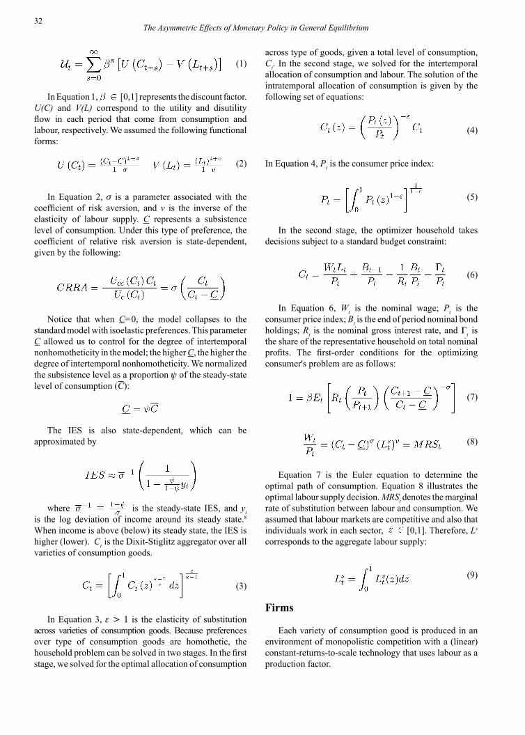
In Equation 1, [0,1] represents the discount factor. U(C) and V(L) correspond to the utility and disutility flow in each period that come from consumption and labour, respectively. We assumed the following functional forms:
(2)
In Equation 2, s is a parameter associated with the coefficient of risk aversion, and v is the inverse of the elasticity of labour supply. C represents a subsistence level of consumption. Under this type of preference, the coefficient of relative risk aversion is state-dependent, given by the following:
Notice that when C=0, the model collapses to the standard model with isoelastic preferences. This parameter C allowed us to control for the degree of intertemporal nonhomotheticity in the model; the higher C, the higher the degree of intertemporal nonhomotheticity. We normalized the subsistence level as a proportion y of the steady-state level of consumption (C):
The IES is also state-dependent, which can be approximated by
where is the steady-state IES, and yt is the log deviation of income around its steady state.8 When income is above (below) its steady state, the IES is higher (lower). Ct is the Dixit-Stiglitz aggregator over all varieties of consumption goods.
(3)
In Equation 3, e > 1 is the elasticity of substitution across varieties of consumption goods. Because preferences over type of consumption goods are homothetic, the household problem can be solved in two stages. In the first stage, we solved for the optimal allocation of consumption
across type of goods, given a total level of consumption, Ct. In the second stage, we solved for the intertemporal allocation of consumption and labour. The solution of the intratemporal allocation of consumption is given by the following set of equations:
(4)
In Equation 4, Pt is the consumer price index:
(5)
In the second stage, the optimizer household takes decisions subject to a standard budget constraint:
(6)
In Equation 6, Wt is the nominal wage; Pt is the consumer price index; Bt is the end of period nominal bond holdings; Rt is the nominal gross interest rate, and Gt is the share of the representative household on total nominal profits. The first-order conditions for the optimizing consumer's problem are as follows:
(7)
(8)
Equation 7 is the Euler equation to determine the optimal path of consumption. Equation 8 illustrates the optimal labour supply decision. MRSt denotes the marginal rate of substitution between labour and consumption. We assumed that labour markets are competitive and also that individuals work in each sector, [0,1]. Therefore, Ls
corresponds to the aggregate labour supply:
(9)
Firms
Each variety of consumption good is produced in an environment of monopolistic competition with a (linear) constant-returns-to-scale technology that uses labour as a production factor.
The Asymmetric Effects of Monetary Policy in General Equilibrium
33
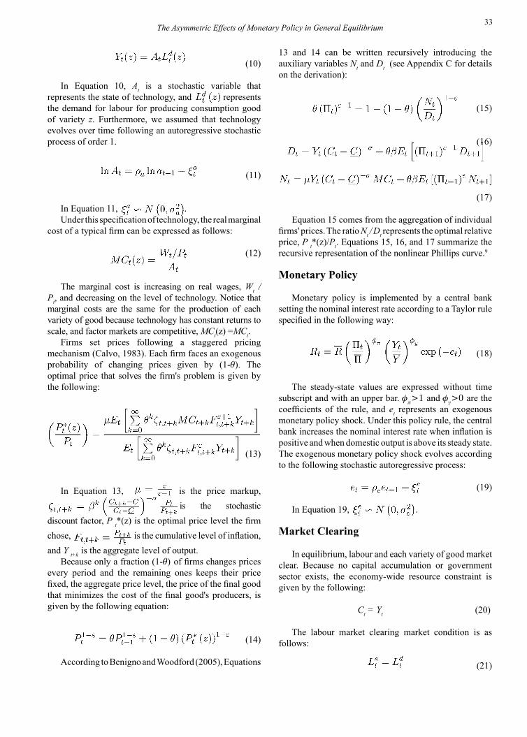
(10)
In Equation 10, At is a stochastic variable that represents the state of technology, and represents the demand for labour for producing consumption good of variety z. Furthermore, we assumed that technology evolves over time following an autoregressive stochastic process of order 1.
(11)
In Equation 11, .Under this specification of technology, the real marginal
cost of a typical firm can be expressed as follows:
(12)
The marginal cost is increasing on real wages, Wt /Pt, and decreasing on the level of technology. Notice that marginal costs are the same for the production of each variety of good because technology has constant returns to scale, and factor markets are competitive, MCt(z) =MCt.
Firms set prices following a staggered pricing mechanism (Calvo, 1983). Each firm faces an exogenous probability of changing prices given by (1-q). The optimal price that solves the firm's problem is given by the following:
(13)
In Equation 13, is the price markup, is the stochastic
discount factor, P t*(z) is the optimal price level the firm chose, is the cumulative level of inflation, and Y t+k
is the aggregate level of output.Because only a fraction (1-q) of firms changes prices
every period and the remaining ones keeps their price fixed, the aggregate price level, the price of the final good that minimizes the cost of the final good's producers, is given by the following equation:
(14)
According to Benigno and Woodford (2005), Equations
13 and 14 can be written recursively introducing the auxiliary variables Nt and Dt (see Appendix C for details on the derivation):
(15)
(16)
(17)
Equation 15 comes from the aggregation of individual firms' prices. The ratio Nt / Dt represents the optimal relative price, P t*(z)/Pt. Equations 15, 16, and 17 summarize the recursive representation of the nonlinear Phillips curve.9
Monetary Policy
Monetary policy is implemented by a central bank setting the nominal interest rate according to a Taylor rule specified in the following way:
(18)
The steady-state values are expressed without time subscript and with an upper bar. f
p>1 and f
g>0 are the
coefficients of the rule, and et represents an exogenous monetary policy shock. Under this policy rule, the central bank increases the nominal interest rate when inflation is positive and when domestic output is above its steady state. The exogenous monetary policy shock evolves according to the following stochastic autoregressive process:
(19)
In Equation 19, .
Market Clearing
In equilibrium, labour and each variety of good market clear. Because no capital accumulation or government sector exists, the economy-wide resource constraint is given by the following:
Ct = Yt (20)
The labour market clearing market condition is as follows:
(21)
The Asymmetric Effects of Monetary Policy in General Equilibrium
34
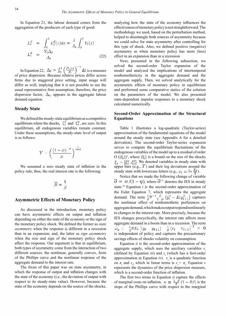
In Equation 21, the labour demand comes from the aggregation of the producers of each type of good:
(22)
In Equation 22, dz is a measure
of price dispersion. Because relative prices differ across firms due to staggered price setting, input usage will differ as well, implying that it is not possible to use the usual representative firm assumption; therefore, the price dispersion factor, , appears in the aggregate labour demand equation.
Steady State
We defined the steady-state equilibrium as a competitive equilibrium where the shocks, and , are zero. In this equilibrium, all endogenous variables remain constant. Under these assumptions, the steady-state level of output is as follows:
We assumed a zero steady state of inflation in the policy rule; thus, the real interest rate is the following:
Asymmetric Effects of Monetary Policy
As discussed in the introduction, monetary policy can have asymmetric effects on output and inflation depending on either the state of the economy or the sign of the monetary policy shock. We defined the former as state asymmetry when the response is different in a recession than in an expansion; and, the latter as sign asymmetry when the size and sign of the monetary policy shock affect the response. Our argument is that in equilibrium, both types of asymmetry come from the interaction of two different sources: the nonlinear, generally convex, form of the Phillips curve and the nonlinear response of the aggregate demand to the interest rate.
The focus of this paper was on state asymmetry, in which the response of output and inflation changes with the state of the economy (i.e., the deviation of output with respect to its steady-state value). However, because the state of the economy depends on the source of the shocks,
analyzing how the state of the economy influences the effectiveness of monetary policy is not straightforward. The methodology we used, based on the perturbation method, helped to disentangle both sources of asymmetry because we could solve for state asymmetry after controlling for this type of shock. Also, we defined positive (negative) asymmetry as when monetary policy has more (less) effect in an expansion than in a recession.
Next, presented in the following subsection, we solved the second-order Taylor expansion of the model and analyzed the implications of intertemporal nonhomotheticity in the aggregate demand and the aggregate supply. Then, we solved analytically for the asymmetric effects of monetary policy in equilibrium and performed some comparative statics of the solution on the parameters of the model. We also presented state-dependent impulse responses to a monetary shock calculated numerically.
Second-Order Approximation of the Structural Equations
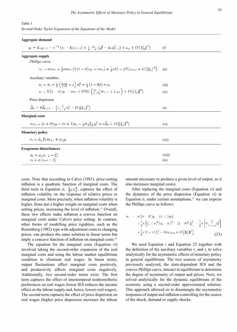
Table 1 illustrates a log-quadratic (Taylor-series) approximation of the fundamental equations of the model around the steady state (see Appendix A for a detailed derivation). The second-order Taylor-series expansion serves to compute the equilibrium fluctuations of the endogenous variables of the model up to a residual of order O (||xt||)
2, where ||xt|| is a bound on the size of the shocks . We denoted variables in steady state with
upper bars (e.g., X ) and their log deviations around the steady state with lowercase letters (e.g., ).
Notice that we made the following change of variable s s /(1 - y), where s-1 denotes the IES in steady state.10 Equation i is the second-order approximation of the Euler Equation 7, which represents the aggregate demand. The term
captures
the nonlinear effect of nonhomothetic preferences on aggregate demand, which makes output respond nonlinearly to changes in the interest rate. More precisely, because the IES changes procyclically, the interest rate affects more aggregate demand in a boom than in a recession. The term
< 0 is independent of policy and captures the precautionary savings effects of shocks volatility on consumption.
Equation ii is the second-order approximation of the aggregate supply, which uses the auxiliary variables vt (defined by Equation iii) and zt (which has a first-order approximation in Equation iv). vt is a quadratic function on πt and zt, which in linear terms is vt = πt. Equation v represents the dynamics of the price dispersion measure, which is a second-order function of inflation.
The first two terms in Equation ii capture the effects of marginal costs on inflation. is the slope of the Phillips curve with respect to the marginal
The Asymmetric Effects of Monetary Policy in General Equilibrium
35
costs. Note that according to Calvo (1983), price-setting inflation is a quadratic function of marginal costs. The third term in Equation ii, , captures the effect of inflation volatility on the response of relative prices to marginal costs. More precisely, when inflation volatility is higher, firms put a higher weight on marginal costs when setting prices, increasing the level of inflation.11 Overall, these two effects make inflation a convex function on marginal costs under Calvo's price setting. In contrast, other forms of modelling price rigidities, such as the Rotemberg (1982) type with adjustment costs to changing prices, can produce the same solution in linear terms but imply a concave function of inflation on marginal costs.12
The equation for the marginal costs (Equation vi) involved taking the second-order expansion of the real marginal costs and using the labour market equilibrium condition to eliminate real wages. In linear terms, output fluctuations affect marginal costs positively, and productivity affects marginal costs negatively. Additionally, two second-order terms exist: The first term captures the effect of intertemporal nonhomothetic preferences on real wages (lower IES reduces the income effect on the labour supply and, hence, lowers real wages). The second term captures the effect of price dispersion on real wages (higher price dispersion increases the labour
amount necessary to produce a given level of output, so it also increases marginal costs).
After replacing the marginal costs (Equation vi) and the dynamics of the price dispersion (Equation vi) in Equation ii, under certain assumptions,13 we can express the Phillips curve as follows:
(23)
We used Equation i and Equation 23 together with the definition of the auxiliary variables vt and zt to solve analytically for the asymmetric effects of monetary policy in general equilibrium. The two sources of asymmetry previously analyzed, the state-dependent IES and the convex Phillips curve, interact in equilibrium to determine the degree of asymmetry of output and prices. Next, we solved analytically for the dynamic equilibrium of the economy using a second-order approximated solution. This approach allowed us to disentangle the asymmetric responses of output and inflation controlling for the source of the shock, demand or supply shocks.
The Asymmetric Effects of Monetary Policy in General Equilibrium
Table 1Second-Order Taylor Expansion of the Equations of the Model
Aggregate demand
Aggregate supply Phillips curve Auxiliary variables Price dispersion
Marginal costs
Monetary policy
Exogenous disturbances
(i)
(ii)
(iii)
(iv)
(v)
(vi)
(vii)
(viii)(ix)
36
Solving Asymmetric Response Analytically
We used the perturbation method, developed by Judd (1998), Collard and Juillard (2001) and Schmitt-Grohé and Uribe (2004), to find a second-order approximation of the solution of the model. This method consisted in obtaining the coefficients of a Taylor expansion of the solution of the model near the steady state using a system of equations from the differentiation of the equilibrium conditions of the model (see Appendix C for a discussion of the implementation of this method). We approximated the policy functions for output and inflation as second-order polynomials on the state variables, s = [a,e], the productivity and monetary policy shocks, respectively. Furthermore, the former represents supply shocks, and the latter represents demand shocks:
(24)
In Equation 24, y and π are output and inflation in log deviations from the steady state. We initially assumed a log-linear policy rule of the following form:
The coefficients of the first-order terms {ba , be , da , de} are equal to those of the log-linearized solution of the model. The second-order solution only adds additional terms to the log-linearized solution, {bae , baa , bee , dae , daa , dee}, preserving the existing terms. Furthermore, b and d are constants that depend on the variance of the shocks, as shown in Schmitt-Grohé and Uribe (2004).
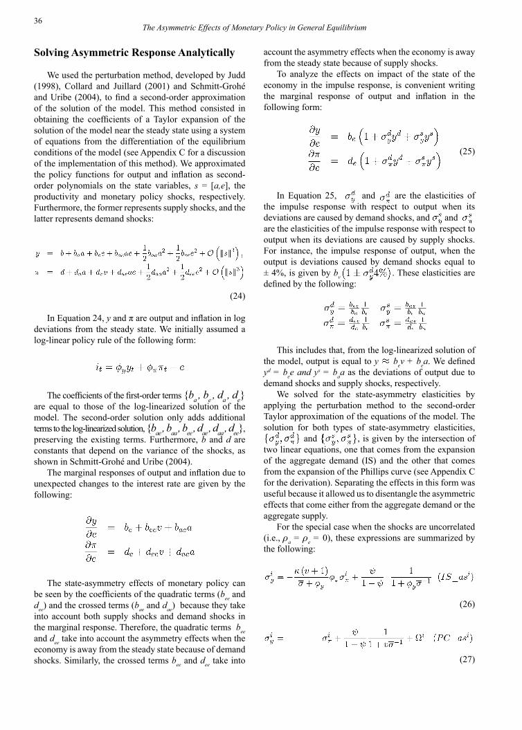
The marginal responses of output and inflation due to unexpected changes to the interest rate are given by the following:
The state-asymmetry effects of monetary policy can be seen by the coefficients of the quadratic terms (bee and dee) and the crossed terms (bae and dae) because they take into account both supply shocks and demand shocks in the marginal response. Therefore, the quadratic terms bee and dee take into account the asymmetry effects when the economy is away from the steady state because of demand shocks. Similarly, the crossed terms bee and dee take into
account the asymmetry effects when the economy is away from the steady state because of supply shocks.
To analyze the effects on impact of the state of the economy in the impulse response, is convenient writing the marginal response of output and inflation in the following form:
(25)
In Equation 25, and are the elasticities of the impulse response with respect to output when its deviations are caused by demand shocks, and and are the elasticities of the impulse response with respect to output when its deviations are caused by supply shocks. For instance, the impulse response of output, when the output is deviations caused by demand shocks equal to ± 4%, is given by bv . These elasticities are defined by the following:
This includes that, from the log-linearized solution of the model, output is equal to y bev + bea. We defined yd = bee and ys = baa as the deviations of output due to demand shocks and supply shocks, respectively.
We solved for the state-asymmetry elasticities by applying the perturbation method to the second-order Taylor approximation of the equations of the model. The solution for both types of state-asymmetry elasticities,
and , is given by the intersection of two linear equations, one that comes from the expansion of the aggregate demand (IS) and the other that comes from the expansion of the Phillips curve (see Appendix C for the derivation). Separating the effects in this form was useful because it allowed us to disentangle the asymmetric effects that come either from the aggregate demand or the aggregate supply.
For the special case when the shocks are uncorrelated (i.e., ra = re = 0), these expressions are summarized by the following:
(26)
(27)
The Asymmetric Effects of Monetary Policy in General Equilibrium
37
The index i = {d,s} indicates whether the output deviations occur through demand shocks (i = d) or supply shocks (i = s). Wd and Ws are defined in Appendix C and capture the nonlinearity of the Phillips curve. These schedules are named IS_asi and PC_asi because they come from the second-order expansion of the IS and the Phillips curve, respectively. The elasticities are found in equilibrium by the intersection of both equations.
The IS_asi schedule has a negative slope equal to , and the PC_asi schedule has a positive slope
equal to 1. Moreover, when y = 0, the intercept is zero for the IS_asi schedule and equal to Wi for the PC_asi, which can be either positive or negative. The state-asymmetry elasticities solution is given by the intersection of the two curves. In the next subsection, we analyze the equilibrium in two cases, for y = 0 and y > 0, and we perform some comparative statics with respect to some parameters.
Comparative Statics
The model was parameterized using values that are standard in the literature. We set a quarterly discount factor, b, equal to 0.99, which implies an annualized rate of interest of 4%. For the coefficient of risk-aversion parameter, s, we chose a value of 1 and calibrated the inverse of the elasticity of labour supply, v, to be equal to 1. We chose a degree of monopolistic competition, e, equal to 7.88, which implies a firm markup of 15% over the marginal cost. The probability of not adjusting prices, q, was set to 0.66, which implies that firms typically change prices every three quarters. We set the parameters of the Taylor rule f
p and fy to 1.5 and 0.5, respectively.
We assumed the same distribution for both productivity and monetary policy shocks, with a standard deviation of 0.1 and ra = re = 0.6 for the impulse response. Finally, the subsistence-consumption level was set to 0.8 of the steady-state level of output, similar to the values used in the habit-formation models.
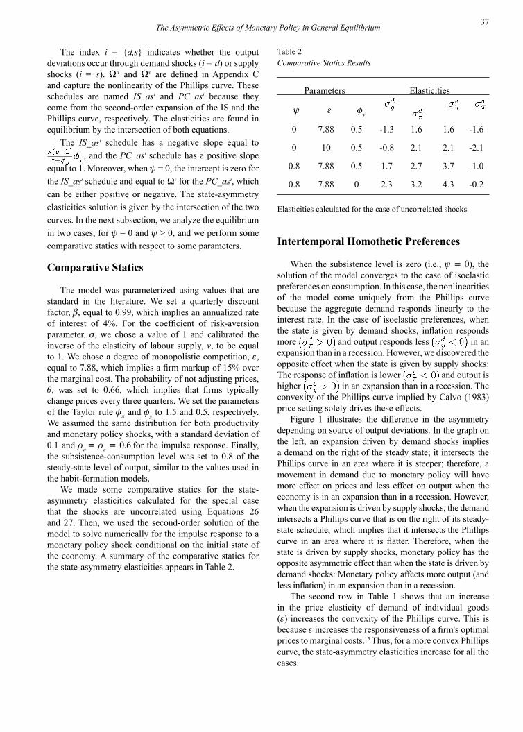
We made some comparative statics for the state-asymmetry elasticities calculated for the special case that the shocks are uncorrelated using Equations 26 and 27. Then, we used the second-order solution of the model to solve numerically for the impulse response to a monetary policy shock conditional on the initial state of the economy. A summary of the comparative statics for the state-asymmetry elasticities appears in Table 2.
Table 2Comparative Statics Results
Parameters Elasticities
y e fy
0 7.88 0.5 -1.3 1.6 1.6 -1.6
0 10 0.5 -0.8 2.1 2.1 -2.1
0.8 7.88 0.5 1.7 2.7 3.7 -1.0
0.8 7.88 0 2.3 3.2 4.3 -0.2
Elasticities calculated for the case of uncorrelated shocks
Intertemporal Homothetic Preferences
When the subsistence level is zero (i.e., y = 0), the solution of the model converges to the case of isoelastic preferences on consumption. In this case, the nonlinearities of the model come uniquely from the Phillips curve because the aggregate demand responds linearly to the interest rate. In the case of isoelastic preferences, when the state is given by demand shocks, inflation responds more and output responds less in an expansion than in a recession. However, we discovered the opposite effect when the state is given by supply shocks: The response of inflation is lower and output is higher in an expansion than in a recession. The convexity of the Phillips curve implied by Calvo (1983) price setting solely drives these effects.
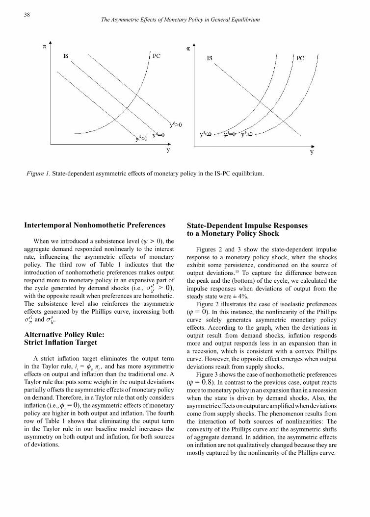
Figure 1 illustrates the difference in the asymmetry depending on source of output deviations. In the graph on the left, an expansion driven by demand shocks implies a demand on the right of the steady state; it intersects the Phillips curve in an area where it is steeper; therefore, a movement in demand due to monetary policy will have more effect on prices and less effect on output when the economy is in an expansion than in a recession. However, when the expansion is driven by supply shocks, the demand intersects a Phillips curve that is on the right of its steady-state schedule, which implies that it intersects the Phillips curve in an area where it is flatter. Therefore, when the state is driven by supply shocks, monetary policy has the opposite asymmetric effect than when the state is driven by demand shocks: Monetary policy affects more output (and less inflation) in an expansion than in a recession.
The second row in Table 1 shows that an increase in the price elasticity of demand of individual goods (e) increases the convexity of the Phillips curve. This is because e increases the responsiveness of a firm's optimal prices to marginal costs.15 Thus, for a more convex Phillips curve, the state-asymmetry elasticities increase for all the cases.
The Asymmetric Effects of Monetary Policy in General Equilibrium
38
Intertemporal Nonhomothetic Preferences
When we introduced a subsistence level (y > 0), the aggregate demand responded nonlinearly to the interest rate, influencing the asymmetric effects of monetary policy. The third row of Table 1 indicates that the introduction of nonhomothetic preferences makes output respond more to monetary policy in an expansive part of the cycle generated by demand shocks (i.e., > 0), with the opposite result when preferences are homothetic. The subsistence level also reinforces the asymmetric effects generated by the Phillips curve, increasing both
and .
Alternative Policy Rule:Strict Inflation Target
A strict inflation target eliminates the output term in the Taylor rule, it = fπ πt , and has more asymmetric effects on output and inflation than the traditional one. A Taylor rule that puts some weight in the output deviations partially offsets the asymmetric effects of monetary policy on demand. Therefore, in a Taylor rule that only considers inflation (i.e., fy = 0), the asymmetric effects of monetary policy are higher in both output and inflation. The fourth row of Table 1 shows that eliminating the output term in the Taylor rule in our baseline model increases the asymmetry on both output and inflation, for both sources of deviations.
State-Dependent Impulse Responsesto a Monetary Policy Shock
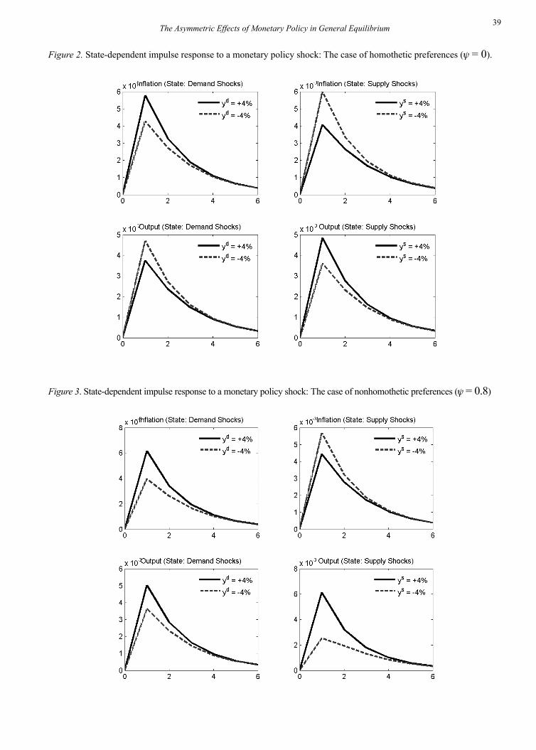
Figures 2 and 3 show the state-dependent impulse response to a monetary policy shock, when the shocks exhibit some persistence, conditioned on the source of output deviations.15 To capture the difference between the peak and the (bottom) of the cycle, we calculated the impulse responses when deviations of output from the steady state were ± 4%.
Figure 2 illustrates the case of isoelastic preferences (y = 0). In this instance, the nonlinearity of the Phillips curve solely generates asymmetric monetary policy effects. According to the graph, when the deviations in output result from demand shocks, inflation responds more and output responds less in an expansion than in a recession, which is consistent with a convex Phillips curve. However, the opposite effect emerges when output deviations result from supply shocks.
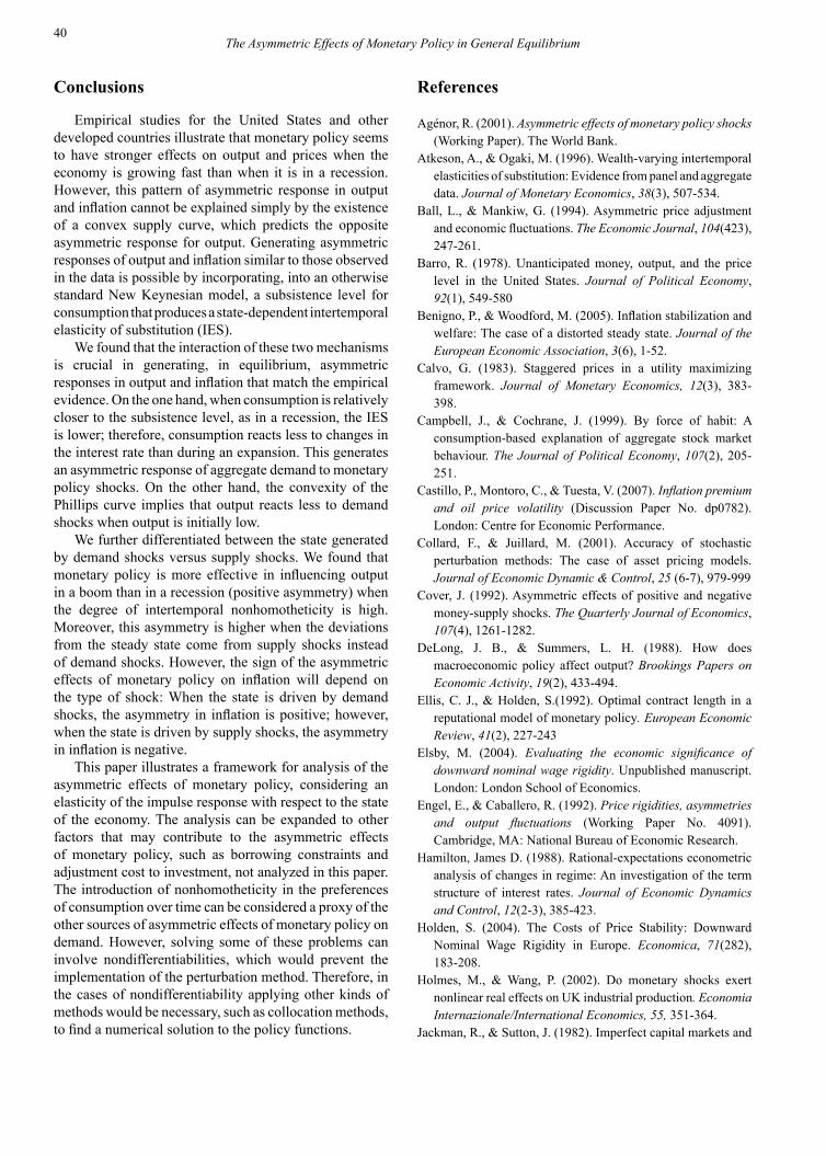
Figure 3 shows the case of nonhomothetic preferences (y = 0.8). In contrast to the previous case, output reacts more to monetary policy in an expansion than in a recession when the state is driven by demand shocks. Also, the asymmetric effects on output are amplified when deviations come from supply shocks. The phenomenon results from the interaction of both sources of nonlinearities: The convexity of the Phillips curve and the asymmetric shifts of aggregate demand. In addition, the asymmetric effects on inflation are not qualitatively changed because they are mostly captured by the nonlinearity of the Phillips curve.
The Asymmetric Effects of Monetary Policy in General Equilibrium
Figure 1. State-dependent asymmetric effects of monetary policy in the IS-PC equilibrium.
39The Asymmetric Effects of Monetary Policy in General Equilibrium
Figure 2. State-dependent impulse response to a monetary policy shock: The case of homothetic preferences (y = 0).
Figure 3. State-dependent impulse response to a monetary policy shock: The case of nonhomothetic preferences (y = 0.8)
40
Conclusions
Empirical studies for the United States and other developed countries illustrate that monetary policy seems to have stronger effects on output and prices when the economy is growing fast than when it is in a recession. However, this pattern of asymmetric response in output and inflation cannot be explained simply by the existence of a convex supply curve, which predicts the opposite asymmetric response for output. Generating asymmetric responses of output and inflation similar to those observed in the data is possible by incorporating, into an otherwise standard New Keynesian model, a subsistence level for consumption that produces a state-dependent intertemporal elasticity of substitution (IES).
We found that the interaction of these two mechanisms is crucial in generating, in equilibrium, asymmetric responses in output and inflation that match the empirical evidence. On the one hand, when consumption is relatively closer to the subsistence level, as in a recession, the IES is lower; therefore, consumption reacts less to changes in the interest rate than during an expansion. This generates an asymmetric response of aggregate demand to monetary policy shocks. On the other hand, the convexity of the Phillips curve implies that output reacts less to demand shocks when output is initially low.
We further differentiated between the state generated by demand shocks versus supply shocks. We found that monetary policy is more effective in influencing output in a boom than in a recession (positive asymmetry) when the degree of intertemporal nonhomotheticity is high. Moreover, this asymmetry is higher when the deviations from the steady state come from supply shocks instead of demand shocks. However, the sign of the asymmetric effects of monetary policy on inflation will depend on the type of shock: When the state is driven by demand shocks, the asymmetry in inflation is positive; however, when the state is driven by supply shocks, the asymmetry in inflation is negative.
This paper illustrates a framework for analysis of the asymmetric effects of monetary policy, considering an elasticity of the impulse response with respect to the state of the economy. The analysis can be expanded to other factors that may contribute to the asymmetric effects of monetary policy, such as borrowing constraints and adjustment cost to investment, not analyzed in this paper. The introduction of nonhomotheticity in the preferences of consumption over time can be considered a proxy of the other sources of asymmetric effects of monetary policy on demand. However, solving some of these problems can involve nondifferentiabilities, which would prevent the implementation of the perturbation method. Therefore, in the cases of nondifferentiability applying other kinds of methods would be necessary, such as collocation methods, to find a numerical solution to the policy functions.
References
Agénor, R. (2001). Asymmetric effects of monetary policy shocks (Working Paper). The World Bank.
Atkeson, A., & Ogaki, M. (1996). Wealth-varying intertemporal elasticities of substitution: Evidence from panel and aggregate data. Journal of Monetary Economics, 38(3), 507-534.
Ball, L., & Mankiw, G. (1994). Asymmetric price adjustment and economic fluctuations. The Economic Journal, 104(423), 247-261.
Barro, R. (1978). Unanticipated money, output, and the price level in the United States. Journal of Political Economy, 92(1), 549-580
Benigno, P., & Woodford, M. (2005). Inflation stabilization and welfare: The case of a distorted steady state. Journal of the European Economic Association, 3(6), 1-52.
Calvo, G. (1983). Staggered prices in a utility maximizing framework. Journal of Monetary Economics, 12(3), 383-398.
Campbell, J., & Cochrane, J. (1999). By force of habit: A consumption-based explanation of aggregate stock market behaviour. The Journal of Political Economy, 107(2), 205-251.
Castillo, P., Montoro, C., & Tuesta, V. (2007). Inflation premium and oil price volatility (Discussion Paper No. dp0782). London: Centre for Economic Performance.
Collard, F., & Juillard, M. (2001). Accuracy of stochastic perturbation methods: The case of asset pricing models. Journal of Economic Dynamic & Control, 25 (6-7), 979-999
Cover, J. (1992). Asymmetric effects of positive and negative money-supply shocks. The Quarterly Journal of Economics, 107(4), 1261-1282.
DeLong, J. B., & Summers, L. H. (1988). How does macroeconomic policy affect output? Brookings Papers on Economic Activity, 19(2), 433-494.
Ellis, C. J., & Holden, S.(1992). Optimal contract length in a reputational model of monetary policy. European Economic Review, 41(2), 227-243
Elsby, M. (2004). Evaluating the economic significance of downward nominal wage rigidity. Unpublished manuscript. London: London School of Economics.
Engel, E., & Caballero, R. (1992). Price rigidities, asymmetries and output fluctuations (Working Paper No. 4091). Cambridge, MA: National Bureau of Economic Research.
Hamilton, James D. (1988). Rational-expectations econometric analysis of changes in regime: An investigation of the term structure of interest rates. Journal of Economic Dynamics and Control, 12(2-3), 385-423.
Holden, S. (2004). The Costs of Price Stability: Downward Nominal Wage Rigidity in Europe. Economica, 71(282), 183-208.
Holmes, M., & Wang, P. (2002). Do monetary shocks exert nonlinear real effects on UK industrial production. Economia Internazionale/International Economics, 55, 351-364.
Jackman, R., & Sutton, J. (1982). Imperfect capital markets and
The Asymmetric Effects of Monetary Policy in General Equilibrium
41
the monetarist black box: Liquidity constraints, inflation and the asymmetric effects of interest rate policy. The Economic Journal, 92(365), 108-128.
Jaffee, D., & Stiglitz, J. (1990). Credit rationing. In B. Friedman, & F. Hahn (Eds.), The handbook of monetary economics. (Vol II. 837-888). Amsterdam: Elservier
Judd, K. (1998). Numerical Methods in Economics. Cambridge, MA: MIT Press
Karras, G., & Stokes, H. (1999). Why are the effects of money-supply shocks asymmetric? Evidence from prices, consumption and investment. Journal of Macroeconomics, 21(4), 713-727, 227-235.
Kim, J., & Kim, S. (2003). Welfare effects of tax policy in open economies: stabilization and cooperation. Finance and Economics Discussion Series 2003-51, Washington, DC: Board of Governors of the Federal Reserve System U.S.
Morgan, D. (1993). Asymmetric effects of monetary policy. Economic Review, Q II, 21-33. Kansas City, KS: Federal Reserve Bank of Kansas City.
Ravn, M., Schmitt-Grohé, S., & Uribe, M. (2006). Deep habits. Review of Economic Studies, 73(1), 195-218.
Ravn, M., & Sola, M. (1996). A reconsideration of the empirical evidence on the asymmetric effects of money-supply shocks: Positive vs. negative or big vs. small? Unpublished manuscript, University of Aarhus, Denmark.
Rotemberg, J. (1982). Sticky Prices in the United States, Journal of Political Economy, 90(6), 1187-1211.
Schmitt-Grohe, S., & Uribe, M. (2004). Solving dynamic general equilibrium models using a second-order approximation to the policy function. Journal of Economic Dynamics and Control, 28(4), 755-775.
Terasvirta, T., & Anderson, H. M. (1992). Characterizing nonlinearities in business cycles using smooth transition autoregressive models. Journal of Applied Econometrics, 7(S), S119-S136.
Thoma, M. (1994). Subsample instability and asymmetries in money-income causality. Journal of Econometrics, 64(1-2), 279-306.
Weise, C. (1999). The asymmetric effects of monetary policy: A nonlinear vector autoregression approach. Journal of Money, Credit and Banking, 31(1), 85-108.
Woodford, M. (2003). Interest and prices: Foundations of a theory of monetary policy. Princeton, NJ: Princeton University Press.
Footnotes
1 For example, see Jackman and Sutton (1982) and Ball and Mankiw (1994).
2 The definition of a general nonhomothetic utility function is a set of preferences that exhibits nonlinear Engel’s curves (i.e., the expenditure on good i increases nonlinearly with income). Nonhomotheticity is intertemporal when real income affects the profile of consumption across time and intratemporal
when real income affects consumption allocation across different goods over time.
3 The effect of intertemporal nonhomotheticity is in some sense similar to the effects of borrowing constraints on consumption because, with borrowing constraints, the level of income also affects the optimal path of consumption.
4 See Atkeson and Ogaki (1996).5 For models of wage rigidity based on optimal contract and
fairness considerations, see Ellis and Holden (1997) and Holden (2004). For a model of wage stickiness based on loss aversion, see Elsby (2004).
6 For models of credit rationing, see Jaffee and Stiglitz (1990).
7 This assumption is different from Woodford (2003), who assumed that each good uses a differentiated skill labour to generate strategic complementarity in pricing decisions.
8 Here we assumed a closed economy without capital or government expenditures.
9 Writing the optimal price setting in a recursive way is necessary to implement the perturbation method numerically or algebraically.
10 In all the following analysis, we replaced s-1=s-1(1-y), which is the IES in steady state with subsistence, and changed s-1 endogenously as y changed to keep s-1 constant. This allowed us to compare the effects of y on asymmetry without considering the effects caused by the change on the steady-state IES.
11 Also, as shown in Castillo, Montoro, and Tuesta (2007), the third term in Equation ii is important in generating a risk premium on inflation.
12 This is because in the Rotemberg (1982) setup, the adjustment costs are quadratic on price deviations. Higher price deviations from the steady-state level are relatively more costly to the firms than small deviations, making firms respond relatively less when deviations on marginal costs are higher.
13 More precisely, when the initial price dispersion is small (i.e., up to second order). This assumption makes the
analysis analytically tractable, without changing the results qualitatively.
14 See Castillo et al. (2007) for a more detailed discussion of the effects of e on the convexity of the Phillips curve.
15 The state-dependent impulse responses are calculated numerically from the second-order solution of the model, conditional to an initial value of output deviations equal to yt-1 = ±4%, and considering the definitions for the deviations of output due to demand shocks (yd = bee) and supply shocks (ys = baa).
16 The assumption that the initial price dispersion is small makes the analysis analytically tractable, without changing the results qualitatively.
* Correspondence concerning this article should be addressed to Carlos Montoro, Jr. Miroquesada #441, Lima-Perú. Tel: (511)-613-2060. E-mail: [email protected].
The Asymmetric Effects of Monetary Policy in General Equilibrium
42The Asymmetric Effects of Monetary Policy in General Equilibrium
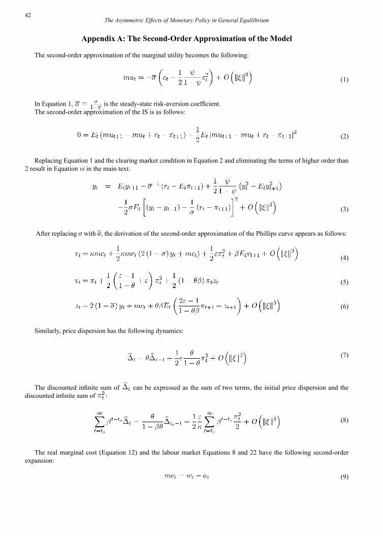
Appendix A: The Second-Order Approximation of the Model
The second-order approximation of the marginal utility becomes the following:
(1)
In Equation 1, is the steady-state risk-aversion coefficient. The second-order approximation of the IS is as follows:
(2)
Replacing Equation 1 and the clearing market condition in Equation 2 and eliminating the terms of higher order than 2 result in Equation vi in the main text:
(3)
After replacing s with s, the derivation of the second-order approximation of the Phillips curve appears as follows:
(4)
(5)
(6)
Similarly, price dispersion has the following dynamics:
(7)
The discounted infinite sum of can be expressed as the sum of two terms, the initial price dispersion and the discounted infinite sum of :
(8)
The real marginal cost (Equation 12) and the labour market Equations 8 and 22 have the following second-order expansion:
(9)
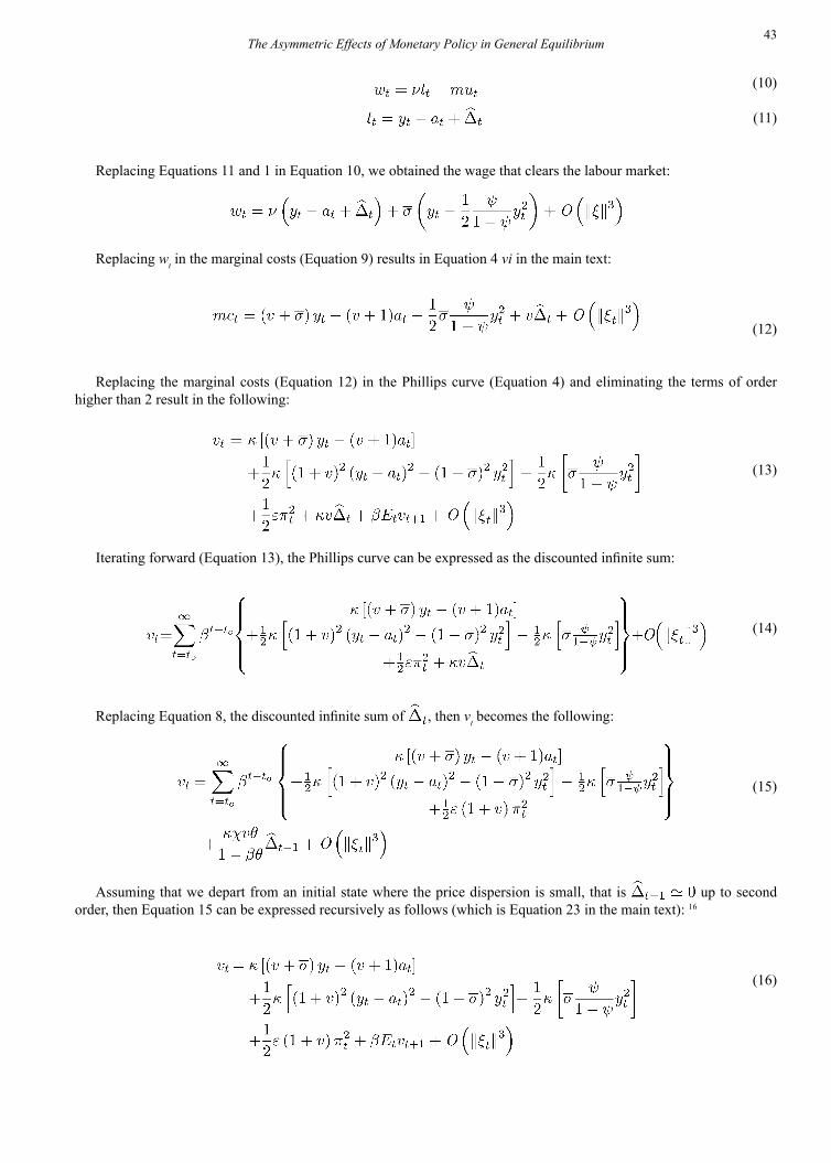
43The Asymmetric Effects of Monetary Policy in General Equilibrium
(10)
(11)
Replacing Equations 11 and 1 in Equation 10, we obtained the wage that clears the labour market:
Replacing wt in the marginal costs (Equation 9) results in Equation 4 vi in the main text:
(12)
Replacing the marginal costs (Equation 12) in the Phillips curve (Equation 4) and eliminating the terms of order higher than 2 result in the following:
(13)
Iterating forward (Equation 13), the Phillips curve can be expressed as the discounted infinite sum:
(14)
Replacing Equation 8, the discounted infinite sum of , then vt becomes the following:
(15)
Assuming that we depart from an initial state where the price dispersion is small, that is up to second order, then Equation 15 can be expressed recursively as follows (which is Equation 23 in the main text): 16
(16)
44The Asymmetric Effects of Monetary Policy in General Equilibrium
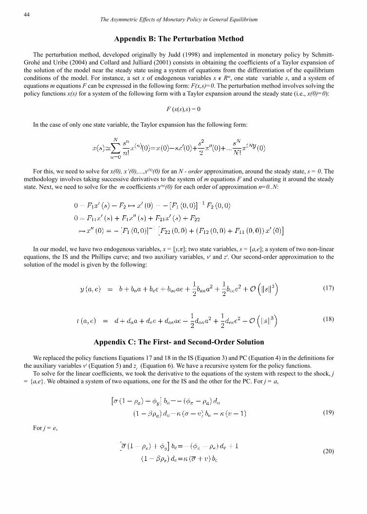
Appendix B: The Perturbation Method
The perturbation method, developed originally by Judd (1998) and implemented in monetary policy by Schmitt-Grohé and Uribe (2004) and Collard and Julliard (2001) consists in obtaining the coefficients of a Taylor expansion of the solution of the model near the steady state using a system of equations from the differentiation of the equilibrium conditions of the model. For instance, a set x of endogenous variables x e Rm, one state variable s, and a system of equations m equations F can be expressed in the following form: F(x,s)=0. The perturbation method involves solving the policy functions x(s) for a system of the following form with a Taylor expansion around the steady state (i.e., x(0)=0):
F (x(s),s) = 0
In the case of only one state variable, the Taylor expansion has the following form:
For this, we need to solve for x(0), x’(0),...,x(N)(0) for an N - order approximation, around the steady state, s = 0. The methodology involves taking successive derivatives to the system of m equations F and evaluating it around the steady state. Next, we need to solve for the m coefficients x(n)(0) for each order of approximation n=0..N:
In our model, we have two endogenous variables, x = [y,π]; two state variables, s = [a,e]; a system of two non-linear equations, the IS and the Phillips curve; and two auxiliary variables, vt and zt. Our second-order approximation to the solution of the model is given by the following:
(17)
(18)
Appendix C: The First- and Second-Order Solution
We replaced the policy functions Equations 17 and 18 in the IS (Equation 3) and PC (Equation 4) in the definitions for the auxiliary variables vt (Equation 5) and zt (Equation 6). We have a recursive system for the policy functions.
To solve for the linear coefficients, we took the derivative to the equations of the system with respect to the shock, j = {a,e}. We obtained a system of two equations, one for the IS and the other for the PC. For j = a,
(19)
For j = e,
(20)
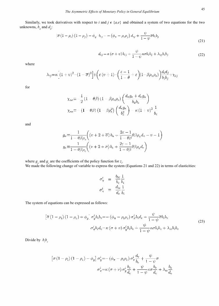
45
Similarly, we took derivatives with respect to i and j e {a,e} and obtained a system of two equations for the two unknowns, bij and dij:
(21)
(22)
where
for
and
where ga and ge are the coefficients of the policy function for zt.We made the following change of variable to express the system (Equations 21 and 22) in terms of elasticities:
The system of equations can be expressed as follows:
(23)
Divide by bibe
The Asymmetric Effects of Monetary Policy in General Equilibrium
46
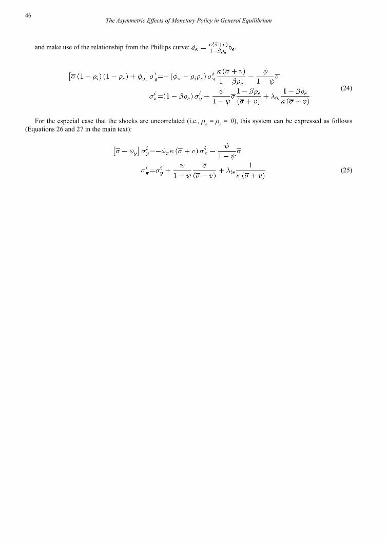
and make use of the relationship from the Phillips curve: .
(24)
For the especial case that the shocks are uncorrelated (i.e., ra = re = 0), this system can be expressed as follows (Equations 26 and 27 in the main text):
(25)
The Asymmetric Effects of Monetary Policy in General Equilibrium
Recommended