US Monetary Policy Rules: the Casefor Asymmetric Preferences

Paolo Surico¤Bocconi University

November 2002

Abstract

This paper investigates the empirical relevance of a new framework for monetary policy

analysis in which decision makers are allowed to weight di¤erently positive and negative

deviations of in‡ation and output from the target values. The speci…cation of the central

bank objective is general enough to nest the symmetric quadratic form as a special case,

thereby making the derived policy rule potentially nonlinear. This forms the basis of our

identi…cation strategy which is used to develop a formal hypothesis testing for the presence

of asymmetric preferences. Reduced-form estimates of postwar US policy rules indicate

that the preferences of the Fed have been highly asymmetric with respect to both in‡ation

and output gaps, with the latter being the dominant source of nonlinearity after 1983.

JEL Classi…cation: C52, E52.

Keywords: nonlinear optimal monetary policy rules, asymmetric loss function, linearized

central bank Euler equation

¤WORD COUNT (including references, tables and …gures): 7728. .I am indebted to Larry Christiano, Richard Dennis, Carlo Favero, Charles Goodhart, Anton Muscatelli, UlfSöderström and Guido Tabellini for stimulating discussions. I wish to thank seminar participants at the Eu-ropean Central Bank, the University of Copenhagen, and the 2002 Workshop on Macroeconomic Dynamics atthe Chatolic University of Milan, as well as Stefania Albanesi, Efrem Castelnuovo, Nicola Curci, Matteo Man-era, Chris Martin, Costas Milas, Tommaso Monacelli, Gaia Narciso, Giorgio Primiceri, Saverio Simonelli andPietro Tommasino for useful comments. Address for correspondence: Istituto di Economia Politica, UniversitàBocconi, Via Gobbi 5, 20136 Milan, Italy. E-mail: paolo.surico@uni-bocconi.it

1

1 Introduction

The last decade has been characterized by an increasing consensus in monetary policy analy-

sis. One of the most in‡uential paradigm has been the design of policy interventions as the

constrained optimum of a well-behaved control problem in which the central bank moves in-

terest rates to minimize some quadratic criterion. The latter de…nes the ultimate goals of

monetary policy and translates the behavior of the target variables into some measure for pol-

icy evaluations. When assigned with such a problem, the central bank faces the constraints

representing the structure of the economy. The quadratic characteristic of the objective and

the linear feature of the constraints give rise to a linear …rst order condition according to

which monetary authorities move policy rates as the optimal response to the developments in

the economy.

While the quadratic speci…cation implies that monetary authorities evenly weight positive

and negative deviations of in‡ation and output from the target values, such a modeling choice

has been questioned by several practitioners at the policy committees of various central banks

on the ground that it has little justi…cation beyond analytical tractability (see Blinder, 1997,

and Goodhart, 1999). The few notable exceptions include Rotemberg and Woodford (1999)

and Woodford (2002, Ch. 6) who show that the quadratic form can be obtained as a sec-

ond order approximation of the utility-based welfare function. More generally, a number of

quadratic objectives have been recently proposed in the literature as a way to evaluate alter-

native targeting schemes and the policy recommendations have been implicitly drawn upon

the assumption of symmetric central bank preferences.1

Several recent studies however explore some novel mechanism through which the costs

of the business cycle can be asymmetric. Galì, Gertler and Lopez-Salido (2002) construct a

theoretical measure of welfare gap for the US based on price and wage markups, and show

that the costs of output ‡uctuations have been historically large and asymmetric. Erosa and

Ventura (2002) introduce transaction costs and heterogeneity in portfolio holdings in a neo-

classical model of the business cycle and …nd that those frictions make the costs of in‡ation

variation asymmetric. The psychology of choice suggests that people tend to place a greater

weight on the prospect of losses than on the prospect of gains in decision making under

uncertainty (see Kahneman and Tversky, 1979). Then, mutatis mutandis, policy makers who

aggregate over individual welfare may be loss-averse with respect to both in‡ation and output.

Lastly, as argued by Blinder (1997) the di¤erent political pressures faced by the central bank

over the business cycle are likely to translate into asymmetric interest rate responses.1See for instance Rudebusch and Svensson (1999), Dennis (2002), Söderström (2001) and Walsh (2002).

2

Despite of its intuitive appeal, only few studies have attempted to identify asymmetric

central bank behaviors and the relevance of this alternative framework remains to be assessed.

Chadha and Schellekens (1999) study the implications of nonquadratic loss functions in the

face of additive and multiplicative uncertainty, and …nd that asymmetric preferences are not

su¢cient to deliver a gradualist path of interest rates. Gerlach (2000), Dolado, Maria-Dolores

and Naveira (2002), and Martin and Milas (2001) show some international evidence that

supports the notion of asymmetric reaction functions. Ruge-Murcia (2002), and Cukierman

and Muscatelli (2002) study analytically the implicit functional form of a nonlinear policy

rule and conclude that the qualitative features of some G7 economy reaction functions are

consistent with an asymmetric objective. Dolado, Maria-Dolores and Ruge-Murcia (2002)

estimate an interest rate rule which is drawn upon the existence of asymmetric preferences on

in‡ation only, and …nd that US monetary policy can be characterized by a nonlinear reaction

function after 1983, but not before 1979.

This paper contributes to the theoretical and empirical literature on optimal monetary

policy rules in di¤erent respects. First, assuming a fairly general speci…cation of both in‡a-

tion and output objectives, we derive a closed-form solution of the optimal monetary policy

within a New-Keynesian model of the business cycle. Since our objective function nests the

conventional quadratic form as a special case, the speci…cation of the policy rule is shown

to be nonlinear if and only if the central bank preferences are asymmetric. This condition

delivers a formal theoretical prediction which can be successfully tested for. Second, the ana-

lytical approach to the solution of the central bank optimal control problem allows to identify

the degree of nonlinearities and asymmetries with respect to both in‡ation and output gaps,

a result that to our knowledge of the existing literature comes as new. Third, a linearized

version of the model predicts that the monetary authorities respond not only to the level of

in‡ation and output gaps (as suggested by Taylor, 1993) but also to their squared values.

Fourth, reduced-form estimates of US monetary policy rules indicate that nonlinearity is a

robust feature of the data over both the pre- and post-Volcker periods. While this …nding

enriches the picture provided by Clarida, Galì and Gertler (2000), it suggests that the pref-

erences of the Fed have been highly asymmetric in both in‡ation and output gaps, with the

asymmetries on the latter becoming more pronounced than those on the former after 1983.

The road map of the paper is as follows. Section 2 presents the theoretical model and

derives the interest rate rule as the …rst order condition of the central bank optimal control

problem. The identi…cation method and the hypothesis testing strategy for the presence of

asymmetric preferences are described in Section 3. Reduced-form estimates on postwar US

data are reported and discussed in the following part while the last Section concludes.

3

2 Theoretical model: a New-Keynesian perspective

We assume that the central bank conducts monetary policy through a targeting rule according

to the terminology of Svensson (1999). Thus, all available information are used to bring at

each point in time the target variables in line with their targets by penalizing any future

deviation of the former from the latter. The policy rule is modeled as the outcome of an

intertemporal optimization problem in which decision makers minimize a given criterion under

the constraints provided by the structure of the economy. The optimizing device allows us to

reversely engineer the objectives of the monetary authorities, which are unobservable, from

the observed path of policy rates implying that evidence on the latter can be interpreted as

informative about the former. Since our identi…cation strategy relies on the estimation of a

model-based speci…cation for the reaction function, we challenge the assumption of symmetric

policy preferences in the context of a popular framework for monetary policy analysis. This is

a version of the celebrated New-Keynesian model of the business cycle derived in Yun (1996),

and Woodford (2002, Ch. 3 and 4), among others.

2.1 The structure of the economy

This subsection describes an aggregate version of the New-Keynesian forward-looking model

with sticky prices that has been recently summarized by Clarida, Galì and Gertler (1999).

The evolution of the state variables is compactly represented by the following two-equation

system:

¼t = µEt¼t+1 + kyt + "st (1)

yt = Etyt+1 ¡ ' (it ¡ Et¼t+1) + "dt (2)

Equation (1) captures in a log-linear fashion the staggered feature of a Calvo-type world

in which each …rm adjusts its price with a constant probability in any given period, and

independently from the time elapsed from the last adjustment. The discrete nature of price

setting creates an incentive to adjust prices by more the higher is the future in‡ation expected

at time t. The in‡ation level is ¼t whereas the output gap is denoted by yt and captures the

movements in marginal costs associated with variations in excess demand. Equation (2) is a

log-linearized version of a standard Euler equation for consumption combined with the relevant

market clearing condition. It basically brings the notion of consumption smoothing into an

aggregate demand formulation by making output gap a positive function of its expected future

value and a negative function of the real interest rate, it ¡ Et¼t+1. Lastly, "st and "dt are a

well-behaved cost shock and demand shock, respectively.

4

2.2 An asymmetric speci…cation of the loss function

An important aspect of monetary policy making in such a model is that policy actions are

taken before the realization of economic shocks and therefore before the state variables are

determined. Accordingly, the central bank objective is to choose a path for interest rates at

the beginning of period t conditional upon the information available at the end of the previous

period. This timing device is captured by the following intertemporal criterion:

Minfitg

Et¡11X

¿=0

±¿Lt+¿ (3)

where ± is the discount factor and L stands for the period loss function.

Our framework di¤ers from the conventional quadratic set up in that we employ a more

general speci…cation of the monetary authorities’ objectives. Indeed, the quadratic form may

approximate reasonably well a number of di¤erent functions and in the absence of a rigorous

theoretical foundation any speci…c nonquadratic proposal is destined to be unsatisfactory

against the wide range of plausible alternatives. Hence, rather than attempting to uncover

the correct functional form of policy makers’ preferences, we evaluate the symmetric quadratic

paradigm upon the empirical merits of the monetary policy rule that this speci…cation implies.

With this descriptive scope in mind, we write Lt as follows:

Lt =e[®(¼t¡¼¤)] ¡ ® (¼t ¡ ¼¤) ¡ 1

®2 + ¸

"e(°yt) ¡ °yt ¡ 1

°2

#+

¹2

(it ¡ i¤)2 (4)

The coe¢cients ¸ and ¹ represent the central bank’s aversion towards output ‡uctuations

around potential and interest rate level ‡uctuations around the target i¤. The policy prefer-

ence towards in‡ation stabilization is normalized to one and therefore ¸ and ¹ are expressed

in relative terms. The in‡ation target is ¼¤ whereas the parameters ® and ° capture any

asymmetry in the objective function of the monetary authorities.

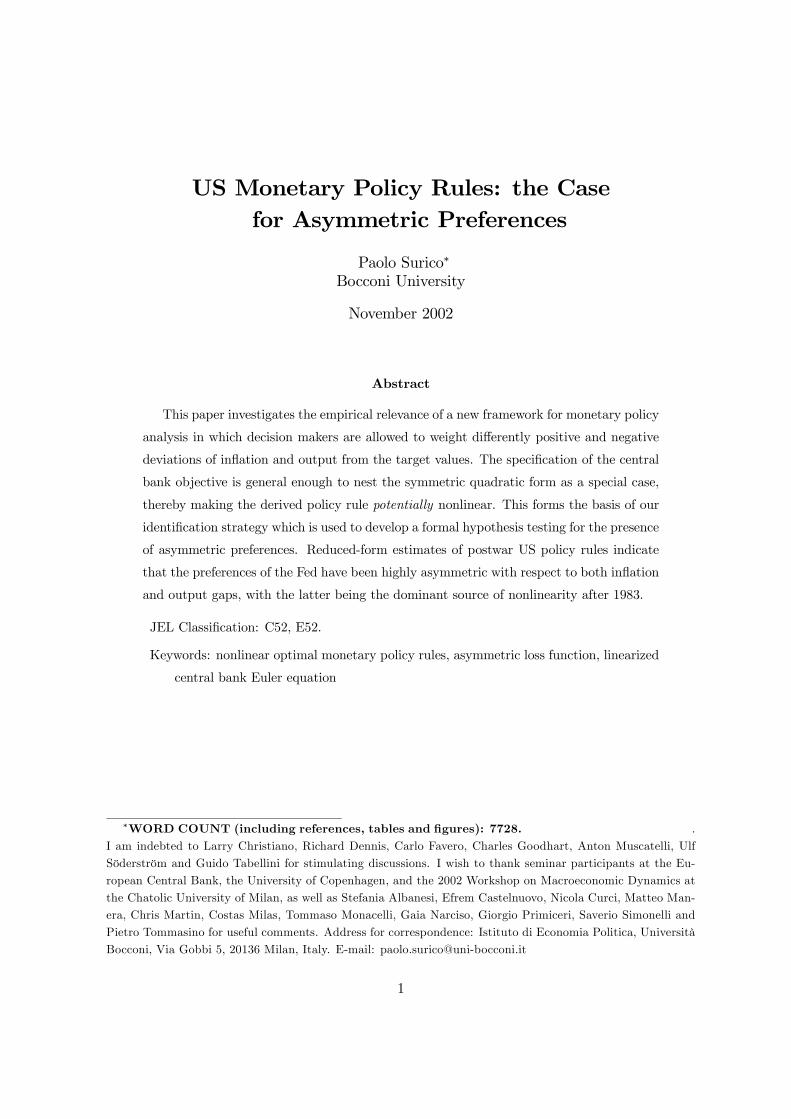
The linex speci…cation in (4), which has been originally proposed by Varian (1974) and

Zellner (1986) in the context of Bayesian econometric analysis and introduced by Nobay

and Peel (1998) in the optimal monetary policy literature, embodies a number of appealing

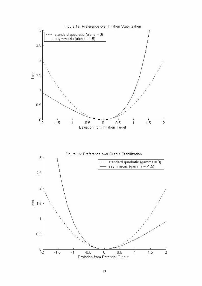
characteristics. First, it allows for departures from the quadratic objective in that policy

makers may treat di¤erently positive and negative deviations of the target variables from the

reference values. This pattern is shown in Figure 1 which plots the standard quadratic versus

the asymmetric function for both in‡ation (Panel a) and output gap (Panel b).

The key di¤erence between the two speci…cations is that deviations of the same size yield

di¤erent losses. Indeed, under the symmetric scenario policy makers are assumed to care

5

only about the magnitude of deviations whereas under asymmetric preferences they care also

about the sign. In particular, a positive value of ® in Panel (a) implies that, everything

equals, deviations of in‡ation (relative to target) from above are weighted more severely than

deviations from below. To see this notice that whenever ¼t¡¼¤ > 0 the exponential component

of the loss function dominates the linear component while the converse is true for ¼t¡¼¤ < 0.

The same reasoning holds for the coe¢cient ° in Panel (b), which captures any asymmetry in

the policy preferences for stabilizing the business cycle. However, if monetary authorities are

more concerned about undershooting potential output rather than overshooting it, the value

of ° would be negative implying that whenever y < 0 the loss rises exponentially whereas it

does linearly for y > 0.

Furthermore, the linex loss function speci…ed above is so general as to collapse to the

symmetric quadratic form for some parameter limiting case. Applying twice L’Hôpital’s rule

on (4), it is possible to show that whenever ® and ° tend to zero the central bank objective

function reduces to the symmetric parametrization Lt = 12

h(¼t ¡ ¼¤)2 + ¸y2t + ¹ (it ¡ i¤)2

i.

The latter can be obtained as a quadratic approximation of the utility-based welfare function

in a New-Keynesian model of the business cycle that involves a zero lower bound for nominal

interest rate (see Woodford, 2002, Ch. 6). Accordingly, the policy preferences would be

functions of some primitive parameters of the model implying that potential evidence of

asymmetries in the central bank objective could be tracked into evidence of asymmetries in

the representative agent’s utility. Indeed, as argued by Clarida, Galì and Gertler (1999), the

representative agent approach can be highly misleading as a guide to welfare analysis and it

is likely to be the case that some groups su¤er more in recessions or in high in‡ation periods

than others. This suggests that an asymmetric utility-based speci…cation of the loss function

may be a desirable representation of the social costs of cyclical ‡uctuations.

2.3 A nonlinear policy rule

We let monetary authorities choose policy rates in a discretionary fashion. Indeed, the case

for an optimal monetary policy without commitment seems to be closer to the actual practice

of many central banks which rarely tie their hands over the course of future policy actions.

Because no endogenous state variable enters the model, the intertemporal policy problem

reduces to a sequence of static optimization problems. This amounts to choosing in each

period the instrument rate such as to minimize:

Et¡1

Ãe[®(¼t¡¼¤)] ¡ ® (¼t ¡ ¼¤) ¡ 1

®2

!+ ¸Et¡1

"e(°yt) ¡ °yt ¡ 1

°2

#+

¹2

(it ¡ i¤)2 + Ft

6

subject to ¼t = kyt + ft and yt = ¡'it + gt where Ft ´ Et¡1P1¿=1 ±¿Lt+¿ , ft ´ µEt¼t+1 + "st

and gt ´ Etyt+1+'Et¼t+1+"dt are taken as given re‡ecting the fact that monetary authorities

cannot directly manipulate expectations. The …rst order condition reads

¡Et¡1

Ãe[®(¼t¡¼¤)] ¡ 1

®

!k' ¡ Et¡1

Ãe(°yt) ¡ 1

°

!¸' + ¹ (it ¡ i¤) = 0 (5)

which is a closed-form solution for the optimal policy rule. Equation (5) implicitly describes

a general reaction function according to which the central bank moves policy rates as the

optimal, potentially nonlinear, response to the developments in the economy.2 The important

result which underlies equation (5) is that it nests the conventional linear form as a special

case. Indeed, it can be shown by means of L’Hôpital’s rule that when both ® and ° tend to

zero the reaction function (5) collapses to an implicit interest rate rule of the type proposed

by Rudebusch (2002), and Clarida, Galì and Gertler (2000):

¡k'Et¡1 (¼t ¡ ¼¤) ¡ ¸'Et¡1 (yt) + ¹ (it ¡ i¤) = 0

This feature is attractive in that it delivers a joint restriction on policy makers’ preferences

which can be formally tested for. It follows that the hypothesis of symmetric loss function

can be challenged by assessing whether the relevant feedback coe¢cients are, either jointly or

marginally, signi…cantly di¤erent from zero. The policy parameters ® and ° are indeed crucial

for the analysis of optimal monetary policy not only because they introduce an asymmetric

motive in the central bank objective function but also because, more importantly, they make

those asymmetries mapping into a nonlinear policy rule. This suggests that were ® and °

identi…ed, the hypothesis that central bank preferences are symmetric around the target could

be tested simply by evaluating the functional form of the feedback rule as the latter would

correspond to test whether ® and ° are signi…cantly di¤erent from zero. Hence, evidence of

nonlinearity in the policy rule would be informative about which type of asymmetry, if any,

is relevant to policy makers.

3 Econometric analysis

The parameters ® and ° and the exponential function govern the asymmetric response of

policy rates to positive and negative deviations of the state variables from the target. Our

task consists in estimating the nonlinear reaction function (5) in order to evaluate whether2Notice that in contrast to other studies which impose an ad-hoc partial adjustment mechanism, our model-

based reaction function does not include any lagged interest rate terms. This comes from the fact that monetaryauthorities pursue the stabilization of policy rate levels rather than changes, a feature which hinges upon thespeci…cation of the utility function of the representative agent (see Woodford, 2002, Ch. 6).

7

those parameters are signi…cantly di¤erent from zero. This amounts to test linearity against

a nonlinear model, which is complicated by the fact that in small samples the estimation

criterion is insensitive to the so-called smoothness coe¢cients as there exists a large set of

®- and °-values yielding almost the same interest rate behavior (see Granger and Teräsvirta,

1993, Ch. 7). It follows that the asymmetric preferences would be inaccurately estimated,

thereby making the hypothesis testing for the presence of nonlinearities theoretically ‡awed.

Moreover, the speci…cation in (5) is nonlinear in the relevant parameters and therefore the

econometric method of estimation may pick up just one among the numerous local maxima

depending on the initial values of the coe¢cients.

A simple transformation of the model that confronts directly the issue involves the lin-

earization of the exponential terms in (5) by means of a …rst-order Taylor series expansion

around ® = ° = 0. The reduced-form policy rule now reads

¡k'Et¡1 (¼t ¡ ¼¤) ¡ ¸'Et¡1 (yt) ¡ ®k'2

Et¡1h(¼t ¡ ¼¤)2

i+

¡¸'°2

Et¡1¡y2t

¢+ ¹ (it ¡ i¤) + et = 0 (6)

with et being the remainder of the Taylor series approximation.

This condition relates the policy rates with the expected future levels and squared values

of the state variables conditioned upon the information available at time t ¡ 1. We solve

equation (6) for it and prior to estimation we replace expected in‡ation and output gaps with

actual values. Accordingly, we focus on the following policy rule:

it = const + c1¼t + c2yt + c3 (¼t)2 + c4 (yt)2 + vt (7)

which is linear in the coe¢cients

const ´ i¤ ¡ c1¼¤ ¡ c3 (¼¤)2

c1 ´ k'¹

¡ 2c3¼¤

c2 ´ ¸'¹

c3 ´ ®k'2¹

c4 ´ ¸'°2¹

and whose error term is de…ned as

vt ´ ¡(

c1 (¼t ¡ Et¡1¼t) + c2 (yt ¡ Et¡1yt)++c3

h¼2t ¡ Et¡1 (¼t)2

i+ c4

hy2t ¡ Et¡1 (yt)2

i)

+et¹

8

The term in curly brackets is a linear combination of forecast errors and therefore vt is or-

thogonal to any variable in the information set available at time t ¡ 1.

Equation (7) makes clear that by assuming an optimizing central bank behavior the reac-

tion function parameters can only be interpreted as convolutions of the coe¢cients representing

policy makers’ preferences and those describing the structure of the economy. While recover-

ing all structural parameters is beyond the scope of this paper, a single-equation estimation

of the derived policy rule is all we need to identify the asymmetric preferences. Indeed, the

feedback coe¢cients c3 and c4 embody the relevant information such that the joint restric-

tion ® = ° = 0 implies c1 6= 0, c2 6= 0 and c3 = c4 = 0. Hence, testing the hypothesis

H0 : ® = ° = 0 in (5) is equivalent to testing the hypothesis H 00 : c3 = c4 = 0 in (7).3 Un-

der the null of a linear reaction function, which fully corresponds to symmetric preferences,

the test statistics has an asymptotic Â2 distribution with as many degrees of freedom as the

number of restrictions. Such an hypothesis can be successfully evaluated through a standard

Wald test and since we are considering the auxiliary null H 00 : c3 = c4 = 0 rather than the

original hypothesis H0 : ® = ° = 0, the statistics is usually referred to as Wald-type.4

While our strategy allows to identify the asymmetric preference on output gap, °, from

the coe¢cients c4 and c2 only, it does not allow to recover the other key preference parameter,

®, unless some additional restriction are imposed to the policy rule. Nevertheless, were c3and c4 jointly signi…cant the hypothesis on symmetric preferences would be rejected. We will

return on the issue in the next section.

Lastly, it should be noticed that while the nonlinear quadratic terms in (7) stem from

asymmetric central bank preferences, we cannot exclude in principle that a nonlinear Phillips

curve be indeed responsible for any reduced-form evidence of nonlinearity. A simple way

to discriminate between nonquadratic objectives and nonlinear constraints is to perform the

REgression Speci…cation Error Test (RESET), which is designed to detect incorrect functional

forms, on the New-Keynesian Phillips curve. Accordingly, we estimate equation (1) on US

1960:1-2001:4 quarterly data using the Generalized Method of Moments (GMM) with a 12-

lag Newey-West variance covariance matrix. The set of instruments include four lags of GDP

chain-weighted in‡ation, Congressional Budget O¢ce output gap, long-short interest rate

spread, and consumer price in‡ation. When the squares and then the squares and the cubes

of the predictions ¼̂t are added to the original equation, the corresponding F-tests show that3 It is worthwhile to notice that the power of the test upon the auxiliary regression (7) crucially depends on

the signi…cance of c1 and c2 as it may be the case that H 00 cannot be rejected simply because c1 and c2 are notstatistically di¤erent from zero.

4As we are estimating a model which is linear in the parameters, the critique that the Wald test for nonlinearspeci…cations is not invariant to the parametrization of the model simply does not apply here.

9

the null hypothesis of non-misspeci…cation cannot be rejected. This suggests that the US

aggregate supply curve is well approximated by a linear relation, thereby making asymmetric

preferences the most empirically relevant source of nonlinearity over the sample. Empirical

support for a linear US Phillips curve can also be found in Dolado, Maria-Dolores and Ruge-

Murcia (2002), and Dolado, Maria-Dolores and Naveira (2002).

4 Empirical results

This section reports the estimates and the relevant tests of the policy reaction function (7).

The analysis is conducted on US quarterly data spanning the period 1960:1-2001:4. The

data set has been obtained from the web site of the Federal Reserve Bank of St. Louis and

embodies alternative measures of in‡ation and output gap. In particular, the baseline measure

of in‡ation is constructed from the (log) GDP chain-weighted price index while the one for

output gap is taken from the Congressional Budget O¢ce. As a way of providing a robustness

check, we also report the results for two alternative measures of the state variables, namely

the consumer price index in‡ation and the detrended output obtained as the residuals from

regressing output on a constant and a quadratic trend.

We divide the full sample around the third quarter of 1979 which corresponds to the

appointment of Paul Volcker as Fed Chairman. This lines up with a number of empirical

studies that demonstrate a signi…cant di¤erence in the way monetary policy was conducted

pre- and post-1979 (see Clarida, Galì and Gertler, 2000, Judd and Rudebusch, 1998, and

Dennis, 2002 among others). Moreover, we remove from the second sub-sample the period

1979:3- 1982:3 when, as documented by Bernanke and Mihov (1998), the operating procedure

of the Fed temporarily switched from Fed funds rate to non-borrowed reserves. Finally, we

address the issue of subsample stability by re-evaluating the model over the Chairmanship of

Alan Greenspan, 1987:3-2001:4.

The empirical analysis maintains the assumption that the model variables are stationary.

Although the null of unit root is often hard to reject, the well known low power of those tests

and the documented change of policy regime make it a reasonable hypothesis for the postwar

US (see Clarida, Galì and Gertler, 2000).

We estimate equation (7) over the three periods using GMM with an optimal weighting

matrix that accounts for possible heteroskedasticity and serial correlation in the error terms

(see Hansen, 1982). In practice, we employ a four lag Newey-West estimate of the covari-

ance matrix. Four lags of the explanatory variables, the interest rates and the measure of

in‡ation left out from the regression are included as instruments corresponding to a set of 20

10

overidentifying restrictions that can be tested for.5

In the absence of further assumptions our approach only identi…es the policy parameter

on output gap asymmetries, °, but neither the one on in‡ation, ®, nor the in‡ation target,

¼¤, separately. Since the focus of our analysis is on the former parameters, we impose prior to

estimation the additional restriction that the observed subsample average of in‡ation provides

a reasonable approximation of the target. This assumption, which is consistent with the

estimates provided by Judd and Rudebusch (1998), and Clarida, Galì and Gertler (2000),

allows to jointly identify ® and ° while making the feedback coe¢cients free from ¼¤.6 On the

contrary, no additional restrictions are needed for our hypothesis testing strategy on symmetric

central bank preferences.

4.1 Baseline estimates

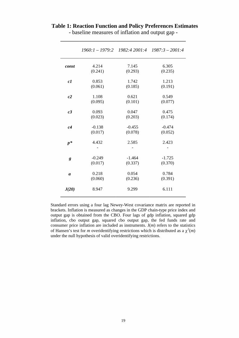
Table 1 reports the GMM estimates of the feedback coe¢cients as well as the relevant parame-

ters on asymmetric behavior for the baseline case corresponding to GDP chain-type in‡ation

and CBO output gap. The policy preferences ° and ®, which feature an asymmetric loss func-

tion, have the expected signs and they are marginally signi…cant throughout the table with

the exception of ® for the second subsample. A remarkable shift in output gap asymmetries

is observed between the pre- (…rst column) and the post-Volcker (second column) regimes in

that ° moves to an absolute value bigger than one in the latter period (we will return on the

third column in the following subsection). All feedback coe¢cients but the one on squared

in‡ation in the second subsample are signi…cantly di¤erent from zero and they allow us to

perform the crucial hypothesis testing of our analysis.

The …rst row of Table 2 shows that the null hypothesis of a linear reaction function, which

corresponds to the joint null of symmetric central bank preferences, is strongly rejected over

the two periods with the Wald statistics being much larger than the relevant critical value7

(disregard the last two columns for the time being). Lastly, it can be argued that potential5Notice that because no lagged interest rate terms appear in (7) as explanatory variable, the error component

is likely to be serially correlated. This is more that a standard error issue as it implies a violation of theorthogonality conditions stemming from the New-Keynesian transmission mechanism. We solve the issue byremoving from the set of instruments so many lags as to make the residuals nonsystematic. This amounts toreplace the …rst lag of each instrument in the pre-79 period and the …rst three lags in the post-79 period withtheir own earlier lags. An F-test applied to the …rst-stage regression rejects the hypothesis of weak instruments.

6 Indeed, under asymmetric central bank preferences the in‡ation conditional mean may be either below orabove the in‡ation target depending, inter alia, on the relative size of the policy parameters on in‡ation andoutput gaps (see Nobay and Peel, 1998, Ruge-Murcia, 2002, and Cukierman, 2001, for a formal derivation ofthis novel in‡ation bias). However, under the null of symmetric preferences such a bias disappears (i.e. averagein‡ation equals in‡ation target), thereby preserving the validity of our hypothesis testing strategy.

7The results are una¤ected by two robustness checks. The …rst uses F -versions of the Wald statistics asopposed to the Â2 variants which may be oversized in small samples. The second adds a cubic term for in‡ationand output gap as implied by a second-order Taylor expansion of the nonlinear policy rule.

11

measurement errors for the state variables are likely to a¤ect the point estimates of the

reaction function and most importantly the power of the test for the presence of nonlinearities.

However, Kuha and Temple (2002) show that measurement error in quadratic regression

tends to hide the presence of nonlinearities, thereby making stronger the case for asymmetric

preferences and suggesting that our estimates are better interpreted as a lower bound.

4.1.1 Comparison to other empirical estimates and subsample stability

It is useful at this point to compare our results with the empirical estimates obtained in

other recent studies in order to gauge their plausibility. In the pre-Volcker period, Clarida,

Galì and Gertler (2000) estimate a forward-looking linear reaction function with an ad-hoc

adjustment mechanism and …nd values of 0:83 for the coe¢cient on in‡ation (s.e.= 0:07)

and 0:27 for the coe¢cient on output (s.e.= 0:08). The signi…cant di¤erence comes from the

output gap parameter which suggests that neglecting the quadratic term, which enters our

empirical speci…cation with a negative sing, introduces a downward bias in the linear estimate.

Turning to a nonlinear speci…cation, Dolado, Maria-Dolores and Ruge-Murcia (2002) use a

Clarida, Galì and Gertler-type rule augmented with a generated regressor for the conditional

variance of in‡ation and estimate the marginal impact of in‡ation at 1:14 (s.e.= 0:12) and

the one of output at 0:31 (s.e.= 0:11). In addition to the downward bias for the output level,

their …ndings suggest that neglecting the quadratic terms introduce also an upward bias for

the coe¢cient on in‡ation level, which is consistent with the positive estimate we get for the

squared in‡ation.

The picture is completed by the post-Volcker estimates. Both coe¢cients on in‡ation

level and output level display di¤erences of expected sign relative to the values reported in

Clarida, Galì and Gertler (2000) while they are consistent with those provided by Dolado,

Maria-Dolores and Ruge-Murcia (2002). Lastly, we line up with early contributions in that

the coe¢cient on the in‡ation level becomes bigger than one moving from the pre- to the

post-Volcker era.

It should be noticed that as no lagged policy rate terms enter the nonlinear interest rate

rule (7), our estimates should be interpreted as long-run responses. Interestingly, they can

also be interpreted as short-run coe¢cients if one is willing to consider monetary policy inertia

as an illusion re‡ecting the episodic unforecastable persistent shocks that central banks face.

In this vein, Rudebusch (2002) use our baseline measure of in‡ation and output gap over

the period 1987:4-1999:4 to estimate with instrumental variables a linear forward-looking US

monetary policy rule which is all alike equation (7) but the squared variables. In order to

make our estimates directly comparable with those in Rudebusch (2002), we re-evaluate the

12

nonlinear policy rule over the Greenspan sample. In so doing, we can also assess the robustness

of our results to subsample stability.

The estimates are reported in the third column of Table 1 and they reinforce the …ndings

obtained so far. Indeed, not only all parameters are statistically di¤erent from zero and take

the expected sign but also the coe¢cient on in‡ation asymmetries becomes now signi…cant.

The value of ° keeps growing over time con…rming a signi…cant shift in the Fed output pref-

erences across the pre- and post-Volcker tenures, while the Wald statistics rejects the null of

symmetric preferences with a value of 83:883.

Turning to the comparison to other empirical estimates, we observe that neglecting the

squared variables introduces once more a signi…cant omitted variable bias. In particular, the

estimates provided in Rudebusch (2002) read the parameter on in‡ation levels at 2:00 (with s.e.

= 0:66) and the one on output gap levels at 0:39 (with s.e. = 0:24). By contrast, the results

we report in Table 1 shows that the point estimate of c1 is signi…cantly reduced whenever

the policy rule incorporates a squared in‡ation term whereas c2 becomes higher whenever a

squared output gap term is allowed for. While part of the di¤erences can be attributed to

both the longer sample and the non-annualized quarterly in‡ation we use, our results seem

to suggest a signi…cant role for the nonlinear components of US monetary policy rules. Such

a conclusion mirrors the estimates by Cukierman and Muscatelli (2002) who, employing an

ad-hoc speci…cation for the reaction function over a slightly longer sample, …nd a positive and

signi…cant coe¢cient for the nonlinear in‡ation term and a negative and signi…cant coe¢cient

for the nonlinear output component.

4.2 Robustness analysis

We assess now in turn the robustness of our …ndings to alternative measures of in‡ation and

output gap. Table 3 reports the estimates obtained with GMM using, everything equals,

the changes in the consumer price index as measure of in‡ation. All preference parameters

on asymmetries have the expected sign. In analogy to the results in Table 1, the coe¢cient

° on output gap displays a substantial growth over time in absolute values, although it is

less pronounced than for the GDP chain-type in‡ation. All reaction function coe¢cients are

signi…cant but c4 in the pre-Volcker period, which translates into a nonsigni…cant value of °.

The asymmetric preference parameter on in‡ation is still not statistically di¤erent from zero

over the second sample. Nevertheless, the Wald statistics displayed in the second row of Table

2 show that the joint null hypothesis of a linear policy rules is strongly rejected over both

samples.

We re-estimate the policy rule(7) using GDP chain-type in‡ation and detrended output

13

as measures of the state variables. The results are shown in Table 4 and they mirror those

of previous tables over the pre-79 regime. In particular, signi…cant values of the feedback

coe¢cients map into signi…cant values of the asymmetric parameters, which once more display

the expected signs. Turning to the post-Volcker period, a di¤erent picture emerges. While

the preference parameter ° is still negative and signi…cant and con…rms in absolute values its

growing path over time, the coe¢cient ® on in‡ation asymmetries takes now a negative and

signi…cant value. However, the relevance of the latter result has to be weighted by the fact

that detrended output may be not an appropriate measure of the business cycle.8

We complete the robustness analysis by introducing an interest rate smoothing argument

into the nonlinear policy rule to evaluate whether the Fed tendency to smooth policy rates

may turn out to be responsible for a seemingly nonlinear behavior.9 The estimates of the

policy preferences line up with those of the baseline case while the last row of Table 2 shows

that the null of symmetric preferences is once more strongly rejected over both samples. This

…nding suggests that squared in‡ation and squared output gap capture a genuine nonlinear

behavior and therefore they have a place on their own right in US monetary policy rules.10

4.3 Discussion

A number of di¤erent results stem from the estimates reported above. On the one hand,

the preference parameter on output asymmetries, whose identi…cation does not require any

additional assumption on the model coe¢cients, takes negative and signi…cant values. Such

an evidence is robust across alternative measures of in‡ation and output gaps being consistent

with an asymmetric speci…cation of the central bank objectives. In addition, the signi…cant

increase of ° over time appears to be a robust feature of the data corroborating the view

that a regime shift has occurred between the pre- and the post-1979 Chairmen. On the other

hand, the estimates on the in‡ation preference parameter, ®, take a positive sign and they

are signi…cantly di¤erent from zero mainly over the …rst sample.

These …ndings enrich the picture provided by Clarida, Galì and Gertler (2000) and indicate

that nonlinearity has signi…cantly characterized the postwar policy stance of the Fed. Indeed,

equation (7) makes clear that under asymmetric preferences the interest rate responses are8 Indeed, as argued by McCallum and Nelson (1999), not only the …tted trend displays a signi…cantly more

volatile path than the CBO time series, especially during the post-Volcker period, but also it does not capturethe conventional wisdom that output has been unusually high relative to potential in the mid-90s.

9Estimates of the reaction function and the preference parameters in the presence of interest rate smoothingare not reported here to save space, but they are available from the author upon request.

10Surico (2002) shows that these results are robust to both a backward-looking structure of the economy àla Rudebusch and Svensson (1999) and to a nonparametric speci…cation of the central bank loss function. Inparticular, the nonparametric estimates suggest that the nonlinearities found in US monetary policy rules areconsistent with an objective function that is both nonquadratic and asymmetric.

14

not anymore time invariant but rather they depend on the level of in‡ation and output

gaps. Accordingly, large deviations of the target variables require vigorous movements of

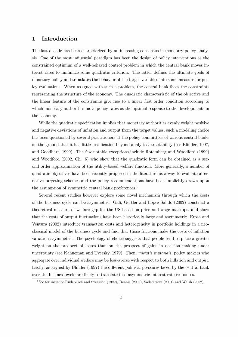
policy rates whereas small deviations require only limited changes. This point is illustrated

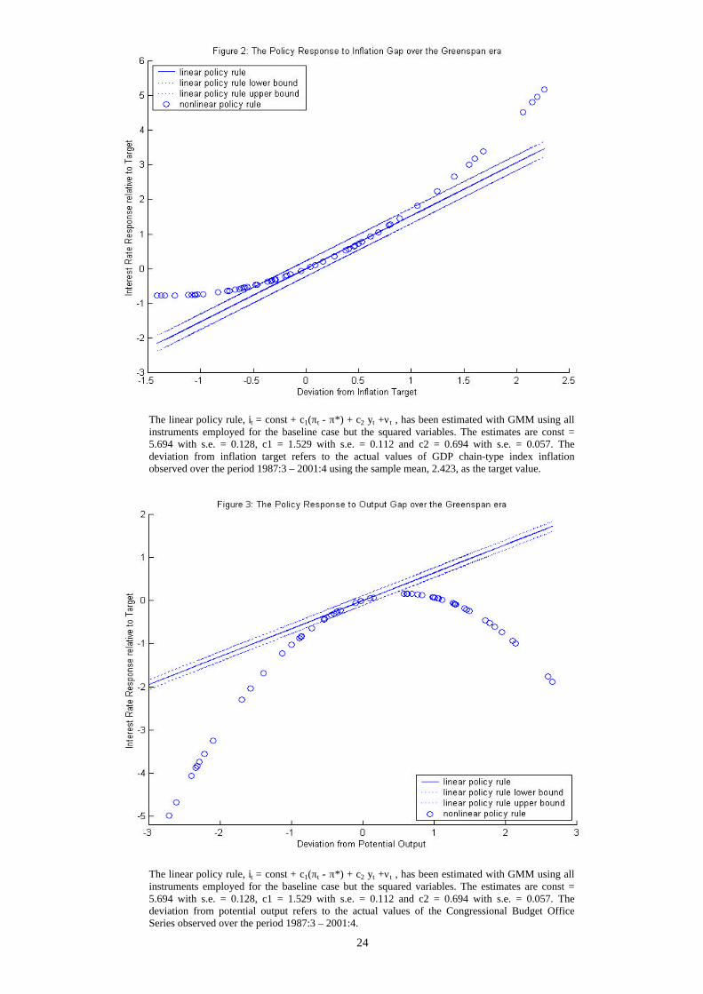
in Figure 2 and 3 which compare our baseline estimates with those obtained using a linear

speci…cation of the policy rule (i.e. forcing c3 and c4 to be zero). The vertical axis displays

the interest rate responses (relative to target) implied by the estimates of the two rules while

the horizontal axis reports the actual movements over the Greenspan sample for in‡ation

and output gaps respectively. The graphs show not only that US monetary policy has been

signi…cantly nonlinear and asymmetric but also that large gaps have been penalized more

than small gaps with the exception of the negative deviations of in‡ation.

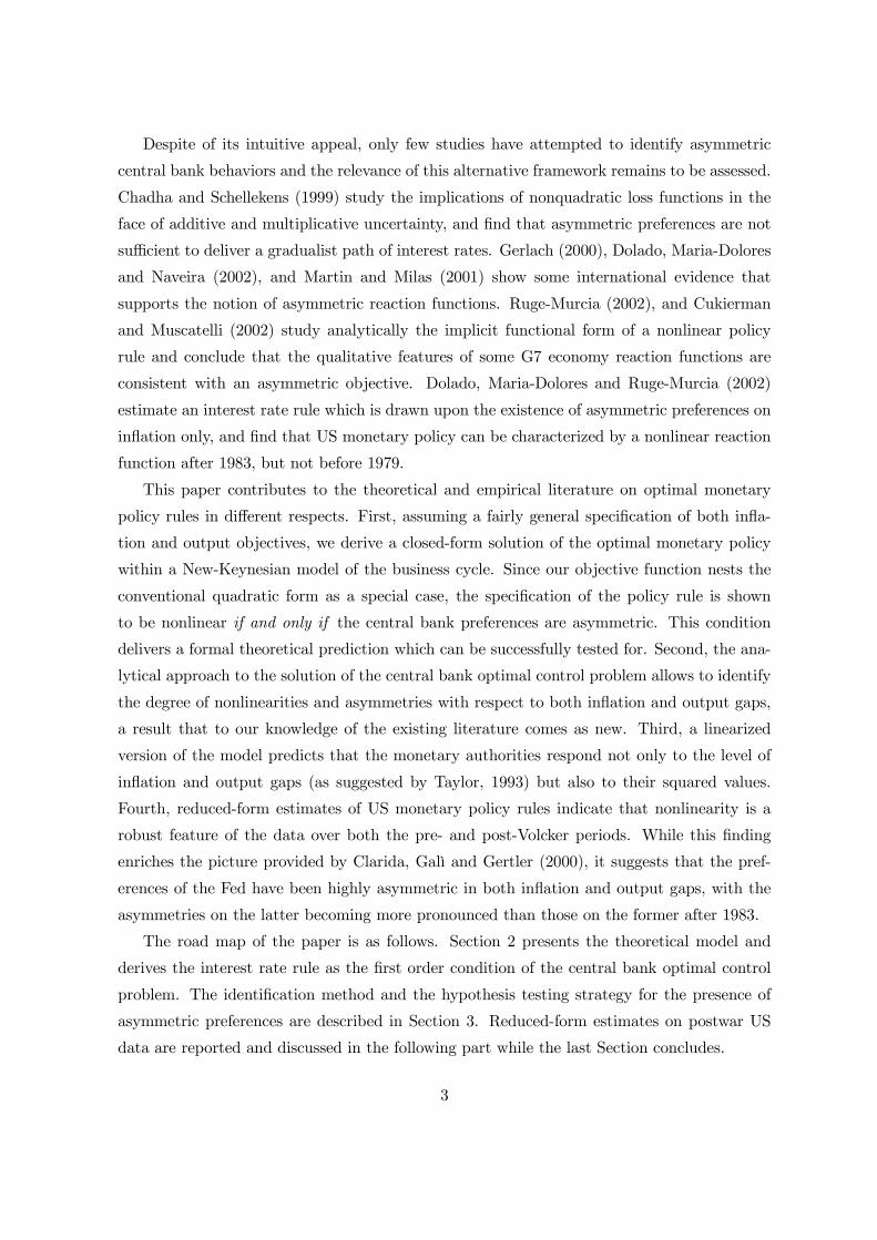
Furthermore, Figure 3 shows that only according to the nonlinear policy rule interest rates

have been lowered in response to both positive and negative output gaps with the former

mostly corresponding to the period 1997:1-2001:1. Interestingly, this observation is consistent

with the view that the Fed has taken advantage of the benign macroeconomic conditions of

the late 90s to accommodate the favorable supply shocks that the ’New Economy’ has brought

about.11 It should be noticed that the reversed U-shape policy response displayed in Figure 3

is a feature of the post-Volcker era only since over the …rst sample the relative size of c2 over

c4 is considerably higher in absolute value than its post-79 counterpart (see Table 1). Indeed,

while the squared term translates into a signi…cant asymmetric behavior also over the pre-79

sample, the coe¢cient on levels, which is now bigger than one, makes the nonlinear relation

between interest rates and output gap positive over the entire domain.

Lastly, a comparison of ® and ° across samples shows that output asymmetries have be-

come relatively more pronounced during the post-Volcker tenures. In particular, the presence

of highly asymmetric preferences on output seems to rationalize the sequences of downwards

movements through which the Fed has considerably cut interest rates during 2001.

5 Conclusions

The contribution of this paper is twofold. At the theoretical level it derives a general closed-

form solution for interest rate rules when central bank preferences are asymmetric in both

in‡ation and output gaps, and the monetary transmission mechanism is New-Keynesian. The

speci…cation of the policy objectives nests the quadratic form as a special case and therefore11Notice that by using the (CBO) output gap as opposed to the unemployment rate we have implicitely

speci…ed a time-varying target for the stabilization of the business cycle. Moreover, since the potential outputseries is constructed upon revised data, the argument that a shift in the NAIRU estimates may have warrantedsuch a seemingly nonlinear behavior does not apply here.

15

it translates into a potentially nonlinear monetary policy rule. This modeling feature forms

the basis of our hypothesis testing strategy for the presence of asymmetric preferences as it

allows to reversely engineer potential evidence of nonlinearities in the reaction functions into

evidence of asymmetries in the policy objectives.

At the empirical level this paper shows that US monetary policy can be characterized

by a nonlinear policy rule during both the pre- and post-Volcker eras, with the interest rate

responses to the state of the business cycle being the dominant form of nonlinearity over the

second sample. Moreover, our identi…cation method indicates that the preferences of the Fed

have been highly asymmetric with respect to both in‡ation and output gaps, and that the

asymmetries on the latter have become relatively more pronounced after 1983. These …ndings

are robust across alternative measures of in‡ation and output gap as well as to the existence

of an interest rate smoothing goal in the central bank loss function.

Altogether, this paper develops a formal hypothesis testing for the presence of asymmetric

preferences. As the null of the test features the quadratic form used in earlier contributions, our

results suggest some caution about using symmetric loss functions as a guide to policy analysis.

Indeed, promising strands of literature have recently emphasized that labor market frictions

and heterogeneity in portfolio holdings can make the welfare costs of business ‡uctuations and

in‡ation asymmetric. Along these lines, a stimulating avenue for future research is to derive

an utility-based welfare function within richer models of the business cycle in order to provide

a formal microfoundation for an asymmetric central bank objective. The proposal by Geraats

(1999) comes as an intriguing step in this direction.

16

ReferencesBarro, R.J. and D. Gordon, 1983, A Positive Theory of Monetary Policy in a Natural Rate

Model, Journal of Political Economy 91, 589-610.

Bernanke, B. and I. Mihov, 1998, Measuring Monetary Policy, Quarterly Journal of Eco-nomics 63, 869-902.

Blinder, A., 1997, Distinguished Lecture on Economics and Government: What CentralBankers Could Learn from Academics and Viceversa, Journal of Economic Perspective11, 3-19.

Chadha, J.S. and P. Schellekens, 1999, Monetary policy loss functions: two cheers for thequadratic, DAE Working Paper 99/20.

Clarida, R., J. Galì and M. Gertler, 2000, Monetary Policy Rules and Macroeconomic Sta-bility: Evidence and Some Theory, Quarterly Journal of Economics 115, 147-180.

Clarida, R., J. Galì and M. Gertler, 1999, The Science of Monetary Policy: A New KeynesianPerspective, Journal of Economic Literature 37, 1661-1707.

Cukierman, A, and V.A. Muscatelli, 2002, Do Central Banks have Precautionary Demandsfor Expansions and for Price Stability? - Theory and Evidence, mimeo, Tel-Aviv Uni-versity.

Cukierman, A., 2001, The In‡ation Bias Result Revisited, mimeo, Tel-Aviv University.

Dennis, R., 2002, The Policy Preferences of the US Federal Reserve. Federal Reserve of SanFrancisco Working paper No. 2001-08.

Dolado, J.J., R. Maria-Dolores and M. Naveira, 2002, Are Monetary-Policy Reaction Func-tions Asymmetric? The Role of Nonlinearity in the Phillips Curve, mimeo, UniversidadCarlos III de Madrid.

Dolado, J.J., R. Maria-Dolores and F.J. Ruge-Murcia, 2002, Nonlinear Monetary PolicyRules: Some New Evidence for the US, CEPR Discussion paper No. 3405.

Erosa, A. and G. Ventura, 2002, On In‡ation as a Regressive Consumption Tax, Journal ofMonetary Economics 49, 761-795.

Galì, J., M. Gertler and J.D. Lopez-Salido, 2002, Markups, Gaps, and the Welfare Costs ofBusiness Fluctuations, mimeo, Universitat Pompeu Fabra.

Geraats, P., 1999, In‡ation and Its Variation: An Alternative Explanation, CIDER WorkingPaper C99-105.

Gerlach, S., 2000, Asymmetric Policy Reactions and In‡ation, mimeo, BIS.

Goodhart, C.A.E., 1999, Central Bank and Uncertainty, Bank of England Quarterly BulletinFebruary, 102-121.

Granger, C.W.J. and T. Teräsvirta 1993, Modelling Non-linear Economic Relationship, (Ox-ford University Press).

Hansen, L.P., 1982, Large Sample Properties of Generalized Method of Moments Estimators.Econometrica 50, 1029-1054.

17

Judd, J.P. and G.D. Rudebusch, 1998, Taylor’s rule and the Fed: 1970-1997, Federal ReserveBank of San Francisco, Economic Review 3, 3-16.

Kahneman, D. and A., Tversky, 1979, Prospect Theory: An Analysis of Decision under Risk,Econometrica 47, 263-292.

Kuha, J. and J. Temple, 2002, Covariate Measurement Error in Quadratic Regression, mimeo,University of Bristol.

Martin, C. and C. Milas, 2001, Modelling Monetary Policy: In‡ation Targeting in Practice,mimeo, Brunel University.

McCallum, B. and E. Nelson, 1999, Performance of Operational Policy Rules in an EstimatedSemiclassical Structural Model, in: Taylor, J.B., ed., Monetary Policy Rules, (ChicagoUniversity press).

Nobay, R. and D. Peel, 1998, Optimal Monetary Policy in a Model of Asymmetric CentralBank Preferences, mimeo, London School of Economics.

Rotemberg, J.J. and M. Woodford, M., 1999, Interest Rate Rules in an Estimated StickyPrice Model, in: Taylor, J.B., ed., Monetary Policy Rules, (Chicago University press).

Rudebusch, G.D., 2002, Term Structure Evidence on Interest Rate Smoothing and MonetaryPolicy Inertia, Journal of Monetary Economics 49, 1161-1187.

Rudebusch, G.D. and L.E.O. Svensson, 1999, Policy Rules for In‡ation Targeting, in: Taylor,J.B., ed., Monetary Policy Rules, (Chicago University press).

Ruge-Murcia, F.J., 2002, The In‡ation Bias when the Central Banker Targets the NaturalRate of Unemployment, European Economic Review, forthcoming.

Söderström, U., 2001, Targeting In‡ation with a Prominent Role for Money, Sveriges Riks-bank working Paper No. 123.

Surico, P., 2002. Asymmetric Central Bank Preferences and Nonlinear Policy Rules, BocconiUniversity working paper EEA 02-5.

Svensson, L.E.O., 1999, In‡ation Targeting as a Monetary Policy Rule, Journal of MonetaryEconomics, 43, 607-654.

Taylor, J.B., 1993, Discretion versus Policy Rules in Practice, Carnegie-Rochester conferenceseries on public policy 39, 195-214.

Varian, H., 1974, A Bayesian Approach to Real Estate Assessment, in: Feinberg, S.E., and A.Zellner, eds., Studies in Bayesian Economics in Honour of L.J. Savage (North Holland).

Walsh, C., 2002, Speed Limit Policies: The Output Gap and Optimal Monetary Policy,American Economic Review, forthcoming.

Woodford, M., 2002, Interest and Prices: Foundations of a Theory of Monetary Policy,forthcoming, (Princeton University Press).

Yun, T., 1996, Nominal Price Rigidity, Money Supply Endogeneity, and Business Cycles,Journal of Monetary Economics 37, 345-370.

Zellner, A., 1986, Bayesian Estimation and Prediction Using Asymmetric Loss Functions,Journal of the American Statistical Association 81, 446-451.

18

19

Table 1: Reaction Function and Policy Preferences Estimates- baseline measures of inflation and output gap -

1960:1 – 1979:2 1982:4 2001:4 1987:3 – 2001:4

const 4.214(0.241)

7.145(0.293)

6.305(0.235)

c1 0.853(0.061)

1.742(0.185)

1.213(0.191)

c2 1.108(0.095)

0.621(0.101)

0.549(0.077)

c3 0.093(0.023)

0.047(0.203)

0.475(0.174)

c4 -0.138(0.017)

-0.455(0.078)

-0.474(0.052)

π* 4.432-

2.585-

2.423-

γ -0.249(0.017)

-1.464(0.337)

-1.725(0.370)

α 0.218(0.060)

0.054(0.236)

0.784(0.391)

J(20) 8.947 9.299 6.111

Standard errors using a four lag Newey-West covariance matrix are reported inbrackets. Inflation is measured as changes in the GDP chain-type price index andoutput gap is obtained from the CBO. Four lags of gdp inflation, squared gdpinflation, cbo output gap, squared cbo output gap, the fed funds rate andconsumer price inflation are included as instruments. J(m) refers to the statisticsof Hansen’s test for m overidentifying restrictions which is distributed as a χ2(m)under the null hypothesis of valid overidentifying restrictions.

20

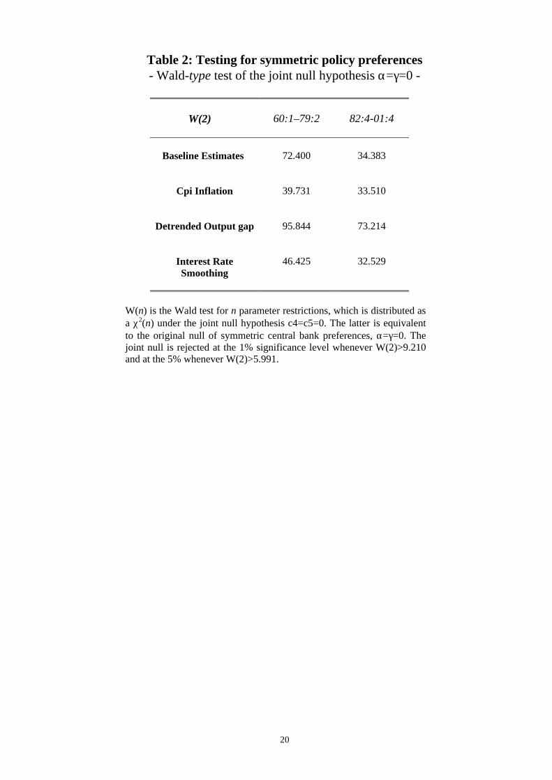
Table 2: Testing for symmetric policy preferences- Wald-type test of the joint null hypothesis α=γ=0 -

W(2) 60:1–79:2 82:4-01:4

Baseline Estimates 72.400 34.383

Cpi Inflation 39.731 33.510

Detrended Output gap 95.844 73.214

Interest RateSmoothing

46.425 32.529

W(n) is the Wald test for n parameter restrictions, which is distributed asa χ2(n) under the joint null hypothesis c4=c5=0. The latter is equivalentto the original null of symmetric central bank preferences, α=γ=0. Thejoint null is rejected at the 1% significance level whenever W(2)>9.210and at the 5% whenever W(2)>5.991.

21

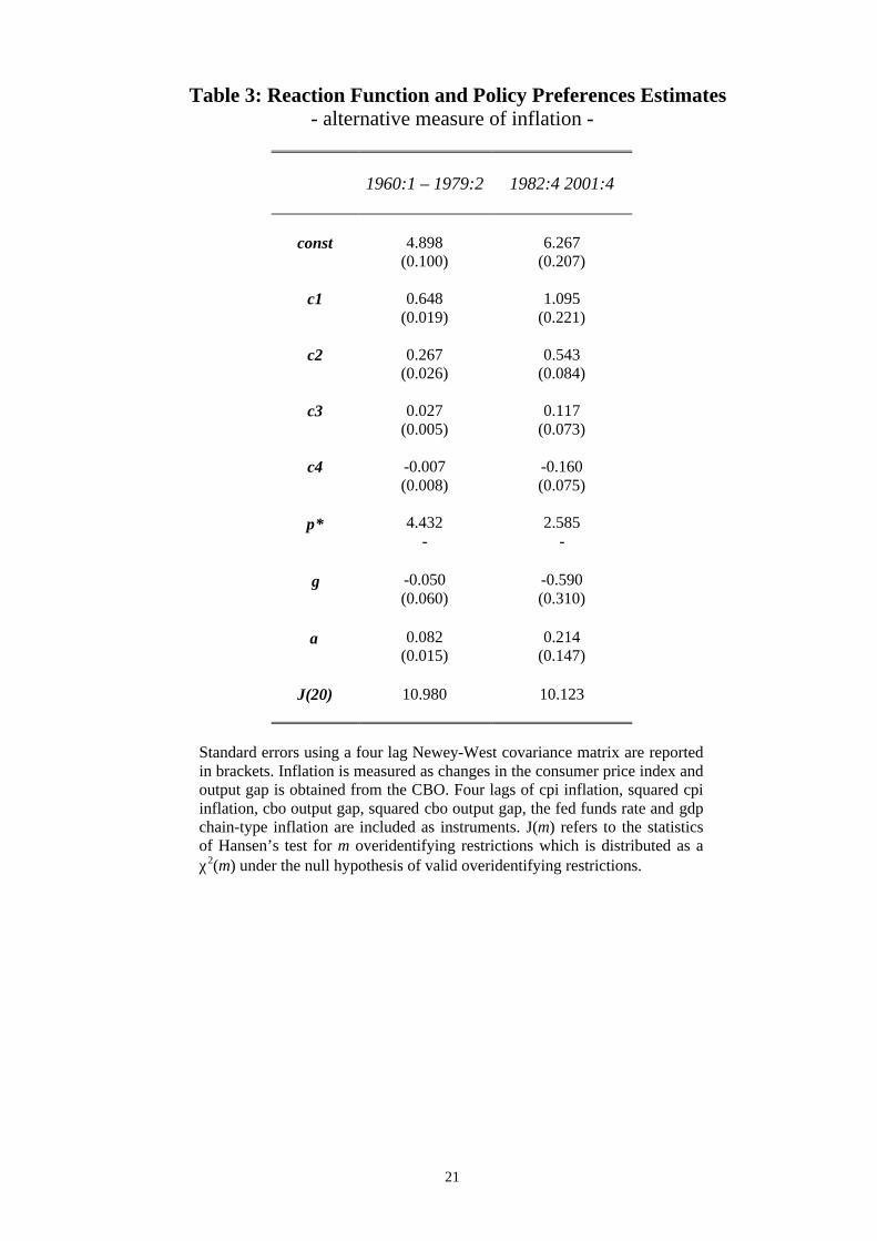
Table 3: Reaction Function and Policy Preferences Estimates- alternative measure of inflation -

1960:1 – 1979:2 1982:4 2001:4

const 4.898(0.100)

6.267(0.207)

c1 0.648(0.019)

1.095(0.221)

c2 0.267(0.026)

0.543(0.084)

c3 0.027(0.005)

0.117(0.073)

c4 -0.007(0.008)

-0.160(0.075)

π* 4.432-

2.585-

γ -0.050(0.060)

-0.590(0.310)

α 0.082(0.015)

0.214(0.147)

J(20) 10.980 10.123

Standard errors using a four lag Newey-West covariance matrix are reportedin brackets. Inflation is measured as changes in the consumer price index andoutput gap is obtained from the CBO. Four lags of cpi inflation, squared cpiinflation, cbo output gap, squared cbo output gap, the fed funds rate and gdpchain-type inflation are included as instruments. J(m) refers to the statisticsof Hansen’s test for m overidentifying restrictions which is distributed as aχ2(m) under the null hypothesis of valid overidentifying restrictions.

22

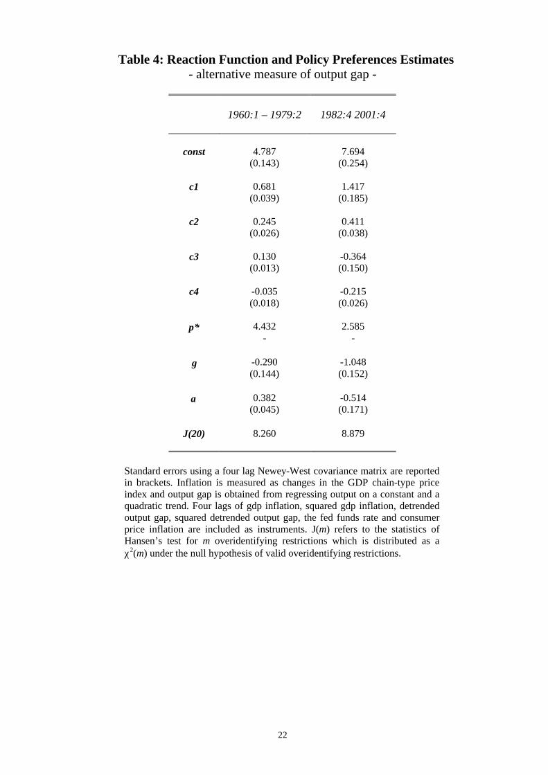
Table 4: Reaction Function and Policy Preferences Estimates- alternative measure of output gap -

1960:1 – 1979:2 1982:4 2001:4

const 4.787(0.143)

7.694(0.254)

c1 0.681(0.039)

1.417(0.185)

c2 0.245(0.026)

0.411(0.038)

c3 0.130(0.013)

-0.364(0.150)

c4 -0.035(0.018)

-0.215(0.026)

π* 4.432-

2.585-

γ -0.290(0.144)

-1.048(0.152)

α 0.382(0.045)

-0.514(0.171)

J(20) 8.260 8.879

Standard errors using a four lag Newey-West covariance matrix are reportedin brackets. Inflation is measured as changes in the GDP chain-type priceindex and output gap is obtained from regressing output on a constant and aquadratic trend. Four lags of gdp inflation, squared gdp inflation, detrendedoutput gap, squared detrended output gap, the fed funds rate and consumerprice inflation are included as instruments. J(m) refers to the statistics ofHansen’s test for m overidentifying restrictions which is distributed as aχ2(m) under the null hypothesis of valid overidentifying restrictions.

23

24

The linear policy rule, it = const + c1(πt - π*) + c2 yt +νt , has been estimated with GMM using allinstruments employed for the baseline case but the squared variables. The estimates are const =5.694 with s.e. = 0.128, c1 = 1.529 with s.e. = 0.112 and c2 = 0.694 with s.e. = 0.057. Thedeviation from inflation target refers to the actual values of GDP chain-type index inflationobserved over the period 1987:3 – 2001:4 using the sample mean, 2.423, as the target value.

The linear policy rule, it = const + c1(πt - π*) + c2 yt +νt , has been estimated with GMM using allinstruments employed for the baseline case but the squared variables. The estimates are const =5.694 with s.e. = 0.128, c1 = 1.529 with s.e. = 0.112 and c2 = 0.694 with s.e. = 0.057. Thedeviation from potential output refers to the actual values of the Congressional Budget OfficeSeries observed over the period 1987:3 – 2001:4.