SLAC-RF: Simultaneous 3D Localization of mobile

readers and Calibration of RFID supertags

Venkatesan EkambaramKannan Ramchandran

Electrical Engineering and Computer SciencesUniversity of California at Berkeley

Technical Report No. UCB/EECS-2012-188

http://www.eecs.berkeley.edu/Pubs/TechRpts/2012/EECS-2012-188.html

August 18, 2012

Copyright © 2012, by the author(s).All rights reserved.

Permission to make digital or hard copies of all or part of this work forpersonal or classroom use is granted without fee provided that copies arenot made or distributed for profit or commercial advantage and that copiesbear this notice and the full citation on the first page. To copy otherwise, torepublish, to post on servers or to redistribute to lists, requires prior specificpermission.

1

SLAC-RF: Simultaneous 3D Localization of mobile

readers And Calibration of RFID supertagsVenkatesan. N. Ekambaram, Kannan Ramchandran

Department of EECS, University of California, Berkeley

Email: {venkyne@eecs.berkeley.edu, kannanr@eecs.berkeley.edu}

Abstract

We propose a novel and inexpensive infrastructure for precise localization in non-line-of-sight wireless environ-

ments using RFID tags. The proposed system utilizes specialized tags that we term as supertags. Each supertag is

an array of individual single antenna RFID tags closely spaced so as to emulate a “virtual” antenna array. Multiple

such supertags are installed in a 3D environment where we are interested in localizing mobile agents equipped with

an RFID reader. Only a small fraction of the supertags are assumed to be calibrated in terms of their location and

orientation. We develop signal processing algorithms to precisely estimate the location of the mobile reader and

simultaneously calibrate the supertags. The goal is to design an inexpensive and precise localization system that is

robust to non-line-of-sight errors, and which does not require careful placement of anchors in the environment. We

show through simulations that it is possible to obtain highly accurate estimates of the mobile reader’s location even

in a multipath rich environment, and that the supertags get calibrated over time as multiple mobile readers pass

through the environment.

I. INTRODUCTION

Precise localization is of interest in many applications such as for safety in vehicular networks [1], indoor

localization [2], 3D modeling and navigation inside buildings [3] etc. Certain military applications require unmanned

air vehicles (UAVs) navigate in unfamiliar environments [4]. GPS is significantly affected by non-line-of-sight

(NLOS) propagation in environments like urban canyons and is unavailable for indoor applications. Multipath

propagation degrades the signal quality and further introduces large bias errors in the measurements that lead to

highly imprecise location estimates. Many system architectures have been proposed in the literature that address the

problem of NLOS localization, in particular for indoor localization. Companies like Qualcomm, Nokia, Microsoft,

Ericsson, Google, Locata etc, have developed both software and hardware for indoor localization applications.

This project is supported in part by an AFOSR grant (FA9550-10-1-0567).

2

!"#$%&'()*+,-.%

/0123)%*),4)*5,-)6+%

7,89.8,:)*)4%%.2-6,3.%

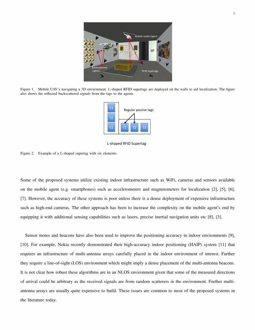
Figure 1. Mobile UAV’s navigating a 3D environment. L-shaped RFID supertags are deployed on the walls to aid localization. The figurealso shows the reflected backscattered signals from the tags to the agents.!"#$%&'()*+,-.%

/0123)%,-)4+%!)5)6+)7%1,68.6,9)*%

%.2-4,3.%%

:;%

:<%

:=% :;%:<%:=%

>?.@,()7%!"#$%&'()*+,-%

!)-'3,*%(,..2A)%+,-.%

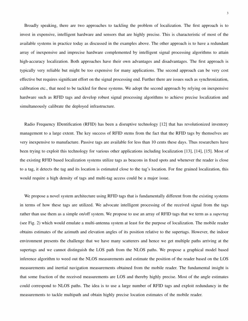
Figure 2. Example of a L-shaped supertag with six elements.

Some of the proposed systems utilize existing indoor infrastructure such as WiFi, cameras and sensors available

on the mobile agent (e.g. smartphones) such as accelerometers and magnetometers for localization [2], [5], [6],

[7]. However, the accuracy of these systems is poor unless there is a dense deployment of expensive infrastructure

such as high-end cameras. The other approach has been to increase the complexity on the mobile agent’s end by

equipping it with additional sensing capabilities such as lasers, precise inertial navigation units etc [8], [3].

Sensor motes and beacons have also been used to improve the positioning accuracy in indoor environments [9],

[10]. For example, Nokia recently demonstrated their high-accuracy indoor positioning (HAIP) system [11] that

requires an infrastructure of multi-antenna arrays carefully placed in the indoor environment of interest. Further

they require a line-of-sight (LOS) environment which might imply a dense placement of the multi-antenna beacons.

It is not clear how robust these algorithms are in an NLOS environment given that some of the measured directions

of arrival could be arbitrary as the received signals are from random scatterers in the environment. Further multi-

antenna arrays are usually quite expensive to build. These issues are common to most of the proposed systems in

the literature today.

3

Broadly speaking, there are two approaches to tackling the problem of localization. The first approach is to

invest in expensive, intelligent hardware and sensors that are highly precise. This is characteristic of most of the

available systems in practice today as discussed in the examples above. The other approach is to have a redundant

array of inexpensive and imprecise hardware complemented by intelligent signal processing algorithms to attain

high-accuracy localization. Both approaches have their own advantages and disadvantages. The first approach is

typically very reliable but might be too expensive for many applications. The second approach can be very cost

effective but requires significant effort on the signal processing end. Further there are issues such as synchronization,

calibration etc., that need to be tackled for these systems. We adopt the second approach by relying on inexpensive

hardware such as RFID tags and develop robust signal processing algorithms to achieve precise localization and

simultaneously calibrate the deployed infrastructure.

Radio Frequency IDentification (RFID) has been a disruptive technology [12] that has revolutionized inventory

management to a large extent. The key success of RFID stems from the fact that the RFID tags by themselves are

very inexpensive to manufacture. Passive tags are available for less than 10 cents these days. Thus researchers have

been trying to exploit this technology for various other applications including localization [13], [14], [15]. Most of

the existing RFID based localization systems utilize tags as beacons in fixed spots and whenever the reader is close

to a tag, it detects the tag and its location is estimated close to the tag’s location. For fine grained localization, this

would require a high density of tags and multi-tag access could be a major issue.

We propose a novel system architecture using RFID tags that is fundamentally different from the existing systems

in terms of how these tags are utilized. We advocate intelligent processing of the received signal from the tags

rather than use them as a simple on/off system. We propose to use an array of RFID tags that we term as a supertag

(see Fig. 2) which would emulate a multi-antenna system at least for the purpose of localization. The mobile reader

obtains estimates of the azimuth and elevation angles of its position relative to the supertags. However, the indoor

environment presents the challenge that we have many scatterers and hence we get multiple paths arriving at the

supertags and we cannot distinguish the LOS path from the NLOS paths. We propose a graphical model based

inference algorithm to weed out the NLOS measurements and estimate the position of the reader based on the LOS

measurements and inertial navigation measurements obtained from the mobile reader. The fundamental insight is

that some fraction of the received measurements are LOS and thereby highly precise. Most of the angle estimates

could correspond to NLOS paths. The idea is to use a large number of RFID tags and exploit redundancy in the

measurements to tackle multipath and obtain highly precise location estimates of the mobile reader.

4

!"#$%&'()'*)+##",-.)

/0&1-2'#)

3$-4$#)5'%-&'()/0&1-2'#)

678$#2-9):-.";#-2'#))

<'4$.)8-#-1$2$#)$0&1-2'#0)

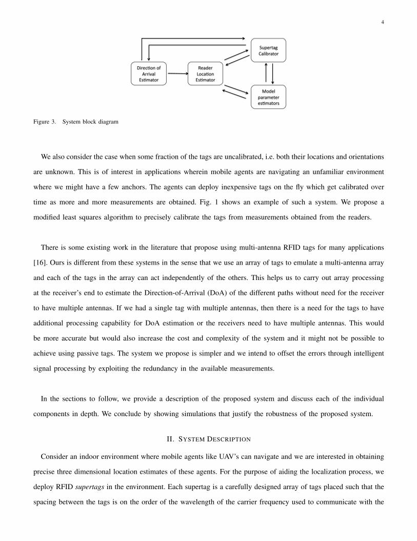
Figure 3. System block diagram

We also consider the case when some fraction of the tags are uncalibrated, i.e. both their locations and orientations

are unknown. This is of interest in applications wherein mobile agents are navigating an unfamiliar environment

where we might have a few anchors. The agents can deploy inexpensive tags on the fly which get calibrated over

time as more and more measurements are obtained. Fig. 1 shows an example of such a system. We propose a

modified least squares algorithm to precisely calibrate the tags from measurements obtained from the readers.

There is some existing work in the literature that propose using multi-antenna RFID tags for many applications

[16]. Ours is different from these systems in the sense that we use an array of tags to emulate a multi-antenna array

and each of the tags in the array can act independently of the others. This helps us to carry out array processing

at the receiver’s end to estimate the Direction-of-Arrival (DoA) of the different paths without need for the receiver

to have multiple antennas. If we had a single tag with multiple antennas, then there is a need for the tags to have

additional processing capability for DoA estimation or the receivers need to have multiple antennas. This would

be more accurate but would also increase the cost and complexity of the system and it might not be possible to

achieve using passive tags. The system we propose is simpler and we intend to offset the errors through intelligent

signal processing by exploiting the redundancy in the available measurements.

In the sections to follow, we provide a description of the proposed system and discuss each of the individual

components in depth. We conclude by showing simulations that justify the robustness of the proposed system.

II. SYSTEM DESCRIPTION

Consider an indoor environment where mobile agents like UAV’s can navigate and we are interested in obtaining

precise three dimensional location estimates of these agents. For the purpose of aiding the localization process, we

deploy RFID supertags in the environment. Each supertag is a carefully designed array of tags placed such that the

spacing between the tags is on the order of the wavelength of the carrier frequency used to communicate with the

5

tags. Thus the tags can essentially act as a multi-antenna array. For example, the tags could be arranged in a linear

L-shaped array (see Fig. 6) or in a circular architecture etc. Supertag architecture is in itself an important design

question which we do not address here. Our goal here is to evaluate the concept of using supertags for precise

localization. We assume a simple L-shaped tag array in our simulations. However, the theory and algorithms are

developed for a generic supertag architecture.

We assume that only some fraction of the tags are calibrated, i.e. known locations and orientations and the rest

are not. The goal is to simultaneously estimate the location of a mobile reader that navigates the environment and

calibrate the supertags. We assume that the mobile reader has a single antenna that transmits a carrier wave and

receives the backscattered signals from the tags which can be passive.

We need a mechanism by which the reader can distinguish the signals backscattered from each of the tags

individually. There are many MAC layer arbitration algorithms that have been proposed and are part of the

EPCGlobal Gen-2 RFID standard [17]. We assume a spread spectrum RFID system [18] based on CDMA codes

wherein each tag in the supertag modulates the received carrier signal with a unique CDMA code. These CDMA

codes can be spatially reused for different tags. This allows for a simpler system design and processing.

The high level operation of the system is based on localization using DoA measurements. The mobile reader

transmits a carrier wave that is backscatter modulated by the supertags in the vicinity of the reader. The design of

the supertag enables it to behave as a multi-antenna system and hence the reader which is assumed to only have a

single antenna can estimate the elevation and azimuth angles of arrival from each of the supertags in its vicinity.

Based on these measurements, the location of the mobile reader needs to be estimated. There are two challenges

here. Firstly, the locations and orientations of some of the supertags are not known or only known approximately.

Secondly, the environment is highly prone to multipath interference. Hence the estimated angles of arrival from the

supertags need not be the true azimuth and elevation angles of the supertag with respect to the reader. Only some

fraction of the measurements can be assumed to be true LOS angle estimates, though we do not know which of

them are. We develop algorithms that are robust to such NLOS noise.

In order to tackle the problem, we adopt a modular approach for the system design. A basic system block

diagram is shown in Fig. 3. The DoA estimator block outputs a set of azimuth and elevation angle estimates for

different paths corresponding to every supertag in the vicinity of the mobile reader. The reader location estimator

6

� kTc

(k−1)Tc

� kTc

(k−1)Tc

� kTc

(k−1)Tc

!"#$%&

#'()*+,-&$.&

CDMA 1

CDMA 2

CDMA L

g1

g2

gP

g1

g2

gP

CDMA 1

CDMA 2

CDMA L

∆1

∆2

∆P

∆1

∆2

∆P

δ11

δ12

δ1P

δ2P

δ3P

δ32

δ31

δ22

δ21

δ11

δ12

δ1P

δ21

δ22

δ2P

δ31

δ32

δ3P

!"##$%#&

!"##$%#&

/01&23##&4$/+56&

'#"()*$+%#&,-./0&-%"1%#2&

.3#4"#1&!5"((%6&-./0&789%#&'":&

-%;%$<%#&1%*3186"=3#&,-./0&-%"1%#2&

-%<%#)%&;5"((%6&

�

n

cks(t − nTc)

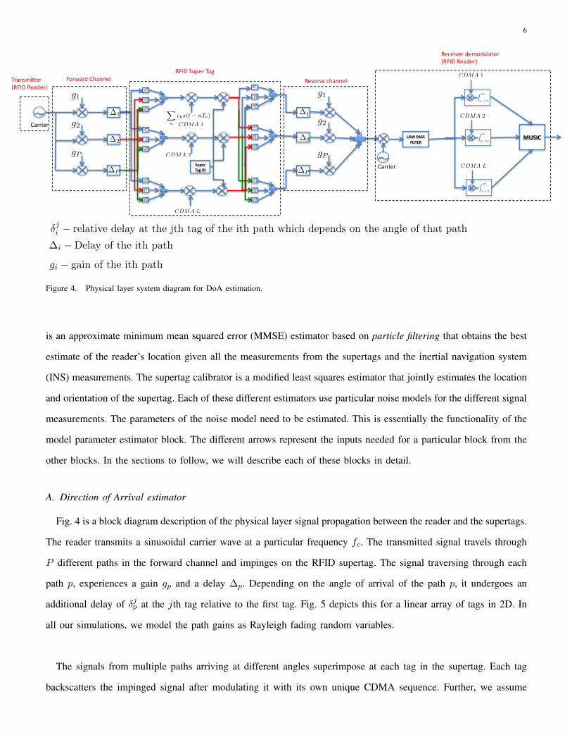
δji − relative delay at the jth tag of the ith path which depends on the angle of that path

∆i − Delay of the ith path

gi − gain of the ith path

Figure 4. Physical layer system diagram for DoA estimation.

is an approximate minimum mean squared error (MMSE) estimator based on particle filtering that obtains the best

estimate of the reader’s location given all the measurements from the supertags and the inertial navigation system

(INS) measurements. The supertag calibrator is a modified least squares estimator that jointly estimates the location

and orientation of the supertag. Each of these different estimators use particular noise models for the different signal

measurements. The parameters of the noise model need to be estimated. This is essentially the functionality of the

model parameter estimator block. The different arrows represent the inputs needed for a particular block from the

other blocks. In the sections to follow, we will describe each of these blocks in detail.

A. Direction of Arrival estimator

Fig. 4 is a block diagram description of the physical layer signal propagation between the reader and the supertags.

The reader transmits a sinusoidal carrier wave at a particular frequency fc. The transmitted signal travels through

P different paths in the forward channel and impinges on the RFID supertag. The signal traversing through each

path p, experiences a gain gp and a delay ∆p. Depending on the angle of arrival of the path p, it undergoes an

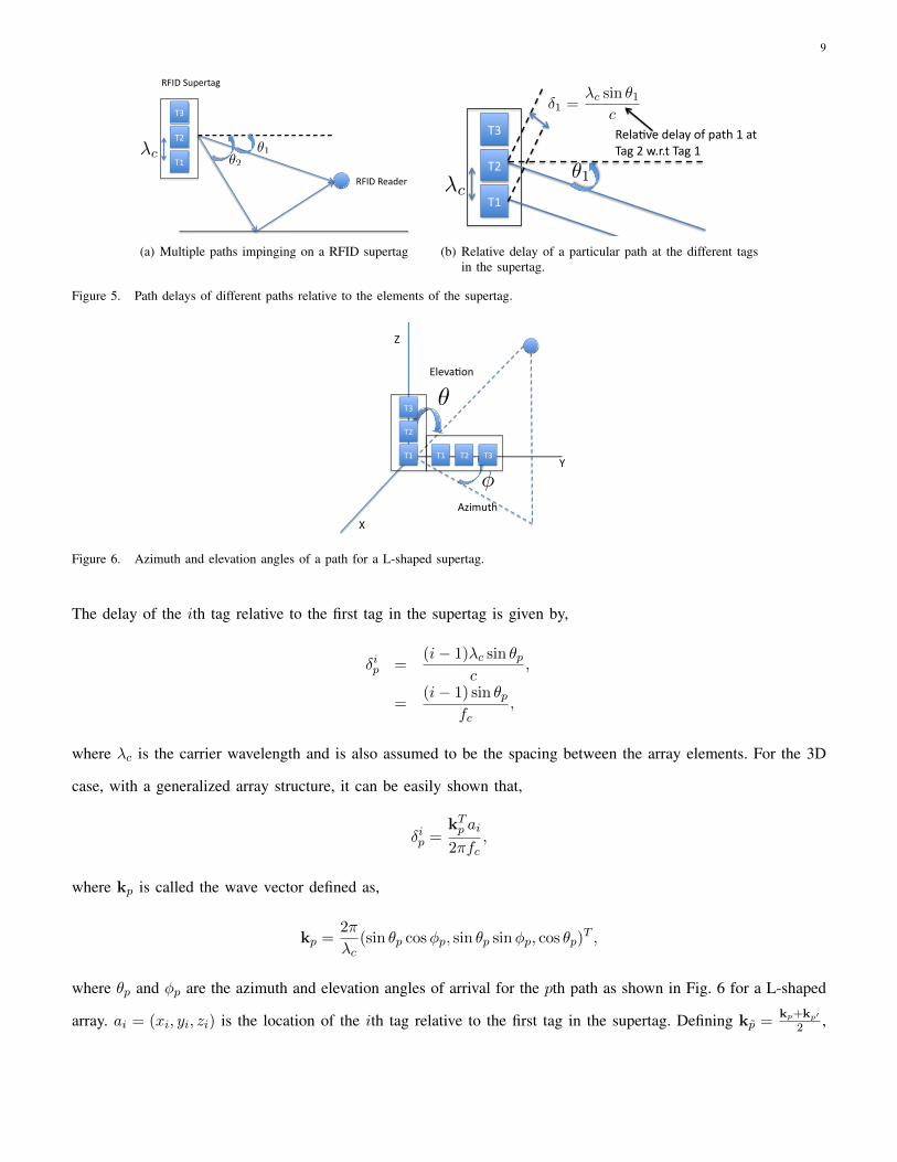
additional delay of δjp at the jth tag relative to the first tag. Fig. 5 depicts this for a linear array of tags in 2D. In

all our simulations, we model the path gains as Rayleigh fading random variables.

The signals from multiple paths arriving at different angles superimpose at each tag in the supertag. Each tag

backscatters the impinged signal after modulating it with its own unique CDMA sequence. Further, we assume

7

that all the tags in the supertag modulate the signal with a common sequence that serves as the unique ID for that

supertag. This makes it easier to distinguish different supertags. We assume symmetrical forward and backward

channels from the reader to the supertag. Thus each modulated signal from a particular tag in the array undergoes

a relative delay with respective to the first tag in the array and further goes through all the different paths before

impinging on the receiver antenna at the reader.

The received signal is demodulated and projected onto each of the individual CDMA sequences of the different

tags in the supertag to retrieve the signals from different elements of the supertag. The azimuth and elevation

angles (see Fig. 6) of the different paths are recovered using an array processing algorithm like MUltiple SIgnal

Classification (MUSIC) [19]. Amongst the pairs of azimuth and elevation angles that are obtained, the ambiguity

as to which of these pairs correspond to the actual LOS path remains. Further, none of the angles could correspond

to the LOS path if the gain of the LOS path were to be small relative to the other paths. We now express the

received signal in terms of the elevation and azimuth angles and the different system parameters and explain how

MUSIC can be used to obtain estimates of the path angles.

Let Tc be the chip width of the CDMA sequence. Let s(t) be the bandlimited modulation signal with a main

lobe width of Tc. For example, s(t) could be a square wave of width Tc or a raised cosine pulse. We use a raised

cosine pulse in all our simulations. If {cin}N−1n=0 is the N length CDMA sequence associated with the ith tag and

{rk}K−1k=0 is the K length ID of the supertag, then the modulation signal at the ith tag has the following structure,

K−1∑

k=0

rk

N−1∑

n=0

cins(t− nTc − kTs),

where Ts is the symbol width of the supertag ID. It is assumed that Ts > NTc. The ith tag modulates the carrier

signal with the above CDMA sequence. The carrier signal is received at the supertag after reflection from multiple

paths. Let gp be the gain of the pth path, ∆p the delay and δip the relative delay of the pth path at the ith tag

relative to the first tag in the supertag. The signal after modulation from the ith tag is given by,

P∑

p=1

gp

K−1∑

k=0

rk

N−1∑

n=0

cins(t− nTc − kTs −∆p − δip).

Here we use the same notation s(.) to denote the baseband as well as the passband signal and do not explicitly

show the carrier signal for ease of notation. This signal traverses the reverse channel and is received at the receiver.

8

The superimposed signal at the receiver from all the tags in the array is given by,

L∑

i=1

P∑

p′=1

gp′P∑

p=1

gp

K−1∑

k=0

rk

N−1∑

n=0

cins(t− nTc − kTs

−∆p − δip −∆p′ − δip′),

where L is the number of tags in the array. Assume that the gain introduced by each of the tags in the supertag is

the same and is normalized to unity. Let fc be the carrier frequency. The signal after demodulation and low pass

filtering at the receiver is given by,

r(t) =

L∑

i=1

P∑

p′=1

gp′P∑

p=1

gpe−j2πfc(δip+δi

p′+∆p+∆p′ )

K−1∑

k=0

rk

N−1∑

n=0

cins(t− nTc − kTs) + n(t),

where n(t) is the thermal noise process at the receiver, which we can model as N (0, σ2). The delays ∆p and ∆p′

do not depend on the index i, since they are common to all the elements of the supertag. Hence the phase term

e−j2πfc(∆p+∆p′ ) can be included in the path gain terms gp and gp′ , to get the simplified expression,

r(t) =

L∑

i=1

P∑

p′=1

gp′P∑

p=1

gpe−j2πfc(δip+δi

p′ )

K−1∑

k=0

rk

N−1∑

n=0

cins(t− nTc − kTs) + n(t),

where we use the same notations gp and gp′ to represent the modified path gains for ease of notation.

The received signal is projected onto each of the individual CDMA sequences of the tags to extract the signal,

ri(k), corresponding to each element of the supertag as follows,

ri(k) =

∫ kTs

(k−1)Ts

r(t)

N−1∑

n=0

cins(t− nTc − kTs)dt,

=

N−1∑

n=0

cin

∫ kTs

(k−1)Ts

r(t)s(t− nTc − kTs)dt,

≈P∑

p=1

P∑

p′=1

gpgp′e−j2πfc(δip+δi

p′ )rk + ni(k).

Let us now evaluate the relative delays δip. Consider a 2D case with a linear antenna array as shown in Fig. 5.

9

!"#

!$#

!%#

&'()#&*+,*-#

&'()#./0*-1+2#

θ1θ2

λc

(a) Multiple paths impinging on a RFID supertag

!"#

!$#

!%#

θ1

δ1 =λc sin θ1

c&'()*+'#,'()-#./#0)12#%#)1##!)3#$#45651#!)3#%##

λc

(b) Relative delay of a particular path at the different tagsin the supertag.

Figure 5. Path delays of different paths relative to the elements of the supertag.

!"#

!$#

!%# !"#!$#!%#

θ

φ>#

?#

@#

A6*5+BC3#

:D4E/1F#

Figure 6. Azimuth and elevation angles of a path for a L-shaped supertag.

The delay of the ith tag relative to the first tag in the supertag is given by,

δip =(i− 1)λc sin θp

c,

=(i− 1) sin θp

fc,

where λc is the carrier wavelength and is also assumed to be the spacing between the array elements. For the 3D

case, with a generalized array structure, it can be easily shown that,

δip =kTp ai

2πfc,

where kp is called the wave vector defined as,

kp =2π

λc(sin θp cosφp, sin θp sinφp, cos θp)

T ,

where θp and φp are the azimuth and elevation angles of arrival for the pth path as shown in Fig. 6 for a L-shaped

array. ai = (xi, yi, zi) is the location of the ith tag relative to the first tag in the supertag. Defining kp =kp+kp′

2 ,

10

we can rewrite the extracted signal at the receiver as follows,

ri(k) =

P 2∑

p=1

gprke−j2kT

p ai ,

where the first P terms in the above summation correspond to the P paths and the rest of the terms are combinations

of the different paths. Note that all the paths p are clearly not independent since many of these are combinations

of the others. However, in our estimation, we will treat these as separate paths for simplicity. Further, in practice,

given the low gains of many of these paths, only the significant paths with large gains will stand out and the rest

of the cross terms would be small.

The above system of equations can be written as,

r(k) = Bx(k) + n(k),

where the matrix B, known as the array response matrix, is given by,

B =

e−j2k1T a1 e−j2k2

T a1 ... e−j2kP2T a1

... ... ... ...

e−j2k1T aL e−j2k2

T aL ... e−j2kP2T aL

,

= [b(θ1, φ1)....b(θP 2 , φP 2)] ,

and x(k) is given by,

x(k) =

g21 rk

g22 rk

...

g2P rk

...

gP−1gP rk

.

At this juncture, the goal is to obtain estimates of the azimuth and elevation angles, {θp, φp}Pp=1, of the different

paths. There are many array processing algorithms [19] such as MUSIC, ESPRIT etc., that can be used here.

Algorithms like ESPRIT require a Vandermonde-like matrix structure for B. However, if we are interested in a

general tag array structure, this does not hold. Hence we will use MUSIC for now and one can always replace this

with a better estimator if available.

11

0

50

100

0

50

1000

0.5

1

1.5

2

azhimuth ( )

MUSIC Spectrum

elevation ( )

Figure 7. Example of a MUSIC spectrum

The Vandermonde-like matrix B has rank P 2 with high probability assuming that the NLOS path angles are

uniform randomly picked. Assuming the additive noise to be Gaussian with variance σ2, the covariance matrix of

the received signal S ∈ RN×N is given by,

S = E[r(k)r(k)H ]

= BSXBH + σ2I.

Note that the rank of BSXBH is P 2 assuming SX to be full rank. Given an eigen decomposition of S, the N −P 2

eigen vectors corresponding to the eigen value σ2 lie in the null space of BSXBH and thereby in the null space

of BH . Thus, given an estimate of the covariance matrix S, the path angles can be estimated as the P 2 highest

peaks of,1

bH(θ, φ)QHNQNb(θ, φ),

where QN is the matrix of eigen vectors corresponding to the noise signal space of S. Fig. 7 shows the MUSIC

spectrum as a function of the azimuth and elevation angles. The peaks correspond to the arrival angles of the

different paths. Note that here we assumed L > P 2. However, in practice it might be expensive to have a large L.

Here we will be able to resolve at most L paths since the rank of A would be L. In practice, given that some of

the paths have low gains, the number of terms would be small since the gains are reinforced/attenuated due to the

signals traversing the different paths in the forward and backward directions. Further, these uncertainties can be

captured in the parameters of the statistical model that we build later and all we need for the system to function

is that some fraction of the measurements are LOS. These issues can be tackled by exploiting the redundancy in

measurements obtained from deploying many supertags in the environment.

12

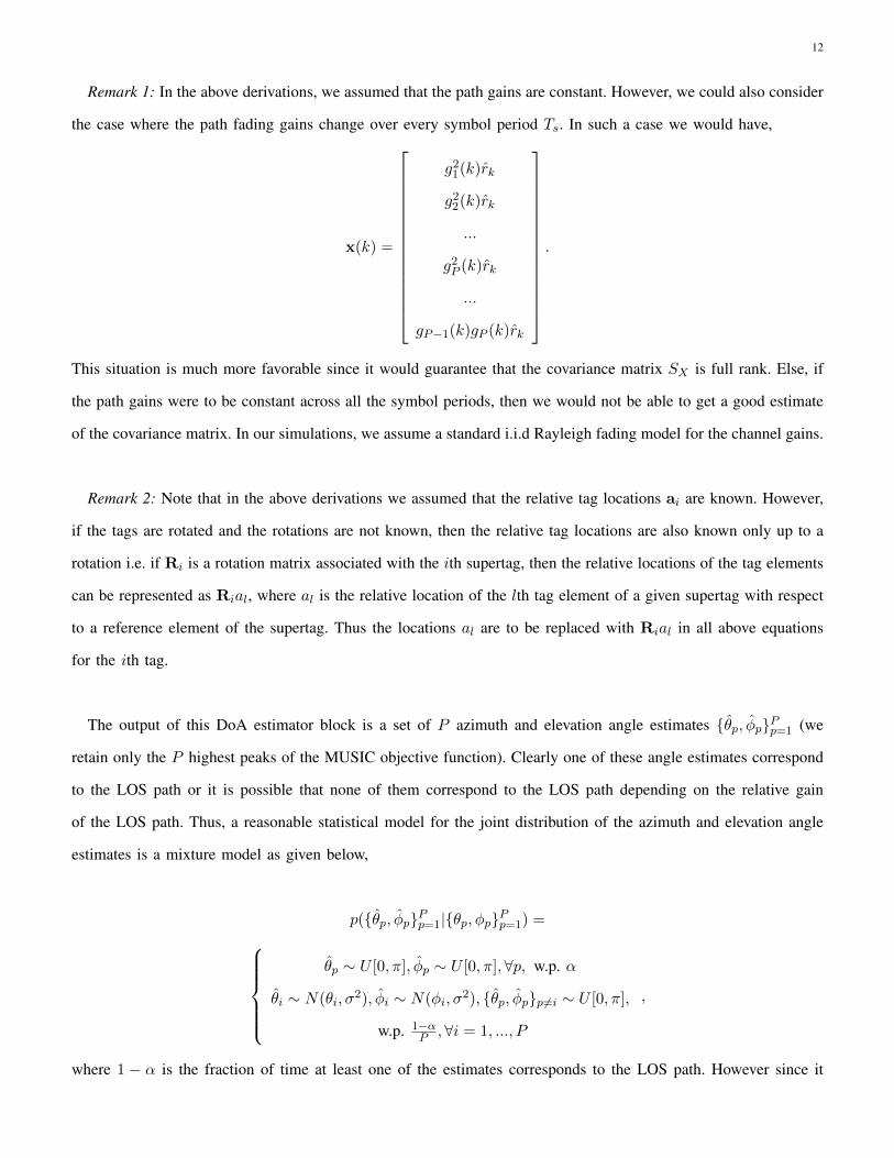
Remark 1: In the above derivations, we assumed that the path gains are constant. However, we could also consider

the case where the path fading gains change over every symbol period Ts. In such a case we would have,

x(k) =

g21(k)rk

g22(k)rk

...

g2P (k)rk

...

gP−1(k)gP (k)rk

.

This situation is much more favorable since it would guarantee that the covariance matrix SX is full rank. Else, if

the path gains were to be constant across all the symbol periods, then we would not be able to get a good estimate

of the covariance matrix. In our simulations, we assume a standard i.i.d Rayleigh fading model for the channel gains.

Remark 2: Note that in the above derivations we assumed that the relative tag locations ai are known. However,

if the tags are rotated and the rotations are not known, then the relative tag locations are also known only up to a

rotation i.e. if Ri is a rotation matrix associated with the ith supertag, then the relative locations of the tag elements

can be represented as Rial, where al is the relative location of the lth tag element of a given supertag with respect

to a reference element of the supertag. Thus the locations al are to be replaced with Rial in all above equations

for the ith tag.

The output of this DoA estimator block is a set of P azimuth and elevation angle estimates {θp, φp}Pp=1 (we

retain only the P highest peaks of the MUSIC objective function). Clearly one of these angle estimates correspond

to the LOS path or it is possible that none of them correspond to the LOS path depending on the relative gain

of the LOS path. Thus, a reasonable statistical model for the joint distribution of the azimuth and elevation angle

estimates is a mixture model as given below,

p({θp, φp}Pp=1|{θp, φp}Pp=1) =

θp ∼ U [0, π], φp ∼ U [0, π],∀p, w.p. α

θi ∼ N(θi, σ2), φi ∼ N(φi, σ

2), {θp, φp}p 6=i ∼ U [0, π],

w.p. 1−αP ,∀i = 1, ..., P

,

where 1 − α is the fraction of time at least one of the estimates corresponds to the LOS path. However since it

13

0 0.5 1 1.5 2 2.5 3 3.5 40

0.1

0.2

0.3

0.4

0.5

0.6

0.7

0.8

0.9

1

Gain of the line of sight path

Frac

tion

of li

neof

sigh

t mea

sure

men

ts (1

)

Fraction of LOS measurements as a function of the gain of the LOS path

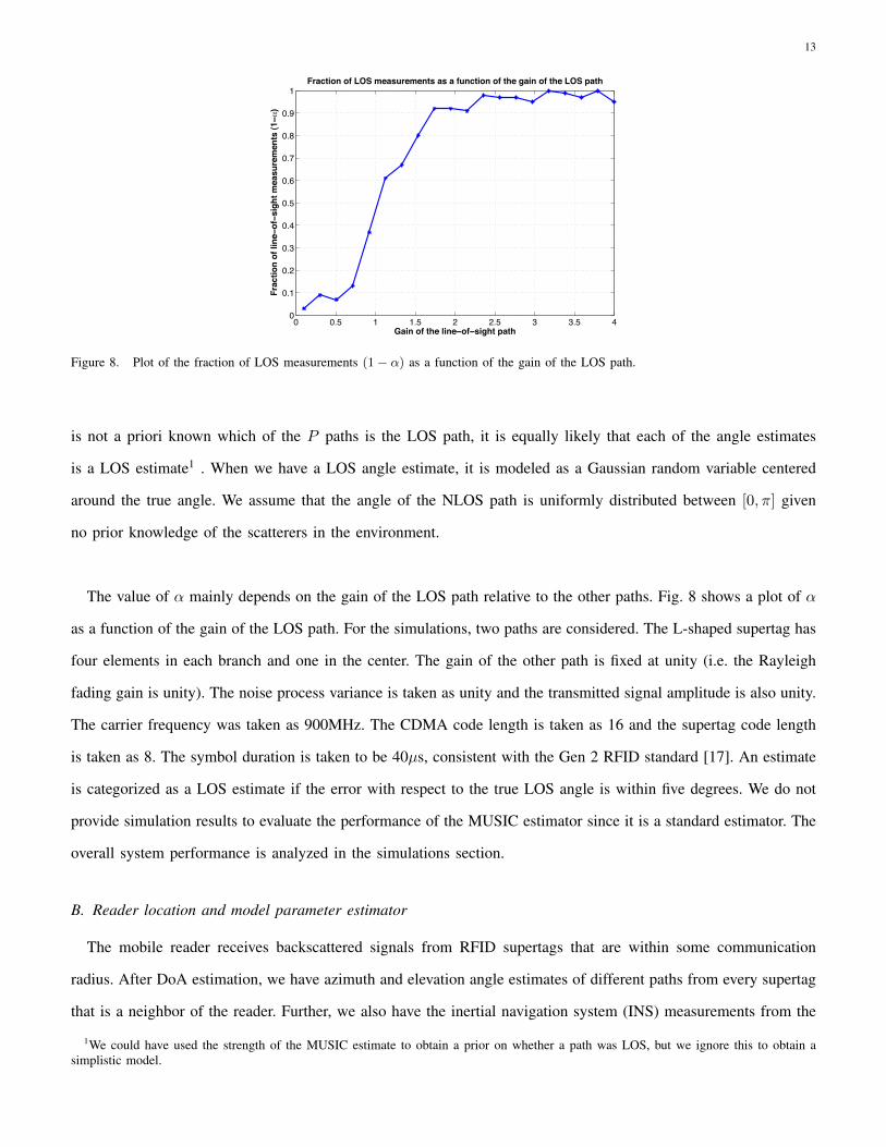
Figure 8. Plot of the fraction of LOS measurements (1− α) as a function of the gain of the LOS path.

is not a priori known which of the P paths is the LOS path, it is equally likely that each of the angle estimates

is a LOS estimate1 . When we have a LOS angle estimate, it is modeled as a Gaussian random variable centered

around the true angle. We assume that the angle of the NLOS path is uniformly distributed between [0, π] given

no prior knowledge of the scatterers in the environment.

The value of α mainly depends on the gain of the LOS path relative to the other paths. Fig. 8 shows a plot of α

as a function of the gain of the LOS path. For the simulations, two paths are considered. The L-shaped supertag has

four elements in each branch and one in the center. The gain of the other path is fixed at unity (i.e. the Rayleigh

fading gain is unity). The noise process variance is taken as unity and the transmitted signal amplitude is also unity.

The carrier frequency was taken as 900MHz. The CDMA code length is taken as 16 and the supertag code length

is taken as 8. The symbol duration is taken to be 40µs, consistent with the Gen 2 RFID standard [17]. An estimate

is categorized as a LOS estimate if the error with respect to the true LOS angle is within five degrees. We do not

provide simulation results to evaluate the performance of the MUSIC estimator since it is a standard estimator. The

overall system performance is analyzed in the simulations section.

B. Reader location and model parameter estimator

The mobile reader receives backscattered signals from RFID supertags that are within some communication

radius. After DoA estimation, we have azimuth and elevation angle estimates of different paths from every supertag

that is a neighbor of the reader. Further, we also have the inertial navigation system (INS) measurements from the

1We could have used the strength of the MUSIC estimate to obtain a prior on whether a path was LOS, but we ignore this to obtain asimplistic model.

14

u(t − 1) u(t) u(t + 1)

(a3,R3)

(a6, R6)

(a2, R2)(a1,R1)

(a4,R4) (a5,R5) (a7,R7)

!"#$"%&'()#*(+&

,#'-.%#/"$&012"%/#3& 4+)#'-.%#/"$&012"%/#3&

�θ4p(t − 1)φ5p(t − 1)

�

�θ1p(t − 1)φ1p(t − 1)

�

�θ5p(t − 1)φ5p(t − 1)

�

�θ2p(t)φ2p(t)

�

�θ5p(t)φ5p(t)

� �θ6p(t)φ6p(t)

�

�θ2p(t + 1)φ2p(t + 1)

��θ3p(t + 1)φ3p(t + 1)

�

�θ6p(t + 1)φ6p(t + 1)

� �θ7p(t + 1)φ7p(t + 1)

�

5+3'"&"6*7#/"6&

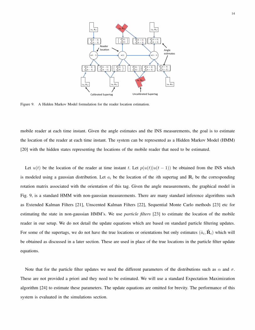
Figure 9. A Hidden Markov Model formulation for the reader location estimation.

mobile reader at each time instant. Given the angle estimates and the INS measurements, the goal is to estimate

the location of the reader at each time instant. The system can be represented as a Hidden Markov Model (HMM)

[20] with the hidden states representing the locations of the mobile reader that need to be estimated.

Let u(t) be the location of the reader at time instant t. Let p(u(t)|u(t − 1)) be obtained from the INS which

is modeled using a gaussian distribution. Let ai be the location of the ith supertag and Ri be the corresponding

rotation matrix associated with the orientation of this tag. Given the angle measurements, the graphical model in

Fig. 9, is a standard HMM with non-gaussian measurements. There are many standard inference algorithms such

as Extended Kalman Filters [21], Unscented Kalman Filters [22], Sequential Monte Carlo methods [23] etc for

estimating the state in non-gaussian HMM’s. We use particle filters [23] to estimate the location of the mobile

reader in our setup. We do not detail the update equations which are based on standard particle filtering updates.

For some of the supertags, we do not have the true locations or orientations but only estimates (ai, Ri) which will

be obtained as discussed in a later section. These are used in place of the true locations in the particle filter update

equations.

Note that for the particle filter updates we need the different parameters of the distributions such as α and σ.

These are not provided a priori and they need to be estimated. We will use a standard Expectation Maximization

algorithm [24] to estimate these parameters. The update equations are omitted for brevity. The performance of this

system is evaluated in the simulations section.

15

u1

u2

u3

k3

(a,R)k1

k2

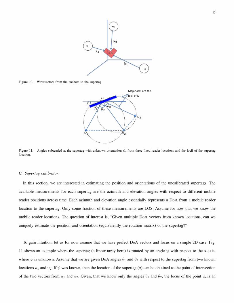
Figure 10. Wavevectors from the anchors to the supertag

ψ

θ1 θ2

u1 u2

a

u3

θ3

!"#$%&"%'(&"%)&*+)&&

,$'--&$.&!"

Figure 11. Angles subtended at the supertag with unknown orientation ψ, from three fixed reader locations and the locii of the supertaglocation.

C. Supertag calibrator

In this section, we are interested in estimating the position and orientations of the uncalibrated supertags. The

available measurements for each supertag are the azimuth and elevation angles with respect to different mobile

reader positions across time. Each azimuth and elevation angle essentially represents a DoA from a mobile reader

location to the supertag. Only some fraction of these measurements are LOS. Assume for now that we know the

mobile reader locations. The question of interest is, “Given multiple DoA vectors from known locations, can we

uniquely estimate the position and orientation (equivalently the rotation matrix) of the supertag?”

To gain intuition, let us for now assume that we have perfect DoA vectors and focus on a simple 2D case. Fig.

11 shows an example where the supertag (a linear array here) is rotated by an angle ψ with respect to the x-axis,

where ψ is unknown. Assume that we are given DoA angles θ1 and θ2 with respect to the supertag from two known

locations u1 and u2. If ψ was known, then the location of the supertag (a) can be obtained as the point of intersection

of the two vectors from u1 and u2. Given, that we know only the angles θ1 and θ2, the locus of the point a, is an

16

arc of the circle defined by the chord (u1−u2) and the included angle θ2−θ1. Thus, if we had another location u3

and the corresponding angle-of-arrival, we could obtain the location of the supertag a, as the intersection of these

two circles as shown in Fig. 11. Once the location of the supertag is estimated, it is easy to estimate its orientation ψ.

Similarly, in the 3D case, we have estimates of the azimuth and elevation angles relative to the rotated supertag.

Each azimuth and elevation angle estimate is equivalent to having an estimate of the unit vector originating from the

fixed reader location in the direction of the rotated supertag. This is essentially a scaled version of the wavevector

(see Fig. 10). We will use the same terminology “wavevector” and the notation to refer to this unit vector. Let ki

be the wavevector from the ith anchor to the supertag. In the case when the orientation of the supertag is known

and the wavevectors are known exactly, the location of the supertag is obtained as the point of intersection of any

two wavevectors. Now consider the case when the rotation of the supertag is unknown. The array response matrix

B would have terms of the form kTi (Raj) where R is the rotation matrix that rotates the supertag array. The terms

can be equivalently written as (RTki)Taj . Hence the DoA estimator provides us with the estimates of the rotated

wavevectors ki = RTki. Note that all the wavevectors undergo the same rotation. Thus the problem of interest is

the joint estimation of the rotation matrix and the supertag location given these rotated wavevectors.

Using the intuition from the 2D case, we can calculate the angle between two such vectors as cos θij = kTi kj =

kTi kj , which is independent of the rotation matrix. The locus of the supertag location given the reader locations

ui and uj and the included angle θij , is a spindle torus [25] (if the angle is π/2, then it is a sphere). Given four

such vectors, the location of the supertag can be obtained as the intersection of the corresponding different spindle

tori. Once the location of the supertag is obtained, the rotation matrix can be estimated using estimates of the true

and the rotated wavevectors. We will now see how to estimate the location and orientation of the supertag given

M DoA vectors, k1, ...., kM , from known reader locations u1, ..., uM . We have the following,

kTi kj = kTi kj ,

(ui − a)T (uj − a)

||ui − a||||uj − a||= kTi kj ,

(ui − a)T (uj − a) = ||ui − a||||uj − a||kTi kj .

Thus, given noisy estimates of the rotated wavevectors {ki}, the estimate of the supertag location can be obtained

as a solution of the following least squares optimization problem,

17

a = arg mina

∑

i,j

((ui − a)T (uj − a)− ||ui − a||||uj − a||kTi kj)

2.

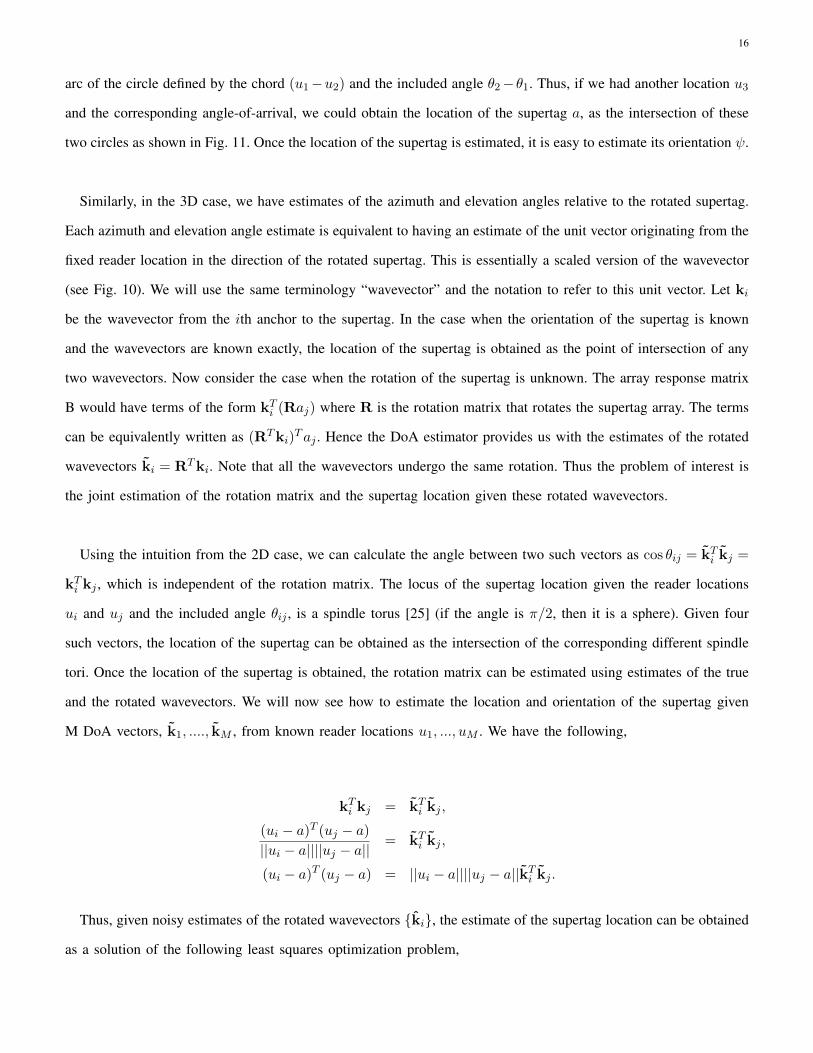
The above optimization problem is highly non-convex in the general case and hence a simple gradient descent

algorithm would not yield a good solution unless the initial point is carefully chosen. However, we have observed

that the objective function has nice convexity properties whenever the supertag location is within the convex hull of

the fixed reader locations. In the 2D case, it might be reasonable to assume that the supertag lies within the convex

hull of the reader locations. However, in 3D, this might not be a valid assumption for many interesting application

scenarios. For example, in the case of indoor localization, typically the supertags will be deployed on the walls of

the indoor environment (see Fig. 1). Even in this case, we can observe some interesting convexity properties. For

example, consider the supertags present on the floor. Suppose we fix the z-coordinate of the supertag location and

evaluate the objective function only as a function of the x and y coordinates. In this case, we have observed that,

when the z-coordinate is taken as the true z-coordinate of the supertag, then the objective function is convex as

long as the reader locations are well spread out. In particular, the x and y coordinates of the supertag should be in

the convex hull of the x and y coordinates of the reader locations. Fig. 12 shows a plot of the objective function

as a function of the x and y coordinates. Thus a natural solution to solving the above optimization problem is to

sweep through all possible z-coordinates and obtain the minimum for each z value by using a gradient descent

on the optimization. The minimum value over all possible z would give us the global minimum of the objective

function. Of course, in the case when we know the z-coordinate exactly as in the above example, we can just solve

the optimization problem as a function of x and y using a simple gradient descent since the objective function is

convex. Similarly one can use the same argument to estimate supertag locations on the side walls by fixing the

corresponding x or the y coordinates.

Given a location estimate a for the supertag, its rotation can be estimated as follows. We have that,

R[k1...kM ] = [k1...kM ],

R[k1...kM ] =

[(u1 − a)

||u1 − a||...

(uM − a)

||uM − a||

],

R = arg minR R[k1...kM ]−[

(u1 − a)

||u1 − a||...

(uM − a)

||uM − a||

].

The above problem is a simple least squares problem and R can be estimated using the pseudo-inverse. In order

18

0

5

10

0

5

100

0.5

1

1.5

2

2.5x 104

X coordinate

Objective function as a function of the X and Y coordinate

Y coordinate

Obj

ectiv

e fu

nctio

n va

lue

Figure 12. Convexity of the objective function for a fixed z-coordinate.

location estimate is picked as the one with the minimumobjective function value.

The number of iterations, J , of the RANSAC al-gorithm can be calculated as follows. Let p be theprobability that we do not encounter a LOS set evenonce in J trials. We want this probability to be δ. Weare given that (1−α) is the probability that a reading isLOS. Assume that M >> K. We have the following,

p = (1 − (1 − α)K)J ,

(1 − (1 − α)K)J = δ,

J =log δ

log(1 − (1 − α)K).

Now, we do not have the true mobile reader locationsand we will use the estimated locations in our calibrationalgorithm. Algorithm 1 details the supertag calibrationprocess.

Algorithm 1 Supertag calibration1: Input: NLOS fraction α, Reader location estimates {u1, ...., uM},

Rotated wavevector estimates {k1, ....., kM}.2: Choose K ≥ 4, J = log δ

log(1−(1−α)K).

3: for i = 1 to J do4: Sample K wavevectors randomly, {ki1 , ....., kiK

}.5:

ai = arg min�

i,j∈S((ui−a)T (uj−a)−||ui−a||||uj−a||kT

i kj)2,

where S is the set of indices of the sampled set. Solve this optimizationproblem using the modified ML algorithm.

6: If the objective function value is the minimum of all the iterations sofar, then a = ai. R is obtained using the least squares optimizationfollowed by SVD normalization.

7: end for8: Output: Supertag location and orientation estimates a, R.

Fig. 12 and 13 show plots of the error in localizationand orientation as a function of the fraction of NLOSmeasurements. The simulations were carried out byhaving random supertag locations in a 3 × 3 × 10box and fixed reader locations randomly placed in a4 × 4 × 4 box. Thus the z-coordinate of the supertagcan be large which essentially keeps the tag outsidethe convex hull of the reader locations. However, for afixed z-coordinate, the optimization problem is convex.The modified gradient descent runs by sweeping acrossthe z−coordinates and minimizing over the other twocoordinates. The number of readers were taken to be100, which is reasonable if we assume that we have

0.1 0.2 0.3 0.4 0.5 0.6 0.7 0.8 0.9 10

0.5

1

1.5

2

2.5

3

3.5

4

4.5

Fraction of NLOS measurements ( )

Erro

r in

the

tag

loca

tion

estim

ate

(m)

Error in the tag location estimate as a function of

Figure 12. Plot of the absolute error in tag location estimates as afunction of α.

0.1 0.2 0.3 0.4 0.5 0.6 0.7 0.8 0.9 10

0.5

1

1.5

2

2.5

Fraction of NLOS measurements ( )

Erro

r in

estim

atin

g th

e ro

tatio

n m

atrix

Error in estimating the rotation matrix as a function of

Figure 13. Plot of the estimation error in orientations as a functionof α.

0.1 0.2 0.3 0.4 0.5 0.6 0.7 0.80

2000

4000

6000

8000

10000

12000

Fraction of NLOS measurements ( )

Num

ber o

f ite

ratio

ns n

eede

d fo

r rel

iabl

e es

timat

ion

with

hig

h pr

obab

ility

(99%

)

Computational complexity as a function of

Figure 14. Plot of the number of iterations needed for the RANSACalgorithm as a function of α.

rotation can be estimated as follows. We have that,

R[k1...kM ] = [k1...kM ],

R[k1...kM ] =

�(u1 − a)

||u1 − a|| ...(uM − a)

||uM − a||

�,

R = arg minR R[k1...kM ]−�

(u1 − a)

||u1 − a|| ...(uM − a)

||uM − a||

�.

The above problem is a simple least squares problemand R can be estimated using the pseudo-inverse. Inorder to have R as a valid rotation matrix, we take thesingular value decomposition of the estimated matrixand set the singular values to unity.

So far, we assumed that the available DoA vectorsare the true LOS vectors. However, in the originalapplication, we have a fraction of these to be NLOS.The simple least squares formulation is not robust toNLOS and it can lead to very large estimation errors.In order to tackle NLOS measurements, we proposeto use a Random Sample Consensus (RANSAC)algorithm [26]. We are given that (1 − α) fractionof the measurements are LOS. In order to obtain anunambiguous location estimate of the supertag, we needat least four DoA vectors. The underlying principle ofthe RANSAC algorithm is to randomly choose subsetsof K ≥ 4 DoA vectors and compute the least squaresestimate. The process is repeated multiple times so thatwe encounter a LOS set of K measurements at leastonce with high probability. The location estimate ispicked as the one with the minimum objective functionvalue.

The number of iterations, J , of the RANSAC al-

gorithm can be calculated as follows. Let p be theprobability that we do not encounter a LOS set evenonce in J trials. We want this probability to be δ. Weare given that (1 − α) fraction of the measurements areLOS. Assume that M >> K. We have the following,

p = (1 − (1 − α)K)J ,

(1 − (1 − α)K)J = δ,

J =log δ

log(1 − (1 − α)K).

In our system, we use the estimated locations of themobile readers in place of the true locations. Algorithm1 details the supertag calibration process.

Algorithm 1 Supertag calibration1: Input: NLOS fraction α, Reader location estimates {u1, ...., uM},

Rotated wavevector estimates {k1, ....., kM}.2: Choose K ≥ 4, J = log δ

log(1−(1−α)K).

3: for i = 1 to J do4: Sample K wavevectors randomly, {ki1 , ....., kiK

}.5:

ai = arg min�

l,m∈S((ul−a)T (um−a)−||ul−a||||um−a||kT

l km)2,

Ri = arg min�

l∈S

��������Rkl −

(ul − ai)

||ul − ai||

�������� ,

where S is the set of indices of the sampled set. Solve this optimizationproblem using the modified ML algorithm.

6: If the objective function value is the minimum of all the iterations sofar, then a = ai. R = UV T where Ri = UΣV T .

7: end for8: Output: Supertag location and orientation estimates a, R.

The simulations were carried out for random supertaglocations in a 3 × 3 × 10 box and fixed readerlocations randomly placed in a 4 × 4 × 4 box. Thusthe z-coordinate of the supertag can be large whichessentially keeps the tag outside the convex hull of thereader locations. However, for a fixed z-coordinate, wehave observed that the optimization problem is convex.The modified gradient descent runs by sweeping acrossthe z−coordinates and minimizing over the other twocoordinates. The number of readers were taken to be100, which is reasonable if we assume that we havemany readers navigating the environment across time,thus providing readings both across time and space.K was fixed at 5. The other parameters are similarto what we used to analyze the performance of theDoA estimator. The reader locations were slightlyperturbed and the true values were not used. The yaw,pitch and roll angles for the supertags were taken

So far, we assumed that the available DoA vectorsare the true LOS vectors. However, in the originalapplication, we have a fraction of these to be NLOS.The simple least squares formulation is not robust toNLOS and it can lead to very large estimation errors.In order to tackle NLOS measurements, we proposeto use a Random Sample Consensus (RANSAC)algorithm [26]. We are given that (1 − α) fractionof the measurements are LOS. In order to obtain anunambiguous location estimate of the supertag, we needat least four DoA vectors. The underlying principle ofthe RANSAC algorithm is to randomly choose subsetsof K ≥ 4 DoA vectors and compute the least squaresestimate. The process is repeated multiple times so thatwe encounter a LOS set of K measurements at leastonce with high probability. The location estimate ispicked as the one with the minimum objective functionvalue.

The number of iterations, J , of the RANSAC al-gorithm can be calculated as follows. Let p be theprobability that we do not encounter a LOS set evenonce in J trials. We want this probability to be δ. Weare given that (1 − α) fraction of the measurements areLOS. Assume that M >> K. We have the following,

p = (1 − (1 − α)K)J ,

(1 − (1 − α)K)J = δ,

J =log δ

log(1 − (1 − α)K).

In our system, we use the estimated locations of themobile readers in place of the true locations. Algorithm

0.1 0.2 0.3 0.4 0.5 0.6 0.7 0.8 0.9 10

0.5

1

1.5

2

2.5

3

3.5

4

4.5

Fraction of NLOS measurements ( )

Erro

r in

the

tag

loca

tion

estim

ate

(m)

Error in the tag location estimate as a function of

Figure 13. Plot of the absolute error in tag location estimates as afunction of α.

1 details the supertag calibration process.

Algorithm 1 Supertag calibration1: Input: NLOS fraction α, Reader location estimates {u1, ...., uM},

Rotated wavevector estimates {k1, ....., kM}.2: Choose K ≥ 4, J = log δ

log(1−(1−α)K).

3: for i = 1 to J do4: Sample K wavevectors randomly, {ki1 , ....., kiK

}.5:

ai = arg min�

l,m∈S((ul−a)T (um−a)−||ul−a||||um−a||kT

l km)2,

Ri = arg min�

l∈S

��������Rkl −

(ul − ai)

||ul − ai||

�������� ,

where S is the set of indices of the sampled set. Solve this optimizationproblem using the modified gradient descent algorithm.

6: If the objective function value is the minimum of all the iterations sofar, then a = ai. R = UV T where Ri = UΣV T .

7: end for8: Output: Supertag location and orientation estimates a, R.

The simulations were carried out for random supertaglocations in a 3× 3× 10 box and fixed reader locationsrandomly placed in a 4 × 4 × 4 box. Thus the z-coordinate of the supertag can be large and unknownwhich essentially keeps the tag outside the convexhull of the reader locations. However, for a fixedz-coordinate, we have observed that the optimizationproblem is convex. The modified gradient descent runsby sweeping across the z−coordinates and minimizingover the other two coordinates. The number of readerswas taken to be 100, which is reasonable assuming

to have R as a valid rotation matrix, we take the singular value decomposition of the estimated matrix and set the

singular values to unity.

So far, we assumed that the available DoA vectors are the true LOS vectors. However, in the original application,

we have a fraction of these to be NLOS. The simple least squares formulation is not robust to NLOS and it can

lead to very large estimation errors. In order to tackle NLOS measurements, we propose to use a Random Sample

Consensus (RANSAC) algorithm [26]. We are given that (1− α) fraction of the measurements are LOS. In order

to obtain an unambiguous location estimate of the supertag, we need at least four DoA vectors. The underlying

principle of the RANSAC algorithm is to randomly choose subsets of K ≥ 4 DoA vectors and compute the least

squares estimate. The process is repeated multiple times so that we encounter a LOS set of K measurements at

least once with high probability. The location estimate is picked as the one with the minimum objective function

value.

19

0.1 0.2 0.3 0.4 0.5 0.6 0.7 0.8 0.9 10

0.5

1

1.5

2

2.5

3

3.5

4

4.5

Fraction of NLOS measurements ( )

Erro

r in

the

tag

loca

tion

estim

ate

(m)

Error in the tag location estimate as a function of

Figure 13. Plot of the absolute error in tag location estimates as a function of α.

0.1 0.2 0.3 0.4 0.5 0.6 0.7 0.8 0.9 10

0.5

1

1.5

2

2.5

Fraction of NLOS measurements ( )

Erro

r in

estim

atin

g th

e ro

tatio

n m

atrix

Error in estimating the rotation matrix as a function of

Figure 14. Plot of the estimation error in orientations as a function of α.

The number of iterations, J , of the RANSAC algorithm can be calculated as follows. Let p be the probability

that we do not encounter a LOS set even once in J trials. We want this probability to be δ. We are given that

(1− α) fraction of the measurements are LOS. Assume that M >> K. We have the following,

p = (1− (1− α)K)J ,

(1− (1− α)K)J = δ,

J =log δ

log(1− (1− α)K).

In our system, we use the estimated locations of the mobile readers in place of the true locations. Algorithm 1

details the supertag calibration process.

20

0.1 0.2 0.3 0.4 0.5 0.6 0.7 0.80

2000

4000

6000

8000

10000

12000

Fraction of NLOS measurements ( )

Num

ber o

f ite

ratio

ns n

eede

d fo

r rel

iabl

e es

timat

ion

with

hig

h pr

obab

ility

(99%

)

Computational complexity as a function of

Figure 15. Plot of the number of iterations needed for the RANSAC algorithm as a function of α.

The simulations were carried out for random supertag locations in a 3× 3× 10 box and fixed reader locations

randomly placed in a 4×4×4 box. Thus the z-coordinate of the supertag can be large and unknown which essentially

keeps the tag outside the convex hull of the reader locations. However, for a fixed z-coordinate, we have observed

that the optimization problem is convex. The modified gradient descent runs by sweeping across the z−coordinates

and minimizing over the other two coordinates. The number of readers was taken to be 100, which is reasonable

assuming that we have many readers navigating the environment across time, thus providing readings both across

time and space. K was fixed at 5. The other parameters are similar to what we used in analyzing the performance of

the DoA estimator. The reader locations were slightly perturbed and the true values were not used. The yaw, pitch

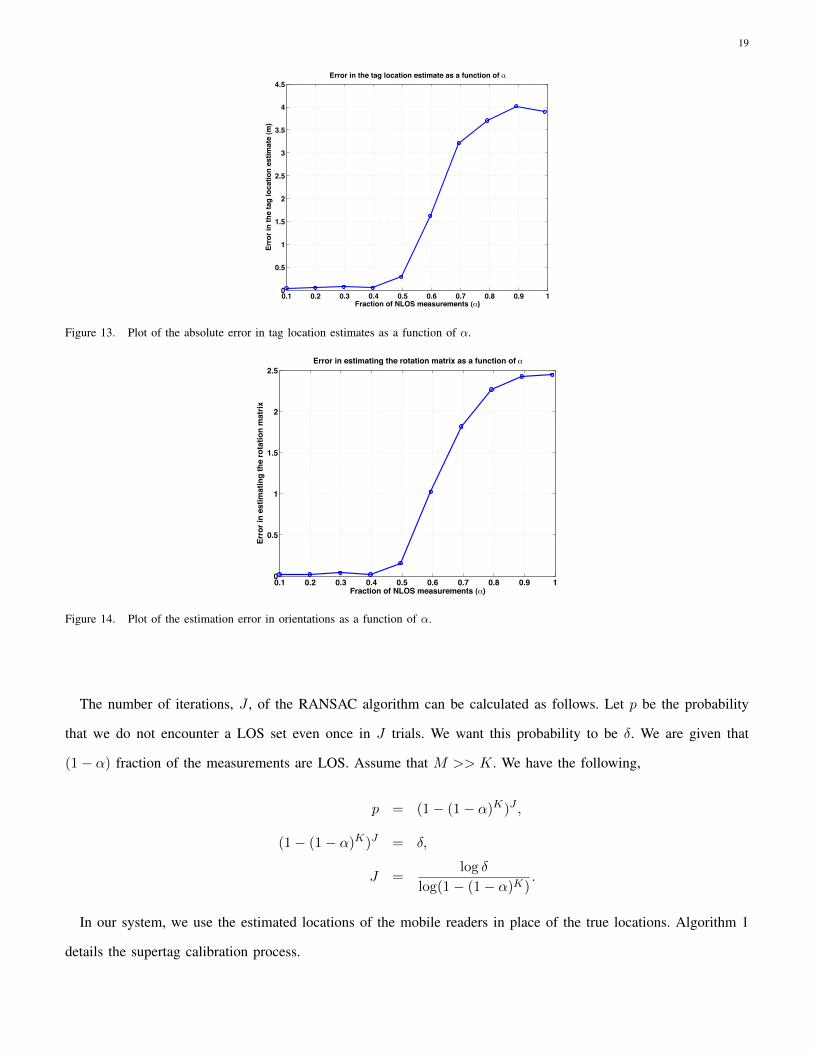
and roll angles for the supertags were taken uniformly between 0 and 20 deg. The metric for the error in estimating

the rotation matrix is taken to be ||I−RTR||F [27], which lies in the range [0, 2√

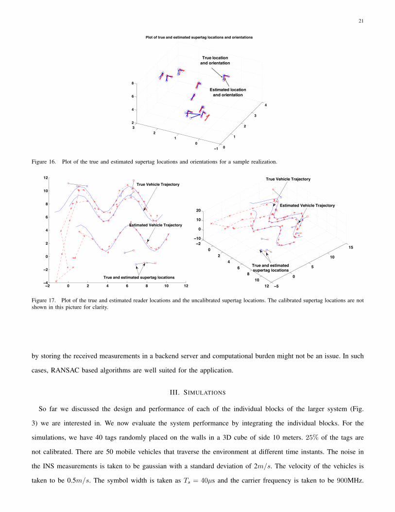
2]. Fig. 16 shows a visualization

of a single realization of the true and estimated supertag locations and orientations in the case when α = 0.4. Fig.

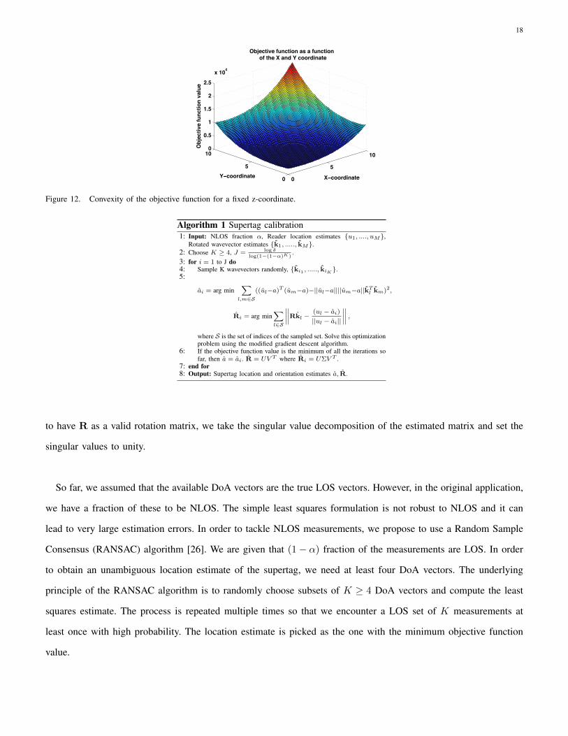
13 and 14 show plots of the error in localization and orientation as a function of the fraction of NLOS measurements.

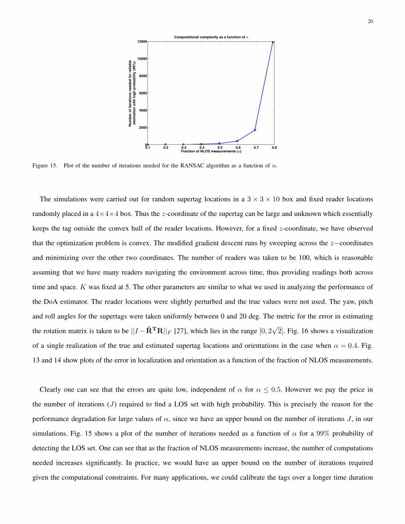
Clearly one can see that the errors are quite low, independent of α for α ≤ 0.5. However we pay the price in

the number of iterations (J) required to find a LOS set with high probability. This is precisely the reason for the

performance degradation for large values of α, since we have an upper bound on the number of iterations J , in our

simulations. Fig. 15 shows a plot of the number of iterations needed as a function of α for a 99% probability of

detecting the LOS set. One can see that as the fraction of NLOS measurements increase, the number of computations

needed increases significantly. In practice, we would have an upper bound on the number of iterations required

given the computational constraints. For many applications, we could calibrate the tags over a longer time duration

21

0

1

2

3

4

10

12

32

4

6

8

Plot of true and estimated supertag locations and orientations

Estimated locationand orientation

True locationand orientation

Figure 16. Plot of the true and estimated supertag locations and orientations for a sample realization.

2 0 2 4 6 8 10 124

2

0

2

4

6

8

10

12True Vehicle Trajectory

True and estimated supertag locations

Estimated Vehicle Trajectory

20

24

68

1012 5

0

5

10

15

10

0

10

20

True Vehicle Trajectory

Estimated Vehicle Trajectory

True and estimated supertag locations

Figure 17. Plot of the true and estimated reader locations and the uncalibrated supertag locations. The calibrated supertag locations are notshown in this picture for clarity.

by storing the received measurements in a backend server and computational burden might not be an issue. In such

cases, RANSAC based algorithms are well suited for the application.

III. SIMULATIONS

So far we discussed the design and performance of each of the individual blocks of the larger system (Fig.

3) we are interested in. We now evaluate the system performance by integrating the individual blocks. For the

simulations, we have 40 tags randomly placed on the walls in a 3D cube of side 10 meters. 25% of the tags are

not calibrated. There are 50 mobile vehicles that traverse the environment at different time instants. The noise in

the INS measurements is taken to be gaussian with a standard deviation of 2m/s. The velocity of the vehicles is

taken to be 0.5m/s. The symbol width is taken as Ts = 40µs and the carrier frequency is taken to be 900MHz.

22

0 1 2 3 4 5 6 7 8 9 100

0.1

0.2

0.3

0.4

0.5

0.6

0.7

0.8

0.9

1CDF of the localization error for different values of the LOS path gain

Error in estimating the reader location (m)

Cum

ulat

ive

dens

ity fu

nctio

n of

the

read

er lo

caliz

atio

n er

ror

LOS Gain = 1LOS Gain = 2 LOS Gain = 4

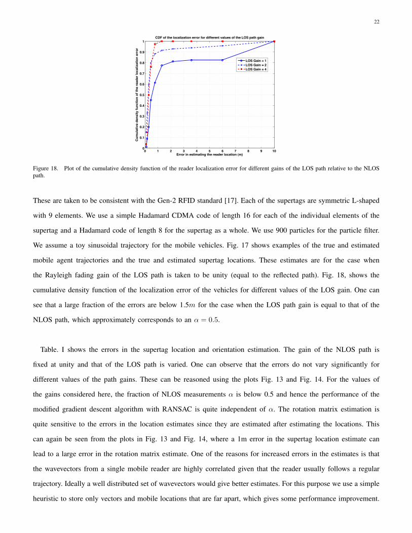
Figure 18. Plot of the cumulative density function of the reader localization error for different gains of the LOS path relative to the NLOSpath.

These are taken to be consistent with the Gen-2 RFID standard [17]. Each of the supertags are symmetric L-shaped

with 9 elements. We use a simple Hadamard CDMA code of length 16 for each of the individual elements of the

supertag and a Hadamard code of length 8 for the supertag as a whole. We use 900 particles for the particle filter.

We assume a toy sinusoidal trajectory for the mobile vehicles. Fig. 17 shows examples of the true and estimated

mobile agent trajectories and the true and estimated supertag locations. These estimates are for the case when

the Rayleigh fading gain of the LOS path is taken to be unity (equal to the reflected path). Fig. 18, shows the

cumulative density function of the localization error of the vehicles for different values of the LOS gain. One can

see that a large fraction of the errors are below 1.5m for the case when the LOS path gain is equal to that of the

NLOS path, which approximately corresponds to an α = 0.5.

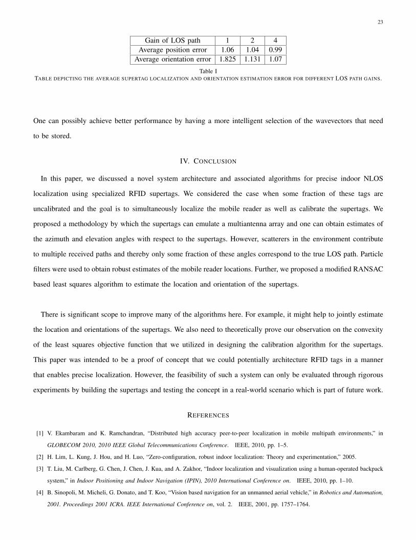
Table. I shows the errors in the supertag location and orientation estimation. The gain of the NLOS path is

fixed at unity and that of the LOS path is varied. One can observe that the errors do not vary significantly for

different values of the path gains. These can be reasoned using the plots Fig. 13 and Fig. 14. For the values of

the gains considered here, the fraction of NLOS measurements α is below 0.5 and hence the performance of the

modified gradient descent algorithm with RANSAC is quite independent of α. The rotation matrix estimation is

quite sensitive to the errors in the location estimates since they are estimated after estimating the locations. This

can again be seen from the plots in Fig. 13 and Fig. 14, where a 1m error in the supertag location estimate can

lead to a large error in the rotation matrix estimate. One of the reasons for increased errors in the estimates is that

the wavevectors from a single mobile reader are highly correlated given that the reader usually follows a regular

trajectory. Ideally a well distributed set of wavevectors would give better estimates. For this purpose we use a simple

heuristic to store only vectors and mobile locations that are far apart, which gives some performance improvement.

23

Gain of LOS path 1 2 4Average position error 1.06 1.04 0.99

Average orientation error 1.825 1.131 1.07

Table ITABLE DEPICTING THE AVERAGE SUPERTAG LOCALIZATION AND ORIENTATION ESTIMATION ERROR FOR DIFFERENT LOS PATH GAINS.

One can possibly achieve better performance by having a more intelligent selection of the wavevectors that need

to be stored.

IV. CONCLUSION

In this paper, we discussed a novel system architecture and associated algorithms for precise indoor NLOS

localization using specialized RFID supertags. We considered the case when some fraction of these tags are

uncalibrated and the goal is to simultaneously localize the mobile reader as well as calibrate the supertags. We

proposed a methodology by which the supertags can emulate a multiantenna array and one can obtain estimates of

the azimuth and elevation angles with respect to the supertags. However, scatterers in the environment contribute

to multiple received paths and thereby only some fraction of these angles correspond to the true LOS path. Particle

filters were used to obtain robust estimates of the mobile reader locations. Further, we proposed a modified RANSAC

based least squares algorithm to estimate the location and orientation of the supertags.

There is significant scope to improve many of the algorithms here. For example, it might help to jointly estimate

the location and orientations of the supertags. We also need to theoretically prove our observation on the convexity

of the least squares objective function that we utilized in designing the calibration algorithm for the supertags.

This paper was intended to be a proof of concept that we could potentially architecture RFID tags in a manner

that enables precise localization. However, the feasibility of such a system can only be evaluated through rigorous

experiments by building the supertags and testing the concept in a real-world scenario which is part of future work.

REFERENCES

[1] V. Ekambaram and K. Ramchandran, “Distributed high accuracy peer-to-peer localization in mobile multipath environments,” in

GLOBECOM 2010, 2010 IEEE Global Telecommunications Conference. IEEE, 2010, pp. 1–5.

[2] H. Lim, L. Kung, J. Hou, and H. Luo, “Zero-configuration, robust indoor localization: Theory and experimentation,” 2005.

[3] T. Liu, M. Carlberg, G. Chen, J. Chen, J. Kua, and A. Zakhor, “Indoor localization and visualization using a human-operated backpack

system,” in Indoor Positioning and Indoor Navigation (IPIN), 2010 International Conference on. IEEE, 2010, pp. 1–10.

[4] B. Sinopoli, M. Micheli, G. Donato, and T. Koo, “Vision based navigation for an unmanned aerial vehicle,” in Robotics and Automation,

2001. Proceedings 2001 ICRA. IEEE International Conference on, vol. 2. IEEE, 2001, pp. 1757–1764.

24

[5] K. Chintalapudi, A. Padmanabha Iyer, and V. Padmanabhan, “Indoor localization without the pain,” in Proceedings of the sixteenth

annual international conference on Mobile computing and networking. ACM, 2010, pp. 173–184.

[6] N. Ravi, P. Shankar, A. Frankel, A. Elgammal, and L. Iftode, “Indoor localization using camera phones,” in Mobile Computing Systems

and Applications, 2006. WMCSA’06. Proceedings. 7th IEEE Workshop on. Ieee, 2006, pp. 49–49.

[7] V. Otsason, A. Varshavsky, A. LaMarca, and E. De Lara, “Accurate gsm indoor localization,” UbiComp 2005: Ubiquitous Computing,

pp. 903–903, 2005.

[8] J. Gutmann and C. Schlegel, “Amos: Comparison of scan matching approaches for self-localization in indoor environments,” in Advanced

Mobile Robot, 1996., Proceedings of the First Euromicro Workshop on. IEEE, 1996, pp. 61–67.

[9] Y. Chen, J. Francisco, W. Trappe, and R. Martin, “A practical approach to landmark deployment for indoor localization,” in Sensor

and Ad Hoc Communications and Networks, 2006. SECON’06. 2006 3rd Annual IEEE Communications Society on, vol. 1. IEEE,

2006, pp. 365–373.

[10] N. Priyantha, “The cricket indoor location system,” Ph.D. dissertation, Massachusetts Institute of Technology, 2005.

[11] Nokia. (2010) Nokia high accuracy indoor positioning technology. [Online]. Available: http://research.nokia.com/news/9505

[12] K. Finkenzeller et al., RFID Handbook: Fundamentals and applications in contactless smart cards, radio frequency identification and

near-field communication. Wiley, 2010.

[13] L. Ni, Y. Liu, Y. Lau, and A. Patil, “Landmarc: indoor location sensing using active rfid,” Wireless networks, vol. 10, no. 6, pp. 701–710,

2004.

[14] M. Bouet and A. Dos Santos, “Rfid tags: Positioning principles and localization techniques,” in Wireless Days, 2008. WD’08. 1st IFIP.

Ieee, 2008, pp. 1–5.

[15] D. Hahnel, W. Burgard, D. Fox, K. Fishkin, and M. Philipose, “Mapping and localization with rfid technology,” in Robotics and

Automation, 2004. Proceedings. ICRA’04. 2004 IEEE International Conference on, vol. 1. IEEE, 2004, pp. 1015–1020.

[16] J. Griffin and G. Durgin, “Multipath fading measurements for multi-antenna backscatter rfid at 5.8 ghz,” in RFID, 2009 IEEE

International Conference on. IEEE, 2009, pp. 322–329.

[17] M. O’Connor, “Gen 2 epc protocol approved as iso 18000-6c,” RFID Journal, vol. 1, no. 11, 2006.

[18] C. Mutti and C. Floerkemeier, “Cdma-based rfid systems in dense scenarios: Concepts and challenges,” in RFID, 2008 IEEE International

Conference on. IEEE, 2008, pp. 215–222.

[19] P. Stoica and R. Moses, Introduction to spectral analysis. Prentice Hall Upper Saddle River, NJ, 1997, vol. 51.

[20] M. Jordan, “Graphical models,” Statistical Science, pp. 140–155, 2004.

[21] G. Welch and G. Bishop, “An introduction to the kalman filter,” Design, vol. 7, no. 1, pp. 1–16, 2001.

[22] E. Wan and R. Van Der Merwe, “The unscented kalman filter for nonlinear estimation,” in Adaptive Systems for Signal Processing,

Communications, and Control Symposium 2000. AS-SPCC. The IEEE 2000. IEEE, 2000, pp. 153–158.

[23] M. Arulampalam, S. Maskell, N. Gordon, and T. Clapp, “A tutorial on particle filters for online nonlinear/non-gaussian bayesian

tracking,” Signal Processing, IEEE Transactions on, vol. 50, no. 2, pp. 174–188, 2002.

[24] T. Moon, “The expectation-maximization algorithm,” Signal Processing Magazine, IEEE, vol. 13, no. 6, pp. 47–60, 1996.

[25] E. Weisstein, CRC concise encyclopedia of mathematics. CRC Pr I Llc, 2003.

[26] M. Fischler and R. Bolles, “Random sample consensus: a paradigm for model fitting with applications to image analysis and automated

cartography,” Communications of the ACM, vol. 24, no. 6, pp. 381–395, 1981.

[27] D. Huynh, “Metrics for 3d rotations: Comparison and analysis,” Journal of Mathematical Imaging and Vision, vol. 35, no. 2, pp.

155–164, 2009.