A Framework for Simultaneous Localization andMapping Utilizing Model Structure

Thomas B. Schon, Rickard Karlsson, David Tornqvist, and Fredrik GustafssonDivision of Automatic Control

Department of Electrical EngineeringLinkoping University

SE–581 83 Linkoping, SwedenEmail: {schon, rickard, tornqvist, fredrik}@isy.liu.se

Abstract—This contribution aims at unifying two recent trendsin applied particle filtering (PF). The first trend is the majorimpact in simultaneous localization and mapping (SLAM) ap-plications, utilizing the FastSLAM algorithm. The second oneis the implications of the marginalized particle filter (MPF) orthe Rao-Blackwellized particle filter (RBPF) in positioning andtracking applications. An algorithm is introduced, which mergesFastSLAM and MPF, and the result is an MPF algorithm forSLAM applications, where state vectors of higher dimensionscan be used. Results using experimental data from a 3D SLAMdevelopment environment, fusing measurements from inertialsensors (accelerometer and gyro) and vision are presented.

Keywords: Rao-Blackwellized/marginalized particle filter,sensor fusion, simultaneous localization and mapping,inertial sensors, vision.

I. INTRODUCTION

The main task in localization/positioning and tracking isto estimate, for instance, the position and orientation of theobject under consideration. The particle filter (PF), [1], [2],has proven to be an enabling technology for many applicationsof this kind, in particular when the observations are com-plicated nonlinear functions of the position and heading [3].Furthermore, the Rao-Blackwellized particle filter (RBPF) alsodenoted the marginalized particle filter (MPF), [4]–[9] enablesestimation of velocity, acceleration, and sensor error models byutilizing any linear Gaussian sub-structure in the model, whichis fundamental for performance in applications as surveyedin [10]. As described in [9], the MPF splits the state vectorxt into two parts, one part xp

t which is estimated using theparticle filter and another part xk

t where Kalman filters areapplied. Basically, it uses the following factorization of theposterior distribution of the state vector, which follows fromBayes’ rule,

p(xp1:t, x

kt |y1:t) = p(xk

t |xp1:t, y1:t)p(xp

1:t|y1:t), (1)

where y1:t , {y1, . . . , yt} denotes the measurements up totime t. If the model is conditionally linear Gaussian, i.e., ifthe term p(xk

t |xp1:t, y1:t) is linear Gaussian, it can be optimally

estimated using the Kalman filter, whereas for the secondfactor we have to resort to the PF.

Simultaneous localization and mapping (SLAM) is an ex-tension of the localization or positioning problem to the casewhere the environment is un-modeled and has to be mappedon-line. An introduction to the SLAM problem is given inthe survey papers [11], [12] and the recent book [13]. Froma sensor point of view, there are two ways of tackling thisproblem. The first way is to use only one sensor, such asvision, see e.g., [14]–[17] and the second way is to fusemeasurements from several sensors. This work considers thelatter.

The FastSLAM algorithm introduced in [18] has proven tobe an enabling technology for such applications. FastSLAM

can be seen as a special case of RBPF/MPF, where the mapstate mt, containing the positions for all landmarks used inthe mapping, can be interpreted as a linear Gaussian state.The main difference is that the map vector is a constantparameter with a dimension increasing over time, rather thana time-varying state with a dynamic evolution over time. Thederivation is completely analogous to (1), and makes use ofthe following factorization

p(x1:t,mt|y1:t) = p(mt|x1:t, y1:t)p(x1:t|y1:t). (2)

The FastSLAM algorithm was originally devised to solve theSLAM problem for mobile robots, where the dimension ofthe state vector is small, typically consisting of three states(2D position and a heading angle) [13]. This implies that allplatform states can be estimated by the PF.

Parallelling the evolution of PF applications to high di-mensional state vectors, the aim of this contribution is tounify the ideas presented in [9], [19] in order to extendthe FastSLAM [18] algorithm to be able to cope with highdimensional state vectors as well. Basically, the main resultfollows from

p(xp1:t,x

kt ,mt|y1:t)

= p(mt|xkt , xp

1:t, y1:t)p(xkt |x

p1:t, y1:t)p(xp

1:t|y1:t). (3)

The derived algorithm is applied to experimental data from adevelopment environment tailored to provide accurate valuesof ground truth. Here, a high precision industrial robot isprogrammed to move, possibly using its 6 degrees-of-freedom

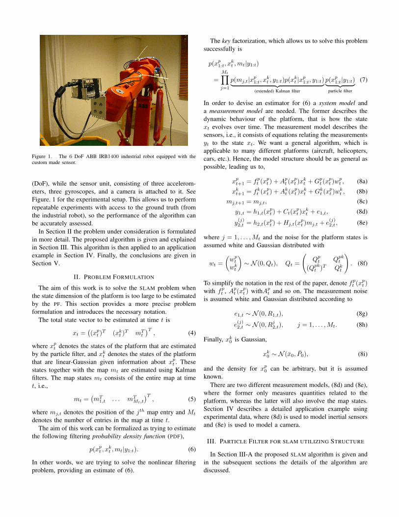
Figure 1. The 6 DoF ABB IRB1400 industrial robot equipped with thecustom made sensor.

(DoF), while the sensor unit, consisting of three accelerom-eters, three gyroscopes, and a camera is attached to it. SeeFigure. 1 for the experimental setup. This allows us to performrepeatable experiments with access to the ground truth (fromthe industrial robot), so the performance of the algorithm canbe accurately assessed.

In Section II the problem under consideration is formulatedin more detail. The proposed algorithm is given and explainedin Section III. This algorithm is then applied to an applicationexample in Section IV. Finally, the conclusions are given inSection V.

II. PROBLEM FORMULATION

The aim of this work is to solve the SLAM problem whenthe state dimension of the platform is too large to be estimatedby the PF. This section provides a more precise problemformulation and introduces the necessary notation.

The total state vector to be estimated at time t is

xt =((xp

t )T (xkt )T mT

t

)T, (4)

where xpt denotes the states of the platform that are estimated

by the particle filter, and xkt denotes the states of the platform

that are linear-Gaussian given information about xpt . These

states together with the map mt are estimated using Kalmanfilters. The map states mt consists of the entire map at timet, i.e.,

mt =(mT

1,t . . . mTMt,t

)T, (5)

where mj,t denotes the position of the jth map entry and Mt

denotes the number of entries in the map at time t.The aim of this work can be formalized as trying to estimate

the following filtering probability density function (PDF),

p(xpt , x

kt ,mt|y1:t). (6)

In other words, we are trying to solve the nonlinear filteringproblem, providing an estimate of (6).

The key factorization, which allows us to solve this problemsuccessfully is

p(xp1:t, x

kt ,mt|y1:t)

=Mt∏j=1

p(mj,t|xp1:t, x

kt , y1:t)p(xk

t |xp1:t, y1:t)︸ ︷︷ ︸

(extended) Kalman filter

p(xp1:t|y1:t)︸ ︷︷ ︸

particle filter

(7)

In order to devise an estimator for (6) a system model anda measurement model are needed. The former describes thedynamic behaviour of the platform, that is how the statext evolves over time. The measurement model describes thesensors, i.e., it consists of equations relating the measurementsyt to the state xt. We want a general algorithm, which isapplicable to many different platforms (aircraft, helicopters,cars, etc.). Hence, the model structure should be as general aspossible, leading us to,

xpt+1 = fp

t (xpt ) + Ap

t (xpt )x

kt + Gp

t (xpt )w

pt , (8a)

xkt+1 = fk

t (xpt ) + Ak

t (xpt )x

kt + Gk

t (xpt )w

kt , (8b)

mj,t+1 = mj,t, (8c)

y1,t = h1,t(xpt ) + Ct(x

pt )x

kt + e1,t, (8d)

y(j)2,t = h2,t(x

pt ) + Hj,t(x

pt )mj,t + e

(j)2,t , (8e)

where j = 1, . . . ,Mt and the noise for the platform states isassumed white and Gaussian distributed with

wt =(

wpt

wkt

)∼ N (0, Qt), Qt =

(Qp

t Qpkt

(Qpkt )T Qk

t

). (8f)

To simplify the notation in the rest of the paper, denote fpt (xp

t )with fp

t , Apt (x

pt ) withAp

t and so on. The measurement noiseis assumed white and Gaussian distributed according to

e1,t ∼ N (0, R1,t), (8g)

e(j)2,t ∼ N (0, Rj

2,t), j = 1, . . . ,Mt. (8h)

Finally, xk0 is Gaussian,

xk0 ∼ N (x0, P0), (8i)

and the density for xp0 can be arbitrary, but it is assumed

known.There are two different measurement models, (8d) and (8e),

where the former only measures quantities related to theplatform, whereas the latter will also involve the map states.Section IV describes a detailed application example usingexperimental data, where (8d) is used to model inertial sensorsand (8e) is used to model a camera.

III. PARTICLE FILTER FOR SLAM UTILIZING STRUCTURE

In Section III-A the proposed SLAM algorithm is given andin the subsequent sections the details of the algorithm arediscussed.

A. Algorithm

The algorithm presented in this paper draws on severalrather well known algorithms. It is based on the RBPF/MPF

method, [4]–[9]. The FastSLAM algorithm [18] is extendedby not only including the map states, but also the statescorresponding to a linear Gaussian sub-structure present in themodel for the platform. Assuming that the platform is modeledin the form given in (8), the SLAM-method utilizing structureis given in Algorithm 1.

Algorithm 1: Particle filter for SLAM utilizing structure

1) Initialize the particles

xp,(i)1|0 ∼ p(xp

1|0),

xk,(i)1|0 = xk

1|0,

Pk,(i)1|0 = P1|0, i = 1, . . . , N,

where N denotes the number of particles.2) If there is a new map related measurement available

perform data association for each particle, otherwiseproceed to step 3.

3) Compute the importance weights according to

γ(i)t = p(yt|xp,(i)

1:t , y1:t−1), i = 1, . . . , N,

and normalize γ(i)t = γ

(i)t /

∑Nj=1 γ

(j)t .

4) Draw N new particles with replacement (resam-pling) according to, for each i = 1, . . . , N

Pr(x(i)t|t = x

(j)t|t ) = γ

(j)t , j = 1, . . . , N.

5) If there is a new map related measurement, performmap estimation and management (detailed below),otherwise proceed to step 6.

6) Particle filter prediction and Kalman filter (for eachparticle i = 1, . . . , N )

a) Kalman filter measurement update,

p(xkt |x

p1:t, y1:t) = N (xk

t |xk,(i)t|t , P

(i)t|t ),

where xk,(i)t|t and P

(i)t|t are given in (11).

b) Time update for the nonlinear particles,

xp,(i)t+1|t ∼ p(xt+1|t|x

p,(i)1:t , y1:t).

c) Kalman filter time update,

p(xkt+1|x

p1:t+1, y1:t)

= N (xkt+1|t|x

k,(i)t+1|t, P

(i)t+1|t),

where xk,(i)t+1|t and P

(i)t+1|t are given by (12).

7) Set t := t + 1 and iterate from step 2.

Note that yt denotes the measurements present at time t. Thefollowing theorem will give all the details for how to computethe Kalman filtering quantities. It is important to stress that

all embellishments available for the particle filter can be usedtogether with Algorithm 1. To give one example, the so-calledFastSLAM 2.0 makes use of an improved proposal distributionin step 6b [20].

Theorem 1: Using the model given by (8), the conditionalprobability density functions for xk

t and xkt+1 are given by

p(xkt |x

p1:t, y1:t) = N (xk

t|t, Pt|t), (10a)

p(xkt+1|x

p1:t+1, y1:t) = N (xk

t+1|t, Pt+1|t), (10b)

where

xkt|t = xk

t|t−1 + Kt(y1,t − h1,t − Ctxkt|t−1), (11a)

Pt|t = Pt|t−1 −KtS1,tKTt , (11b)

S1,t = CtPt|t−1CTt + R1,t, (11c)

Kt = Pt|t−1CTt S−1

1,t , (11d)

and

xkt+1|t = Ak

t xkt|t + Gk

t (Qkpt )T (Gp

t Qpt )−1zt

+ fkt + Lt(zt −Ap

t xkt|t), (12a)

Pt+1|t = Akt Pt|t(Ak

t )T + Gkt Qk

t (Gkt )T − LtS2,tL

Tt , (12b)

S2,t = Apt Pt|t(A

pt )

T + Gpt Q

pt (G

pt )

T , (12c)

Lt = Akt Pt|t(A

pt )

T S−12,t , (12d)

where

zt = xpt+1 − fp

t , (13a)

Akt = Ak

t −Gkt (Qkp

t )T (Gpt Q

pt )−1Ap

t , (13b)

Qkt = Qk

t − (Qkpt )T (Qp

t )−1Qkp

t . (13c)

Proof: See [9].

B. Data Association

Data association is a complicated problem, but it hasbeen studied extensively in the literature for many trackingapplications, see e.g., [21]–[23]. Classical methods such asthe nearest neighbor (NN), probabilistic data association(PDA), joint probabilistic data association (JPDA) or multi-hypothesis tracking (MHT) exist for single and multiple tar-gets. Depending on the number of targets, the false alarmrate and the probability of detection, these methods variesin performance and ability to express these phenomena. Themethods mentioned above were originally developed to beused together with estimators based on Kalman filters. The useof particle filters opens up for other data association methods,typically more integrated with the filter.

The particle implementation of the SLAM problem will leadto an increased complexity for the data association. This isbecause for each particle in the filter there exist several mapentries. Hence, many classical association methods will be toocomputationally intensive for a direct implementation.

C. Likelihood Computation

In order to compute the importance weights {γ(i)t }N

i=1 inAlgorithm 1, the following likelihoods have to be evaluated

γ(i)t = p(yt|xp,(i)

1:t , y1:t−1), i = 1, . . . , N. (14)

The standard way of performing this type of computationis simply to marginalize the Kalman filter variables xk

t and{mj,t}Mt

j=1,

p(yt|xp,(i)1:t , y1:t−1) =

∫p(yt, x

kt ,mt|xp,(i)

1:t , y1:t−1)dxkt dmt,

(15)

where

p(yt, xkt ,mt|xp,(i)

1:t , y1:t−1) = p(yt|xkt ,mt, x

p,(i)t )×

p(xkt |x

p,(i)1:t , y1:t−1)

Mt∏j=1

p(mj,t|xp,(i)1:t , y1:t−1).

(16)

Let us consider the case where both y1,t and y2,t are present,i.e., yt =

(yT1,t yT

2,t

)T. Note that the cases where either y1,t

or y2,t are present are obviously special cases. First of all, themeasurements are conditionally independent given the state,implying that

p(yt|xkt ,mt, x

p,(i)t ) = p(y1,t|xk

t , xp,(i)t )

Mt∏j=1

p(y(j)2,t |x

p,(i)t ,mj,t).

(17)

Now, inserting (17) into (16) gives

p(yt, xkt ,mt|xp,(i)

1:t , y1:t−1) =

p(y1,t|xkt , x

p,(i)t )p(xk

t |xp,(i)1:t , y1:t−1)×

Mt∏j=1

p(mj,t|xp,(i)1:t , y1:t−1)p(y(j)

2,t |xp,(i)t ,mj,t), (18)

which inserted in (15) finally results in

p(yt|xp,(i)1:t , y1:t−1) =

∫p(y1,t|xk

t , xp,(i)t )p(xk

t |xp,(i)1:t , y1:t−1)dxk

t

×Mt∏j=1

∫p(y

(j)2,t |x

p,(i)t , mj,t)p(mj,t|xp,(i)

1:t , y1:t−1)dm1,t · · · dmMt,t.

(19)

All the densities present in (19) are known according to

p(xkt |x

p1:t, y1:t−1) = N (xk

t |xkt|t−1, Pt|t−1), (20a)

p(mj,t|xp1:t, y1:t−1) = N (mt|mj,t−1,Σt−1), (20b)

p(y1,t|xkt , xp

t ) = N (y1,t|h1,t + Ctxkt , R1), (20c)

p(y(j)2,t |x

pt ,mj,t) = N (y(j)

2,t |h2,t + Hj,tmj,t, Rj2). (20d)

Here it is important to note that the standard FastSLAM

approximation has been invoked in order to obtain (20d). Thatis, the measurement equation (8e) is linearized with respect tothe map states mj,t. The reason for this approximation is thatwe for computational reasons want to use a model suitable

for the RBPF/MPF, otherwise the dimension will be much toolarge for the particle filter to handle. Using (20), the integralsin (19) can now be solved, resulting in

p(yt|xp,(i)1:t , y1:t−1) =

N (y1,t − h1,t − Ctxk,(i)t|t−1, CtP

(i)t|t−1C

Tt )

×Mt∏j=1

N (y(j)2,t−h2,t−Hj,tmj,t−1,Hj,tΣj,t−1(Hj,t)T +Rj

2).

(21)

D. Map Estimation and Map Management

A simple map consists of a collection of map point entries{mj,t}Mt

j=1, each consisting of:• mj,t – estimate of the position (three dimensions).

• Σj,t – covariance for the position estimate.Note that this is a very simple map parameterization. Eachparticle has an entire map estimate associated to it. Step 5of Algorithm 1 consists of updating these map estimates inaccordance with the new map-related measurements that areavailable. First of all, if a measurement has been successfullyassociated to a certain map entry, it is updated using thestandard Kalman filter measurement update according to

mj,t = mj,t−1 + Kj,t

(y(j)2,t − h2,t

), (22a)

Σj,t =(I −Kj,tH

Ti,t

)Σj,t−1, (22b)

Kj,t = Σj,t−1Hj,t

(Hj,tΣj,t−1H

Tj,t + R2

)−1. (22c)

If an existing map entry is not observed, the correspondingmap estimate is simply propagated according to its dynamics,i.e., it is unchanged

mj,t = mj,t−1, (23a)

Σj,t = Σj,t−1. (23b)

It has to be checked if any of the entries should be removedfrom the map.

Finally, initialization of new map entries have to be handled.If h2,t(x

pt ,mj,t) is bijective with respect to the map mj,t

this can be used to directly initialize the position from themeasurement y2,t. However, this is typically not the case,implying that there is a need for more than one measurementin order to be able to initialize a new map entry, utilizing forexample triangulation.

E. Approximate Algorithm

The computational complexity of Algorithm 1 will in-evitably be high, implying that it is interesting to considerideas on how to reduce it. In the present context multi-rate sensors (sensors providing measurements with differentsampling times) are typically used. This can be exploited ina way similar to that in [19]. The idea is that, rather thanrunning Algorithm 1 at the same frequency as the fast sensor,it is executed at the same frequency as the slow sensor, with

a nested filter handling the fast sensor measurements. Thisapproach involves approximations.

In this way both the linear Gaussian sub-structure in theplatform model and the multi-rate properties of the sensorsare exploited in order to obtain an efficient algorithm [19].

IV. APPLICATION EXAMPLE

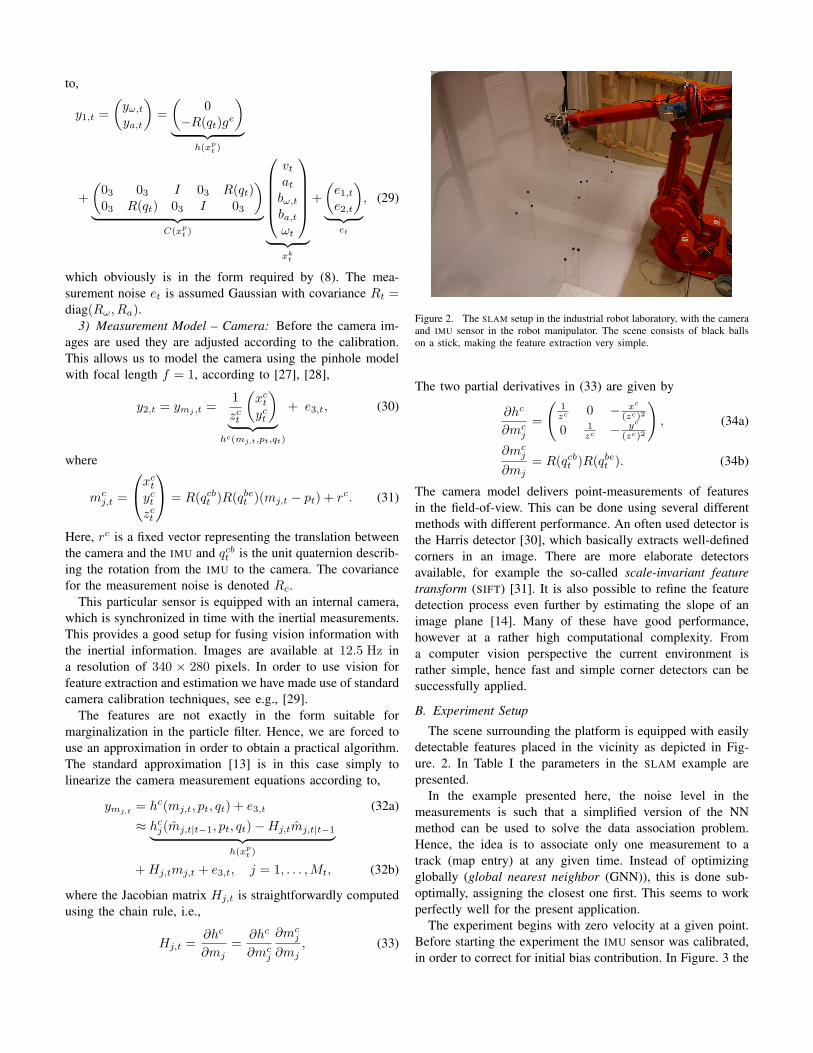
In this section we provide a rather detailed treatment ofa SLAM application, where Algorithm 1 is used to fusemeasurements from a camera, three accelerometers and threegyroscopes. The sensor has been attached to a high precision6 DoF ABB IRB1440 industrial robot. The reason for thisis that the robot will allow us to make repeatable 6 DoFmotions and it will provide the true position and orientationwith very high accuracy. This enables systematic evaluationof algorithms. The sensor and its mounting to the industrialrobot is illustrated in Figure. 1.

The main objective is to find the position and orientationof the sensor from sensor data only, despite problems such asbiases in the measurements. In the surrounding neighbourhoodfeatures are placed in such a way that the vision system caneasily extract features. These are used in SLAM to reduce theproblem caused by inertial drift and bias in the IMU sensor.

A. Model

The basic part of the state vector consists of positionpt ∈ R3, velocity vt ∈ R3, and acceleration at ∈ R3,all described in an earth-fixed reference frame. Furthermore,the state vector is extended with bias states for accelerationba,t ∈ R3, and angular velocity bω,t ∈ R3 in order to accountfor sensor imperfections. The state vector also contains theangular velocity ωt and a unit quaternion qt, which is used toparameterize the orientation.

In order to put the model in the RBPF/MPF framework, thestate vector is split into two parts, one estimated using Kalmanfilters xk

t and one estimated using the particle filter xpt . Hence,

define

xkt =

(vT

t aTt (bω,t)T (ba,t)T ωT

t

)T, (24a)

xpt =

(pT

t qTt

)T, (24b)

which means xkt ∈ R15 and xp

t ∈ R7. In inertial estimation itis essential to clearly state which coordinate system any entityis expressed in. Here the notation is simplified by suppressingthe coordinate system for the earth-fixed states, which meansthat

pt = pet , vt = ve

t , at = aet , (25a)

wt = wet , bω,t = bb

ω,t, ba,t = bba,t. (25b)

Likewise, the unit quaternions represent the rotation from theearth-fixed system to the body (IMU) system, since the IMU isrigidly attached to the body (strap-down),

qt = qbet =

(qt,0 qt,1 qt,2 qt,3

)T. (26)

The quaternion estimates are normalized, to make sure thatthey still parameterizes an orientation. Further details re-garding orientation and coordinate systems are given in Ap-pendix A.

1) Dynamic Model: The dynamic model describes how theplatform and the map evolve over time. These equations aregiven below, in the form (8a) – (8d), suitable for direct use inAlgorithm 1.

vt+1

at+1

bω,t+1

ba,t+1

ωt+1

︸ ︷︷ ︸

xkt+1

=

I TI 0 0 00 I 0 0 00 0 I 0 00 0 0 I 00 0 0 0 I

︸ ︷︷ ︸

Akt

vt

at

bω,t

ba,t

ωt

︸ ︷︷ ︸

xkt

+

0 0 0 0I 0 0 00 I 0 00 0 I 00 0 0 I

︸ ︷︷ ︸

Gkt

w1,t

w2,t

w3,t

w4,t

︸ ︷︷ ︸

wkt

(27a)

(pt+1

qt+1

)︸ ︷︷ ︸

xpt+1

=(

pt

qt

)︸ ︷︷ ︸fp

t (xpt )

+

(TI T 2

2 I 03×9

04×3 04×9 −T2 S(q)

)︸ ︷︷ ︸

Apt (xp

t )

vt

at

bω,t

ba,t

ωt

︸ ︷︷ ︸

xkt

+wpt ,

(27b)

mj,t+1 = mj,t, j = 1, . . . ,Mt, (27c)

where

S(q) =

−q1 −q2 −q3

q0 q3 −q2

−q3 q0 q1

q2 −q1 q0

, (28)

and where I denotes the 3 × 3 unit matrix and 0 denotesthe 3 × 3 zero matrix, unless otherwise stated. The processnoise wk

t is assumed to be independent and Gaussian, withcovariance Qk

t = diag(Qa, Qbω, Qba

, Qω).2) Measurement Model – Inertial Sensors: The IMU con-

sists of accelerometers measuring accelerations ya,t in all threedimensions, a gyroscope measuring angular velocities yω,t inthree dimensions and a magnetometer measuring the directionto the magnetic north pole. Due to the fairly magnetic environ-ment it is just the accelerometers and gyroscopes that are usedfor positioning. The inertial sensors operate at 100 Hz. Forfurther details on inertial sensors, see for instance [24]–[26].The inertial measurements are related to the states according

to,

y1,t =(

yω,t

ya,t

)=(

0−R(qt)ge

)︸ ︷︷ ︸

h(xpt )

+(

03 03 I 03 R(qt)03 R(qt) 03 I 03

)︸ ︷︷ ︸

C(xpt )

vt

at

bω,t

ba,t

ωt

︸ ︷︷ ︸

xkt

+(

e1,t

e2,t

)︸ ︷︷ ︸

et

, (29)

which obviously is in the form required by (8). The mea-surement noise et is assumed Gaussian with covariance Rt =diag(Rω, Ra).

3) Measurement Model – Camera: Before the camera im-ages are used they are adjusted according to the calibration.This allows us to model the camera using the pinhole modelwith focal length f = 1, according to [27], [28],

y2,t = ymj ,t =1zct

(xc

t

yct

)︸ ︷︷ ︸

hc(mj,t,pt,qt)

+ e3,t, (30)

where

mcj,t =

xct

yct

zct

= R(qcbt )R(qbe

t )(mj,t − pt) + rc. (31)

Here, rc is a fixed vector representing the translation betweenthe camera and the IMU and qcb

t is the unit quaternion describ-ing the rotation from the IMU to the camera. The covariancefor the measurement noise is denoted Rc.

This particular sensor is equipped with an internal camera,which is synchronized in time with the inertial measurements.This provides a good setup for fusing vision information withthe inertial information. Images are available at 12.5 Hz ina resolution of 340 × 280 pixels. In order to use vision forfeature extraction and estimation we have made use of standardcamera calibration techniques, see e.g., [29].

The features are not exactly in the form suitable formarginalization in the particle filter. Hence, we are forced touse an approximation in order to obtain a practical algorithm.The standard approximation [13] is in this case simply tolinearize the camera measurement equations according to,

ymj,t = hc(mj,t, pt, qt) + e3,t (32a)

≈ hcj(mj,t|t−1, pt, qt)−Hj,tmj,t|t−1︸ ︷︷ ︸

h(xpt )

+ Hj,tmj,t + e3,t, j = 1, . . . ,Mt, (32b)

where the Jacobian matrix Hj,t is straightforwardly computedusing the chain rule, i.e.,

Hj,t =∂hc

∂mj=

∂hc

∂mcj

∂mcj

∂mj, (33)

Figure 2. The SLAM setup in the industrial robot laboratory, with the cameraand IMU sensor in the robot manipulator. The scene consists of black ballson a stick, making the feature extraction very simple.

The two partial derivatives in (33) are given by

∂hc

∂mcj

=

(1zc 0 − xc

(zc)2

0 1zc − yc

(zc)2

), (34a)

∂mcj

∂mj= R(qcb

t )R(qbet ). (34b)

The camera model delivers point-measurements of featuresin the field-of-view. This can be done using several differentmethods with different performance. An often used detector isthe Harris detector [30], which basically extracts well-definedcorners in an image. There are more elaborate detectorsavailable, for example the so-called scale-invariant featuretransform (SIFT) [31]. It is also possible to refine the featuredetection process even further by estimating the slope of animage plane [14]. Many of these have good performance,however at a rather high computational complexity. Froma computer vision perspective the current environment israther simple, hence fast and simple corner detectors can besuccessfully applied.

B. Experiment Setup

The scene surrounding the platform is equipped with easilydetectable features placed in the vicinity as depicted in Fig-ure. 2. In Table I the parameters in the SLAM example arepresented.

In the example presented here, the noise level in themeasurements is such that a simplified version of the NNmethod can be used to solve the data association problem.Hence, the idea is to associate only one measurement to atrack (map entry) at any given time. Instead of optimizingglobally (global nearest neighbor (GNN)), this is done sub-optimally, assigning the closest one first. This seems to workperfectly well for the present application.

The experiment begins with zero velocity at a given point.Before starting the experiment the IMU sensor was calibrated,in order to correct for initial bias contribution. In Figure. 3 the

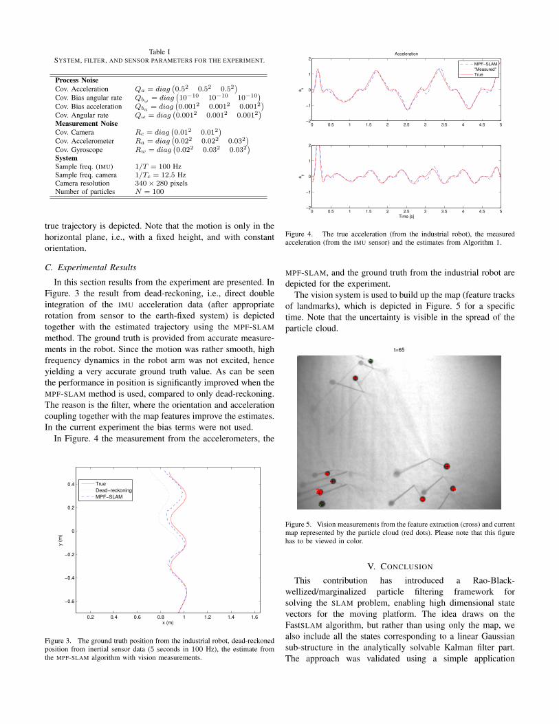
Table ISYSTEM, FILTER, AND SENSOR PARAMETERS FOR THE EXPERIMENT.

Process NoiseCov. Acceleration Qa = diag

(0.52 0.52 0.52

)Cov. Bias angular rate Qbω = diag

(10−10 10−10 10−10

)Cov. Bias acceleration Qba = diag

(0.0012 0.0012 0.0012

)Cov. Angular rate Qω = diag

(0.0012 0.0012 0.0012

)Measurement NoiseCov. Camera Rc = diag

(0.012 0.012

)Cov. Accelerometer Ra = diag

(0.022 0.022 0.032

)Cov. Gyroscope Rw = diag

(0.022 0.032 0.032

)SystemSample freq. (IMU) 1/T = 100 HzSample freq. camera 1/Tc = 12.5 HzCamera resolution 340× 280 pixelsNumber of particles N = 100

true trajectory is depicted. Note that the motion is only in thehorizontal plane, i.e., with a fixed height, and with constantorientation.

C. Experimental Results

In this section results from the experiment are presented. InFigure. 3 the result from dead-reckoning, i.e., direct doubleintegration of the IMU acceleration data (after appropriaterotation from sensor to the earth-fixed system) is depictedtogether with the estimated trajectory using the MPF-SLAM

method. The ground truth is provided from accurate measure-ments in the robot. Since the motion was rather smooth, highfrequency dynamics in the robot arm was not excited, henceyielding a very accurate ground truth value. As can be seenthe performance in position is significantly improved when theMPF-SLAM method is used, compared to only dead-reckoning.The reason is the filter, where the orientation and accelerationcoupling together with the map features improve the estimates.In the current experiment the bias terms were not used.

In Figure. 4 the measurement from the accelerometers, the

0.2 0.4 0.6 0.8 1 1.2 1.4 1.6

−0.6

−0.4

−0.2

0

0.2

0.4

x (m)

y (

m)

True

Dead−reckoning

MPF−SLAM

Figure 3. The ground truth position from the industrial robot, dead-reckonedposition from inertial sensor data (5 seconds in 100 Hz), the estimate fromthe MPF-SLAM algorithm with vision measurements.

0 0.5 1 1.5 2 2.5 3 3.5 4 4.5 5−2

−1

0

1

2Acceleration

ax

0 0.5 1 1.5 2 2.5 3 3.5 4 4.5 5−2

−1

0

1

2

ay

Time [s]

MPF−SLAM

"Measured"

True

Figure 4. The true acceleration (from the industrial robot), the measuredacceleration (from the IMU sensor) and the estimates from Algorithm 1.

MPF-SLAM, and the ground truth from the industrial robot aredepicted for the experiment.

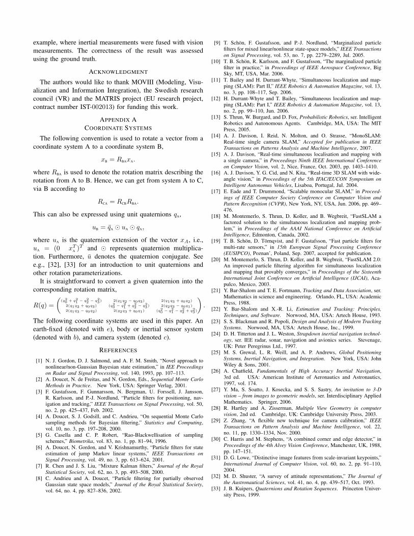
The vision system is used to build up the map (feature tracksof landmarks), which is depicted in Figure. 5 for a specifictime. Note that the uncertainty is visible in the spread of theparticle cloud.

t=65

Figure 5. Vision measurements from the feature extraction (cross) and currentmap represented by the particle cloud (red dots). Please note that this figurehas to be viewed in color.

V. CONCLUSION

This contribution has introduced a Rao-Black-wellized/marginalized particle filtering framework forsolving the SLAM problem, enabling high dimensional statevectors for the moving platform. The idea draws on theFastSLAM algorithm, but rather than using only the map, wealso include all the states corresponding to a linear Gaussiansub-structure in the analytically solvable Kalman filter part.The approach was validated using a simple application

example, where inertial measurements were fused with visionmeasurements. The correctness of the result was assessedusing the ground truth.

ACKNOWLEDGMENT

The authors would like to thank MOVIII (Modeling, Visu-alization and Information Integration), the Swedish researchcouncil (VR) and the MATRIS project (EU research project,contract number IST-002013) for funding this work.

APPENDIX ACOORDINATE SYSTEMS

The following convention is used to rotate a vector from acoordinate system A to a coordinate system B,

xB = RBAxA.

where RBA is used to denote the rotation matrix describing therotation from A to B. Hence, we can get from system A to C,via B according to

RCA = RCBRBA.

This can also be expressed using unit quaternions qA,

uB = qA � uA � qA,

where uA is the quaternion extension of the vector xA, i.e.,uA = (0 xT

A )T and � represents quaternion multiplica-tion. Furthermore, u denotes the quaternion conjugate. Seee.g., [32], [33] for an introduction to unit quaternions andother rotation parameterizations.

It is straightforward to convert a given quaternion into thecorresponding rotation matrix,

R(q) =(

(q20 + q2

1 − q22 − q2

3) 2(q1q2 − q0q3) 2(q1q3 + q0q2)2(q1q2 + q0q3) (q2

0 − q21 + q2

2 − q23) 2(q2q3 − q0q1)

2(q1q3 − q0q2) 2(q2q3 + q0q1) (q20 − q2

1 − q22 + q2

3)

).

The following coordinate systems are used in this paper. Anearth-fixed (denoted with e), body or inertial sensor system(denoted with b), and camera system (denoted c).

REFERENCES

[1] N. J. Gordon, D. J. Salmond, and A. F. M. Smith, “Novel approach tononlinear/non-Gaussian Bayesian state estimation,” in IEE Proceedingson Radar and Signal Processing, vol. 140, 1993, pp. 107–113.

[2] A. Doucet, N. de Freitas, and N. Gordon, Eds., Sequential Monte CarloMethods in Practice. New York, USA: Springer Verlag, 2001.

[3] F. Gustafsson, F. Gunnarsson, N. Bergman, U. Forssell, J. Jansson,R. Karlsson, and P.-J. Nordlund, “Particle filters for positioning, nav-igation and tracking,” IEEE Transactions on Signal Processing, vol. 50,no. 2, pp. 425–437, Feb. 2002.

[4] A. Doucet, S. J. Godsill, and C. Andrieu, “On sequential Monte Carlosampling methods for Bayesian filtering,” Statistics and Computing,vol. 10, no. 3, pp. 197–208, 2000.

[5] G. Casella and C. P. Robert, “Rao-Blackwellisation of samplingschemes,” Biometrika, vol. 83, no. 1, pp. 81–94, 1996.

[6] A. Doucet, N. Gordon, and V. Krishnamurthy, “Particle filters for stateestimation of jump Markov linear systems,” IEEE Transactions onSignal Processing, vol. 49, no. 3, pp. 613–624, 2001.

[7] R. Chen and J. S. Liu, “Mixture Kalman filters,” Journal of the RoyalStatistical Society, vol. 62, no. 3, pp. 493–508, 2000.

[8] C. Andrieu and A. Doucet, “Particle filtering for partially observedGaussian state space models,” Journal of the Royal Statistical Society,vol. 64, no. 4, pp. 827–836, 2002.

[9] T. Schon, F. Gustafsson, and P.-J. Nordlund, “Marginalized particlefilters for mixed linear/nonlinear state-space models,” IEEE Transactionson Signal Processing, vol. 53, no. 7, pp. 2279–2289, Jul. 2005.

[10] T. B. Schon, R. Karlsson, and F. Gustafsson, “The marginalized particlefilter in practice,” in Proceedings of IEEE Aerospace Conference, BigSky, MT, USA, Mar. 2006.

[11] T. Bailey and H. Durrant-Whyte, “Simultaneous localization and map-ping (SLAM): Part II,” IEEE Robotics & Automation Magazine, vol. 13,no. 3, pp. 108–117, Sep. 2006.

[12] H. Durrant-Whyte and T. Bailey, “Simultaneous localization and map-ping (SLAM): Part I,” IEEE Robotics & Automation Magazine, vol. 13,no. 2, pp. 99–110, Jun. 2006.

[13] S. Thrun, W. Burgard, and D. Fox, Probabilistic Robotics, ser. IntelligentRobotics and Autonomous Agents. Cambridge, MA, USA: The MITPress, 2005.

[14] A. J. Davison, I. Reid, N. Molton, and O. Strasse, “MonoSLAM:Real-time single camera SLAM,” Accepted for publication in IEEETransactions on Patterns Analysis and Machine Intelligence, 2007.

[15] A. J. Davison, “Real-time simultaneous localisation and mapping witha single camera,” in Proceedings Ninth IEEE International Conferenceon Computer Vision, vol. 2, Nice, France, Oct. 2003, pp. 1403–1410.

[16] A. J. Davison, Y. G. Cid, and N. Kita, “Real-time 3D SLAM with wide-angle vision,” in Proceedings of the 5th IFAC/EUCON Symposium onIntelligent Autonomus Vehicles, Lisaboa, Portugal, Jul. 2004.

[17] E. Eade and T. Drummond, “Scalable monocular SLAM,” in Proceed-ings of IEEE Computer Society Conference on Computer Vision andPattern Recognition (CVPR), New York, NY, USA, Jun. 2006, pp. 469–476.

[18] M. Montemerlo, S. Thrun, D. Koller, and B. Wegbreit, “FastSLAM afactored solution to the simultaneous localization and mapping prob-lem,” in Proceedings of the AAAI National Comference on ArtificialIntelligence, Edmonton, Canada, 2002.

[19] T. B. Schon, D. Tornqvist, and F. Gustafsson, “Fast particle filters formulti-rate sensors,” in 15th European Signal Processing Conference(EUSIPCO), Poznan’, Poland, Sep. 2007, accepted for publication.

[20] M. Montemerlo, S. Thrun, D. Koller, and B. Wegbreit, “FastSLAM 2.0:An improved particle filtering algorithm for simultaneous localizationand mapping that provably converges,” in Proceedings of the SixteenthInternational Joint Conference on Artificial Intelligence (IJCAI), Aca-pulco, Mexico, 2003.

[21] Y. Bar-Shalom and T. E. Fortmann, Tracking and Data Association, ser.Mathematics in science and engineering. Orlando, FL, USA: AcademicPress, 1988.

[22] Y. Bar-Shalom and X.-R. Li, Estimation and Tracking: Principles,Techniques, and Software. Norwood, MA, USA: Artech House, 1993.

[23] S. S. Blackman and R. Popoli, Design and Analysis of Modern TrackingSystems. Norwood, MA, USA: Artech House, Inc., 1999.

[24] D. H. Titterton and J. L. Weston, Strapdown inertial navigation technol-ogy, ser. IEE radar, sonar, navigation and avionics series. Stevenage,UK: Peter Peregrinus Ltd., 1997.

[25] M. S. Grewal, L. R. Weill, and A. P. Andrews, Global PositioningSystems, Inertial Navigation, and Integration. New York, USA: JohnWiley & Sons, 2001.

[26] A. Chatfield, Fundamentals of High Accuracy Inertial Navigation,3rd ed. USA: American Institute of Aeronautics and Astronautics,1997, vol. 174.

[27] Y. Ma, S. Soatto, J. Kosecka, and S. S. Sastry, An invitation to 3-Dvision – from images to geometric models, ser. Interdisciplinary AppliedMathematics. Springer, 2006.

[28] R. Hartley and A. Zisserman, Multiple View Geometry in computervision, 2nd ed. Cambridge, UK: Cambridge University Press, 2003.

[29] Z. Zhang, “A flexible new technique for camera calibration,” IEEETransactions on Pattern Analysis and Machine Intelligence, vol. 22,no. 11, pp. 1330–1334, Nov. 2000.

[30] C. Harris and M. Stephens, “A combined corner and edge detector,” inProceedings of the 4th Alvey Vision Conference, Manchester, UK, 1988,pp. 147–151.

[31] D. G. Lowe, “Distinctive image features from scale-invariant keypoints,”International Journal of Computer Vision, vol. 60, no. 2, pp. 91–110,2004.

[32] M. D. Shuster, “A survey of attitude representations,” The Journal ofthe Austronautical Sciences, vol. 41, no. 4, pp. 439–517, Oct. 1993.

[33] J. B. Kuipers, Quaternions and Rotation Sequences. Princeton Univer-sity Press, 1999.