Embed Size (px)
Citation preview
Luis Ernesto Ynoquio Herrera
MOBILE ROBOT SIMULTANEOUS LOCALIZATION AND
MAPPING USING DP-SLAM WITH A SINGLE
LASER RANGE FINDER
M.Sc. Thesis
Thesis presented to obtain the M.Sc. title at the Mechanical Engineering Department at PUC-Rio.
Advisor: Marco Antonio Meggiolaro
Rio de Janeiro
Abril 2011
Luis Ernesto Ynoquio Herrera
MAPEAMENTO E LOCALIZAÇÃO SIMULTÂNEA
DE ROBÔS MÓVEIS USANDO DP-SLAM E UM ÚNICO
MEDIDOR LASER POR VARREDURA
Dissertação apresentada como requisito parcial para obtenção do grau de Mestre pelo Programa de Pós-Graduação em Engenharia Mecânica do Departamento de Engenharia Mecânica do Centro Técnico Científico da PUC-Rio. Aprovada pela Comissão Examinadora abaixo assinada.
Prof. Marco Antonio Meggiolaro Orientador
Pontifícia Universidade Católica do Rio de Janeiro
Prof. Karla Tereza Figueiredo Leite Pontifícia Universidade Católica do Rio de Janeiro
Prof. Liu Hsu
Universidade Federal do Rio de Janeiro
Prof. Mauro Speranza Neto Pontifícia Universidade Católica do Rio de Janeiro
Rio de Janeiro, 7 de abril de 2011
Abstract
Luis Ernesto, Ynoquio Herrera; Meggiolaro, Marco Antonio (Orientador).
Mobile Robot Simultaneous Localization and Mapping Using DP-
SLAM with a Single Laser Range Finder Rio de Janeiro 2011, 168p.
M.Sc. Dissertation – Mechanical Engineering Department, Pontifícia
Universidade Católica do Rio de Janeiro.
Simultaneous Localization and Mapping (SLAM) is one of the most
widely researched areas of Robotics. It addresses the mobile robot problem of
generating a map without prior knowledge of the environment, while keeping
track of its position. Although technology offers increasingly accurate position
sensors, even small measurement errors can accumulate and compromise the
localization accuracy. This becomes evident when programming a robot to
return to its original position after traveling a long distance, based only on its
sensor readings. Thus, to improve SLAM´s performance it is necessary to
represent its formulation using probability theory. The Extended Kalman Filter
SLAM (EKF-SLAM) is a basic solution and, despite its shortcomings, it is by
far the most popular technique. Fast SLAM, on the other hand, solves some
limitations of the EKF-SLAM using an instance of the Rao-Blackwellized
particle filter. Another successful solution is to use the DP-SLAM approach,
which uses a grid representation and a hierarchical algorithm to build accurate
2D maps. All SLAM solutions require two types of sensor information:
odometry and range measurement. Laser Range Finders (LRF) are popular range
measurement sensors and, because of their accuracy, are well suited for
odometry error correction. Furthermore, the odometer may even be eliminated
from the system if multiple consecutive LRF scans are matched. This works
presents a detailed implementation of these three SLAM solutions, focused on
structured indoor environments. The implementation is able to map 2D
environments, as well as 3D environments with planar terrain, such as in a
typical indoor application. The 2D application is able to automatically generate a
stochastic grid map. On the other hand, the 3D problem uses a point cloud
representation of the map, instead of a 3D grid, to reduce the SLAM
computational effort. The considered mobile robot only uses a single LRF,
without any odometry information. A Genetic Algorithm is presented to
optimize the matching of LRF scans taken at different instants. Such matching is
able not only to map the environment but also localize the robot, without the
need for odometers or other sensors. A simulation program is implemented in
Matlab® to generate virtual LRF readings of a mobile robot in a 3D
environment. Both simulated readings and experimental data from the literature
are independently used to validate the proposed methodology, automatically
generating 3D maps using just a single LRF.

Key Words
Mobile Robots, Bayesian Filter, Scan Matching, Simultaneous Localization
and Mapping, Laser Range Finder.
Resumo
Luis Ernesto, Ynoquio Herrera; Meggiolaro, Marco Antonio (Orientador).
Mapeamento e Localização Simultânea de Robôs Móveis usando DP-
SLAM e um Único Medidor Laser por Varredura Rio de Janeiro 2011,
168p. Dissertação de Mestrado – Departamento de Engenharia Mecânica,
Pontifícia Universidade Católica do Rio de Janeiro.
SLAM (Mapeamento e Localização Simultânea) é uma das áreas mais
pesquisadas na Robótica móvel. Trata-se do problema, num robô móvel, de
construir um mapa sem conhecimento prévio do ambiente e ao mesmo tempo
manter a sua localização nele. Embora a tecnologia ofereça sensores cada vez
mais precisos, pequenos erros na medição são acumulados comprometendo a
precisão na localização, sendo estes evidentes quando o robô retorna a uma
posição inicial depois de percorrer um longo caminho. Assim, para melhoria do
desempenho do SLAM é necessário representar a sua formulação usando teoria
das probabilidades. O SLAM com Filtro Extendido de Kalman (EKF-SLAM) é
uma solução básica, e apesar de suas limitações é a técnica mais popular. O Fast
SLAM, por outro lado, resolve algumas limitações do EKF-SLAM usando uma
instância do filtro de partículas conhecida como Rao-Blackwellized. Outra
solução bem sucedida é o DP-SLAM, o qual usa uma representação do mapa em
forma de grade de ocupação, com um algoritmo hierárquico que constrói mapas
2D bastante precisos. Todos estes algoritmos usam informação de dois tipos de
sensores: odômetros e sensores de distância. O Laser Range Finder (LRF) é um
medidor laser de distância por varredura, e pela sua precisão é bastante usado na
correção do erro em odômetros. Este trabalho apresenta uma detalhada
implementação destas três soluções para o SLAM, focalizado em ambientes
fechados e estruturados. Apresenta-se a construção de mapas 2D e 3D em
terrenos planos tais como em aplicações típicas de ambientes fechados. A
representação dos mapas 2D é feita na forma de grade de ocupação. Por outro
lado, a representação dos mapas 3D é feita na forma de nuvem de pontos ao
invés de grade, para reduzir o custo computacional. É considerado um robô
móvel equipado com apenas um LRF, sem nenhuma informação de odometria.
O alinhamento entre varreduras laser é otimizado fazendo o uso de Algoritmos
Genéticos. Assim, podem-se construir mapas e ao mesmo tempo localizar o robô
sem necessidade de odômetros ou outros sensores. Um simulador em Matlab® é
implementado para a geração de varreduras virtuais de um LRF em um ambiente
3D (virtual). A metodologia proposta é validada com os dados simulados, assim
como com dados experimentais obtidos da literatura, demonstrando a
possibilidade de construção de mapas 3D com apenas um sensor LRF.

Palavras-Chave
Robótica Móvel, Filtros Bayesianos, Alinhamento de Varreduras Laser,
Mapeamento e Localização Simultânea, Medidor Laser de Varredura
Summary
1 Introduction and Problem Definition 20
1.1. Introduction 20
1.1.1. Robotics 20
1.1.2. Uncertainty in Robotics 21
1.2. Problem Definition 21
1.2.1. Localization overview 22
1.2.2. Mapping overview 24
1.2.3. Simultaneous Localization and Mapping 25
1.3. Motivation 26
1.4. Objective 27
1.5. Organization of the Thesis 28
2 . Theoretical Basis 29
2.1. Probabilistic Robotics 29
2.1.1. Bayes Filter and SLAM 30
2.1.2. Motion Model 33
2.1.3. Perception Model 36
2.2. Map Representation 38
2.2.1. Landmark Maps 38
2.2.2. Grid Maps 40
2.3. Scan Matching 41
2.3.1. Point to Point Correspondence Methods. 42
2.3.2. Feature to Feature Correspondence Methods. 43
2.3.3. The Normal Distribution Transform 45
2.4. Genetic Algorithms 49
2.4.1. Chromosome Representation 50
2.4.2. The Fitness Function 50
2.4.3. Fundamental Operators 51
2.4.4. Genetic Algorithms to Solve Problems 52
2.4.5. Differential Evolution 52
2.4.6. Different Strategies of DE 54
3 . SLAM Solutions 56
3.1. Gaussian Filter SLAM Solutions 56
3.1.1. Kalman Filter SLAM 56
3.1.2. Extended Kalman Filter SLAM 61
3.2. Particle Filter SLAM Solutions 63
3.2.1. Particle Filter Overview 63
3.2.2. Fast SLAM 67
3.2.3. DP-SLAM 71
3.3. 3D SLAM Review 84
4 . Detailed Implementation 86
4.1. EKF SLAM 86
4.2. FastSLAM 93
4.3. Simulator 101
4.3.1. 3D Environment Simulation 101
4.3.2. LRF Simulation 102
4.3.3. Error introduction in virtual data 106
4.4. Scan Matching 107
4.4.1. Differential Evolution Optimization for NDT 108
4.4.2. Parameters and Considerations 111
4.4.3. Scan Filtering 113
4.5. DP-SLAM 115
4.5.1. Motion Model 118
4.5.2. High Motion Model 122
5 . Tests and results 124
5.1. Scan Matching 124
5.1.1. Optimization Parameters Influence 124
5.1.2. LRF Error Influence 126
5.1.3. Scan Matching in Real Data 130
5.2. Motion Model 139
5.3. DP-SLAM 145
5.4. 3D Mapping 152
6 . Conclusions 158
6.1. DP-SLAM Conclusions 159
6.2. Scan Matching Conclusions 160
6.3. 3D Mapping Conclusions 161
7 . References 163
List of figures
Figure 1.1: Localization Overview (search for landmarks) .................................. 23
Figure 1.2: Localization Overview (location updated) ......................................... 23
Figure 1.3: Mapping Overview ........................................................................... 24
Figure 1.4: Simultaneous Localization and Mapping .......................................... 25
Figure 2.1: SLAM like a Dynamic Bayes Network .............................................. 33
Figure 2.2: Robot pose ...................................................................................... 34
Figure 2.3: The motion model, showing posterior distributions of the
robot’s pose upon executing the motion command illustrated by the
red striped line. The darker a location, the more likely it is. ........................ 35
Figure 2.4: Robot in a map getting measurements from its LRF. ....................... 37
Figure 2.5: Given an actual measurement and an expected distance, the
probability of getting that measurement is given by the red line in the
graph. ......................................................................................................... 37
Figure 2.6: Simulated Landmark Map ................................................................ 39
Figure 2.7: Grid Map: White regions mean unknown areas, light gray
represents unoccupied areas, and darker gray to black represent
increasingly occupied areas. ...................................................................... 41
Figure 2.8: An example of NTD: the original laser scan (left) and the
resulting probability density (right). ............................................................. 46
Figure 2.9: The crossover operator .................................................................... 51
Figure 2.10: The mutation operator .................................................................... 52
Figure 2.11: Differential Evolution Process. ....................................................... 54
Figure 3.1: Representation of a Gaussian by a set of particles .......................... 64
Figure 3.2: Particle Filter idea. ........................................................................... 66
Figure 3.3: Landmark correlation ....................................................................... 68
Figure 3.4: Occupancy grid prediction based on a movement of one cell
to the right. ................................................................................................. 71
Figure 3.5: Square representation...................................................................... 73
Figure 3.6: Interaction between the laser ray and the square
representation ............................................................................................ 73
Figure 3.7: Example of application of eq. (3.37) for a given square j=3. ............ 74
Figure 3.8: Distance between the square i and the stopping point of the
laser ray ..................................................................................................... 74
Figure 3.9: Example of computing the probability of a laser ray given two
sampled robot poses. ................................................................................. 76
Figure 3.10: Example of particle ancestry tree maintenance .............................. 78
Figure 3.11: Simulated environment (60 x 40 m). ............................................... 80
Figure 3.12: Mapping closing a loop. Each black dot is the perturbed
endpoints of trajectories. ............................................................................ 83
Figure 3.13: Map after ambiguities are resolved. ............................................... 83
Figure 4.1: Robot position (red fill circle) at time t1 , and predicted robot
position (white filled circle). ........................................................................ 87
Figure 4.2: Predicted landmark position seen from the predicted robot
position ...................................................................................................... 89
Figure 4.3: New landmark Lp, is added to the state vector.................................. 91
Figure 4.4: Sampling. Each black dot represents a possible robot position. ....... 94
Figure 4.5: Distance and rotation between particle i and landmark j. ................. 95
Figure 4.6: Updated landmark j for the particle i. ............................................... 96
Figure 4.7: Distance and rotation between particle i and updated
landmark j. ................................................................................................. 97
Figure 4.8: Cumulative probability distribution and a random number r. ............. 99
Figure 4.9: New observed landmark Lq. ........................................................... 100
Figure 4.10: Simulated structured environment using rectangles. .................... 102
Figure 4.11: Laser ray from a simulated LRF. .................................................. 103
Figure 4.12: Simulated LRF rotation to acquire 3D data ................................... 104
Figure 4.13: Virtual LRF readings in a simulated environment (top view). ........ 105
Figure 4.14: Virtual LRF readings in a simulated environment, from two
different points of view. ............................................................................ 106
Figure 4.15: Density regions produced by a robot situated close to the
right wall. .................................................................................................. 113
Figure 4.16: Mismatched scans, showing the NDT of a first scan
(grayscale) and a second scan (red dots). The right-bottom wall
produces a high number of readings, bringing down the second scan
and compromising the match. .................................................................. 114
Figure 4.17: Scan filtering. Original scan with 181 points (left) and filtered
scan with 59 points (right). ....................................................................... 115
Figure 4.18: DP-SLAM flow chart ..................................................................... 116
Figure 4.19: Low (level) DP-SLAM flow chart ................................................... 117
Figure 4.20: Two consecutive robot positions in an environment. .................... 119
Figure 4.21: Environment seen from the current robot position (left) and
second robot position (right). .................................................................... 120
Figure 4.22: Aligned scans in the first scan coordinate system. ....................... 120
Figure 4.23: High Motion Model ....................................................................... 123
Figure 5.1: Error in displacement, Δx, Δy, Δθ, influenced by population
size (20 and 40) in DE optimization. ......................................................... 125
Figure 5.2: Error in displacement, Δx, Δy, Δθ, influenced by population
size (60 and 100) in DE optimization. ....................................................... 125
Figure 5.3: Error in displacement, Δx, Δy, Δθ, influenced by number of
generations (15 and 30) in DE optimization. ............................................. 126
Figure 5.4: Error in displacement, Δx, Δy, Δθ, influenced by number of
generations (50 and 75) in DE optimization. ............................................. 126
Figure 5.5: Displacement error, Δx, Δy, Δθ, influenced by LRF error (stdv=
15mm and stdv=25mm) in DE optimization. ............................................. 127
Figure 5.6: Displacement error, Δx, Δy, Δθ, influenced by LRF error (stdv=
40mm and stdv=80mm) in DE optimization. ............................................. 127
Figure 5.7: Accumulated error in robot position due to imperfect scan
matching. ................................................................................................. 128
Figure 5.8: Robot trajectories, showing the true path (red line) and
estimated path (blue line). a) Robot starts from zero position (red
dot), goes through positions A, B, C and A. b) Robot traveling A, D,
B. c) Robot completes the course through B, A, C, B and D. .................... 129
Figure 5.9: Map acquired using scan matching process in the simulated
environment. ............................................................................................ 130
Figure 5.10: Fitness values for “D-Wing” experiment. ...................................... 131
Figure 5.11: “D-Wing” experiment acquired using the proposed scan
matching process, without the use of odometry data. ............................... 132
Figure 5.12: Fitness values for “C-Wing” experiment ....................................... 133
Figure 5.13: “C-Wing” experiment acquired using the proposed scan
matching process, without the use of odometry data. ............................... 134
Figure 5.14: Fitness values for “Diiga” experiment. .......................................... 135
Figure 5.15: “Diiga” experiment acquired using the proposed scan
matching process, without the use of odometry data. ............................... 136
Figure 5.16: Fitness values for “Mine” experiment ........................................... 137
Figure 5.17: Poor map of “Mina” experiment. ................................................... 137
Figure 5.18: “Mina” experiment acquired using scan matching process ........... 139
Figure 5.19: Error distribution in displacement: a) Δx, b) Δθ and c) Δy ....... 140
Figure 5.20: Misalignment in Δy (respect to the current robot position). ........... 141
Figure 5.21: a) The true robot displacement. b) The displacement given
by scan matching, showing that the most common error is in Δy. ............. 142
Figure 5.22: Misalignment in Δy (D-Wing experiment) ...................................... 143
Figure 5.23: Larger displacement in Δy correspond to small rotations Δθ
(D-Wing experiment). ............................................................................... 144
Figure 5.24: 2D grid map from the simulated environment experiment,
obtained with DP-SLAM using the proposed motion model. ..................... 146
Figure 5.25: Accumulated error position obtained with DP-SLAM using
the proposed motion model, on simulated experiment. ............................ 146
Figure 5.26: Error distribution in Δx obtained with DP-SLAM using the
proposed motion model. ........................................................................... 147
Figure 5.27: Error distribution in Δy obtained with DP-SLAM using the
proposed motion model. ........................................................................... 147
Figure 5.28: Error distribution in Δθ obtained with DP-SLAM using the
proposed motion model. ........................................................................... 148
Figure 5.29: 2D grid map from simulated environment presented in Figure
3.11. ......................................................................................................... 148
Figure 5.30: 2D grid map of “D-wing” experiment, acquired withDP-SLAM
using the proposed motion model. ........................................................... 149
Figure 5.31: 2D grid map of “C-wing” experiment, acquired with DP-SLAM
using the proposed motion model. ........................................................... 150
Figure 5.32: 2D grid map of “Diiga” experiment, acquired with DP-SLAM
using the proposed motion model. ........................................................... 151
Figure 5.33: 2D grid map of “Mine” experiment, acquired with DP-SLAM
using the proposed motion model. ........................................................... 152
Figure 5.34: 3D point cloud map of the simulated environment. ....................... 153
Figure 5.35: 3D point cloud of the simulated environment (only three 3D
scans are shown) ..................................................................................... 154
Figure 5.36: 3D point cloud of the simulated environment (only four 3D
scans are shown). .................................................................................... 154
Figure 5.37: 3D point cloud of the “Mine” experiment. ...................................... 155
Figure 5.38: 3D point cloud of the “Mine” experiment. ...................................... 156
Figure 5.39: 3D point cloud of the “Mine” experiment (top view). ..................... 156
Figure 5.40: 3D point cloud of the “Mine” experiment. ...................................... 157
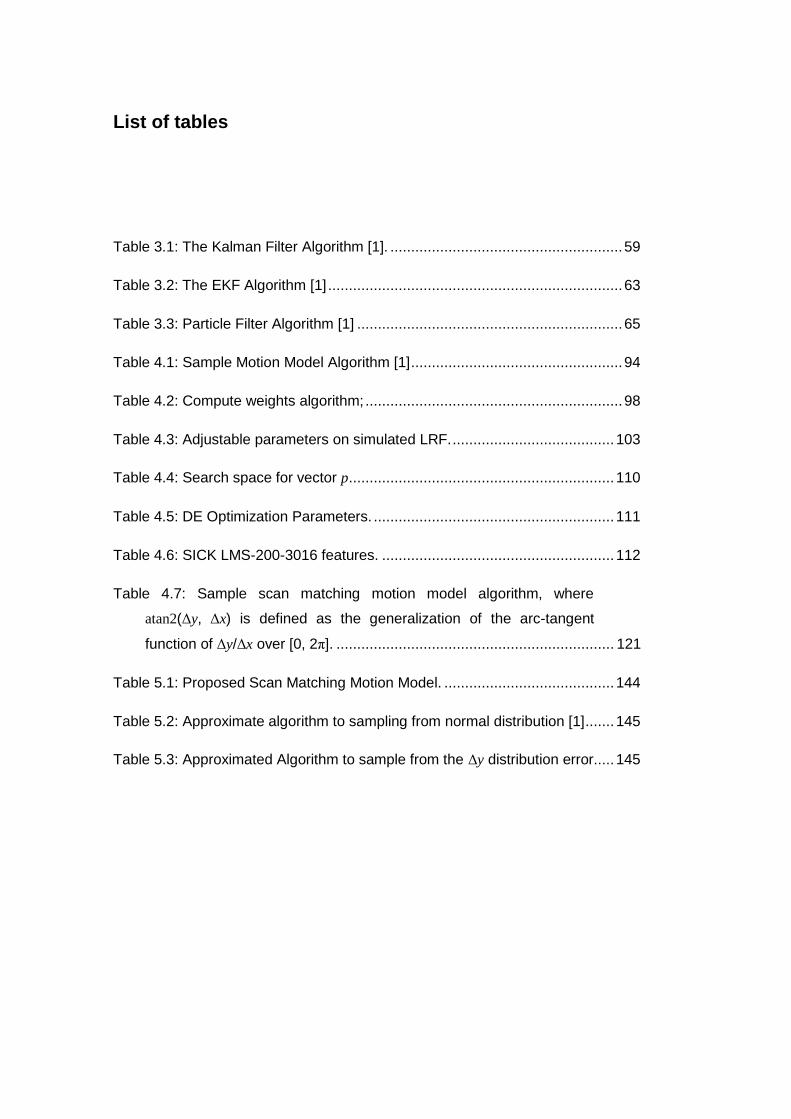
List of tables
Table 3.1: The Kalman Filter Algorithm [1]. ........................................................ 59
Table 3.2: The EKF Algorithm [1] ....................................................................... 63
Table 3.3: Particle Filter Algorithm [1] ................................................................ 65
Table 4.1: Sample Motion Model Algorithm [1] ................................................... 94
Table 4.2: Compute weights algorithm; .............................................................. 98
Table 4.3: Adjustable parameters on simulated LRF. ....................................... 103
Table 4.4: Search space for vector p ................................................................ 110
Table 4.5: DE Optimization Parameters. .......................................................... 111
Table 4.6: SICK LMS-200-3016 features. ........................................................ 112
Table 4.7: Sample scan matching motion model algorithm, where
atan2(Δy, Δx) is defined as the generalization of the arc-tangent
function of Δy/Δx over [0, 2π]. ................................................................... 121
Table 5.1: Proposed Scan Matching Motion Model. ......................................... 144
Table 5.2: Approximate algorithm to sampling from normal distribution [1] ....... 145
Table 5.3: Approximated Algorithm to sample from the Δy distribution error..... 145
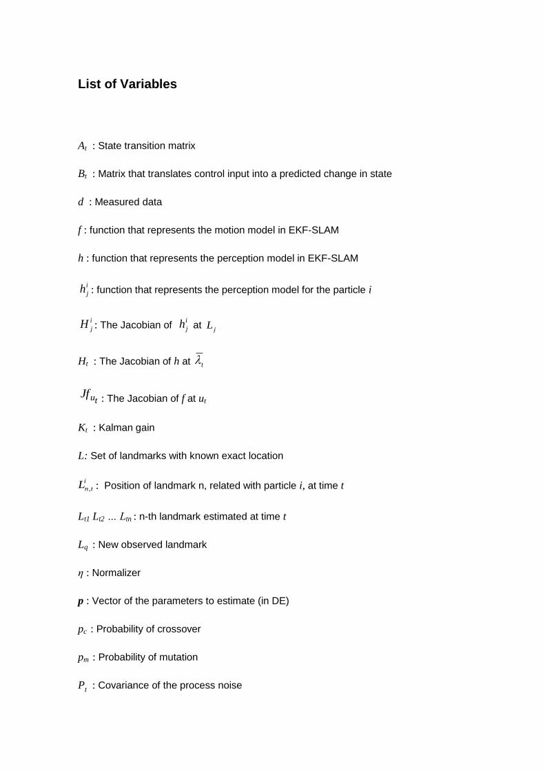
List of Variables
At : State transition matrix
Bt : Matrix that translates control input into a predicted change in state
d : Measured data
f : function that represents the motion model in EKF-SLAM
h : function that represents the perception model in EKF-SLAM
i
jh : function that represents the perception model for the particle i
i
jH : The Jacobian of i
jh at jL
Ht : The Jacobian of h at t
tuJf : The Jacobian of f at ut
Kt : Kalman gain
L: Set of landmarks with known exact location
i
tnL , : Position of landmark n, related with particle i, at time t
Lt1 Lt2 … Ltn : n-th landmark estimated at time t
Lq : New observed landmark
η : Normalizer
p : Vector of the parameters to estimate (in DE)
pc : Probability of crossover
pm : Probability of mutation
Pt : Covariance of the process noise
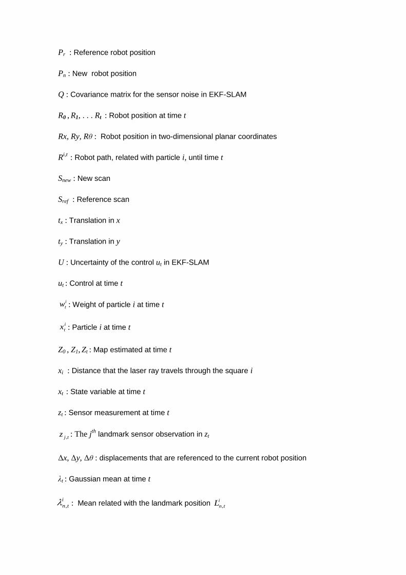
Pr : Reference robot position
Pn : New robot position
Q : Covariance matrix for the sensor noise in EKF-SLAM
R0 , R1, . . . Rt : Robot position at time t
Rx, Ry, Rθ : Robot position in two-dimensional planar coordinates
Ri,t
: Robot path, related with particle i, until time t
Snew : New scan
Sref : Reference scan
tx : Translation in x
ty : Translation in y
U : Uncertainty of the control ut in EKF-SLAM
ut : Control at time t
i
tw : Weight of particle i at time t
i
tx : Particle i at time t
Z0 , Z1, Zt : Map estimated at time t
xi : Distance that the laser ray travels through the square i
xt : State variable at time t
zt : Sensor measurement at time t
tjz , : The jth
landmark sensor observation in zt
Δx, Δy, Δθ : displacements that are referenced to the current robot position
λt : Gaussian mean at time t
i
tn, : Mean related with the landmark position i
tnL ,

ρi : Opacity of the square i
Σt : Gaussian covariance at time t
tt , : Predicted covariance and mean at time t
i
tn, : Covariance related with the landmark position i
tnL ,
ϕ : Rotation in z
Φt : Set of particles at time t

List of Abbreviations
SLAM : Simultaneous Localization and Mapping
LRF : Laser Range Finder
GPS: Global Positioning System
KF : Kalman Filter
PF : Particle Filter
EKF-SLAM : Extended Kalma Filter SLAM
FastSLAM : Fast SLAM
DP-SLAM : Distributed Particle SLAM
ICP : Iterative Closest Point
IDC : Iterative Dual Correspondence
ICL : Iterative Closest Line
HAYAI : The Highspeed and Yet Accurate Indoor/outdoor-tracking
NDT : Normal Distributed Transform
GA : Genetic Algorithm
GP : Genetic Programming
DE : Differential Evolution
LSLAM : Low SLAM
HSLAM: High SLAM
Stdv : Standard Deviation
19
20
1 Introduction and Problem Definition
1.1. Introduction
1.1.1. Robotics
“Robotics is the science of perceiving and manipulation the physical world
through computer-controlled mechanical devices” [1].
The word robot was first introduced in 1921 by the Czech novelist Karel
Čapek in his satirical drama entitled: Rossum´s Universal Robots. It is derived
from the Czech word robota, which literally means “forced laborer” or “slave
laborer” [2]. From there this word was popularized by science fiction, assigning it
to machines with anthropomorphic characteristics, fitted with action and decision
capabilities, similar or higher than humans [3]. Examples of successful robotics
system include mobile platforms for planetary exploration, robotics arms in
assembly lines, cars traveling autonomously on highways, actuated arms that
assist surgeons and so on.
Mobile robot systems operate in increasingly unstructured environments,
inherently unpredictable. “As a result, robotics is moving into areas where sensor
input becomes increasingly important, and where robot software has to be robust
enough to cope with a range of situations – often too many to anticipate them all”
[1]. Robotics is becoming a software science, where the target is to develop sturdy
software that enables robots to overcome the numerous challenges in unstructured
and dynamic environments.
21
1.1.2. Uncertainty in Robotics
Uncertainty in robotics arises from five different factors [1]:
1. Environment. Environments such as private homes and highways are
highly dynamic and unpredictable
2. Sensors. Limitation in sensors arises from their range and resolution. In
addition, sensors are subject to noise.
3. Robots. “Robot actuation involves motors that are, at least to some
extent, unpredictable, due to effects such as control noise and wear-and-
tear” [1].
4. Models. Models are idealization of the real world. They only partially
model the physical processes of the robot and its environment.
5. Computation. “Robots are real-time systems, which limits the amount
of computation that can be carried out” [1]. Many algorithms are
approximate, reaching timely response through slaughtering accuracy.
“Traditionally such uncertainty has mostly been ignored in Robotics” [1].
However, as robots are moving away into increasingly unstructured environments,
the ability to deal with uncertainty is crucial for building successful systems.
1.2. Problem Definition
The scope of this work is related to the SLAM problem. SLAM
(Simultaneous Localization and Mapping) is one of the most widely researched
subfields of robotics, in special in mobile robotic systems.
Let’s consider a mobile robot which is using wheels connected to a motor,
actuators and a camera. Consider that the robot is manipulated by an operator
mapping inaccessible places. The actuators allow the robot to move around, and
the camera provides visual information for the operator to know where objects are
22
and how the robot is oriented in reference to them. What the human operator is
doing is an example of SLAM.
“Thus, the SLAM subfield of Robotics attempts to provide a way for robots
to perform SLAM autonomously. A solution to the SLAM problem would allow a
robot to make maps without any human assistance whatsoever” [4].
In the following, the SLAM idea is graphically presented (example taken
from [4]).
1.2.1. Localization overview
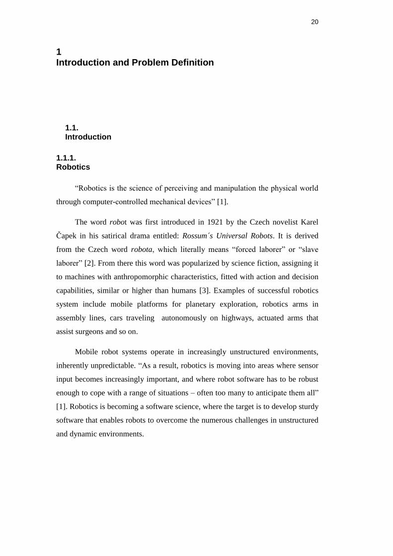
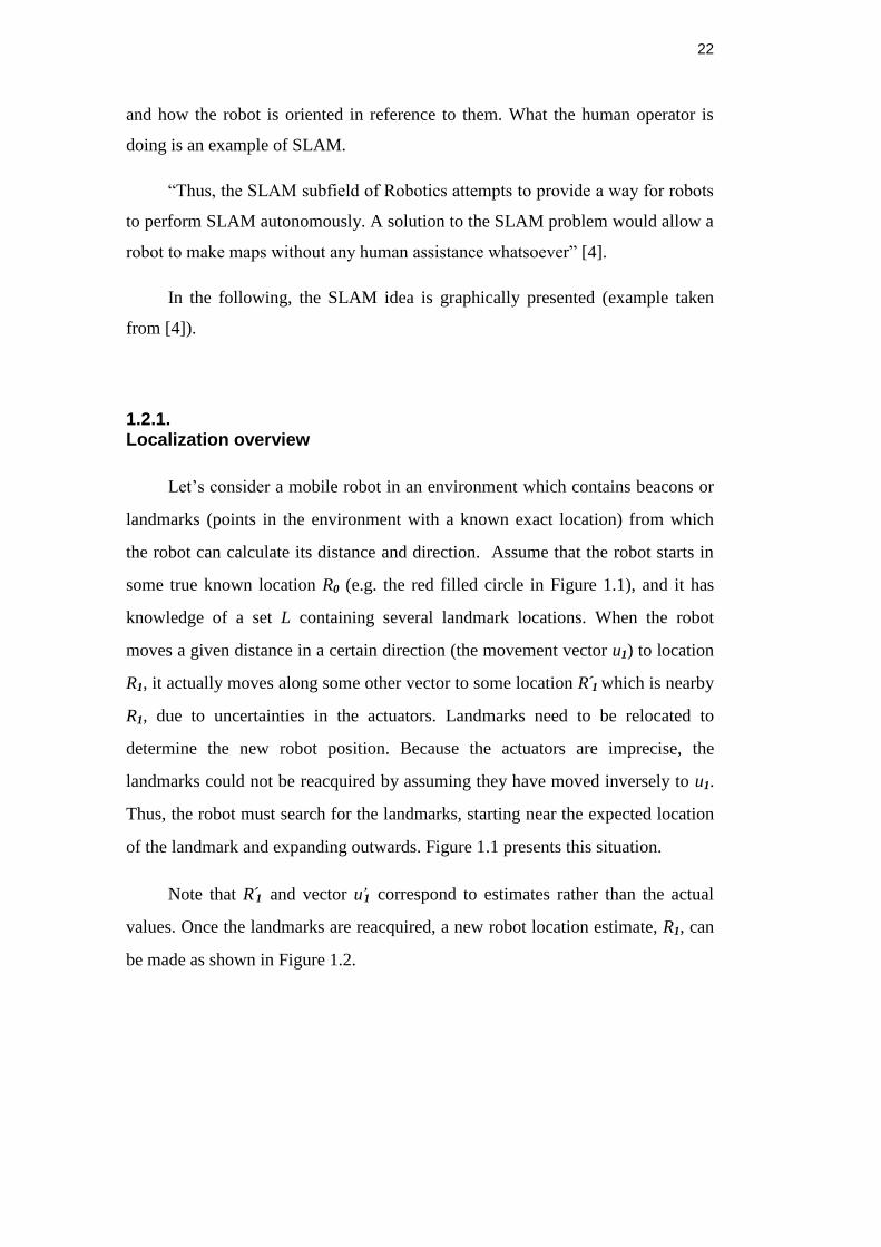
Let’s consider a mobile robot in an environment which contains beacons or
landmarks (points in the environment with a known exact location) from which
the robot can calculate its distance and direction. Assume that the robot starts in
some true known location R0 (e.g. the red filled circle in Figure 1.1), and it has
knowledge of a set L containing several landmark locations. When the robot
moves a given distance in a certain direction (the movement vector u1) to location
R1, it actually moves along some other vector to some location R 1 which is nearby
R1, due to uncertainties in the actuators. Landmarks need to be relocated to
determine the new robot position. Because the actuators are imprecise, the
landmarks could not be reacquired by assuming they have moved inversely to u1.
Thus, the robot must search for the landmarks, starting near the expected location
of the landmark and expanding outwards. Figure 1.1 presents this situation.
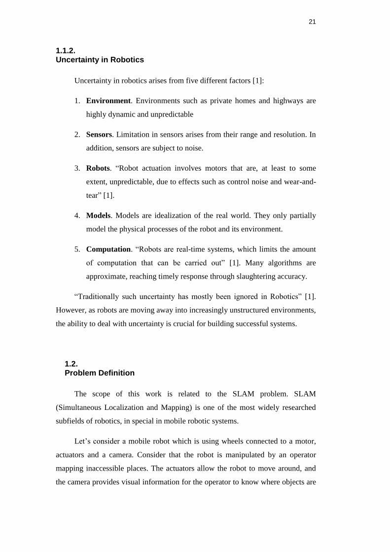
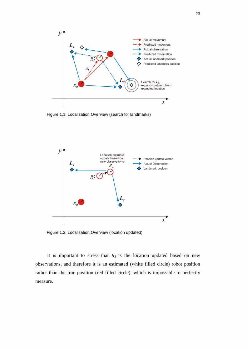
Note that R 1 and vector u’1 correspond to estimates rather than the actual
values. Once the landmarks are reacquired, a new robot location estimate, R1, can
be made as shown in Figure 1.2.
23
Figure 1.1: Localization Overview (search for landmarks)
Figure 1.2: Localization Overview (location updated)
It is important to stress that R1 is the location updated based on new
observations, and therefore it is an estimated (white filled circle) robot position
rather than the true position (red filled circle), which is impossible to perfectly
measure.
24
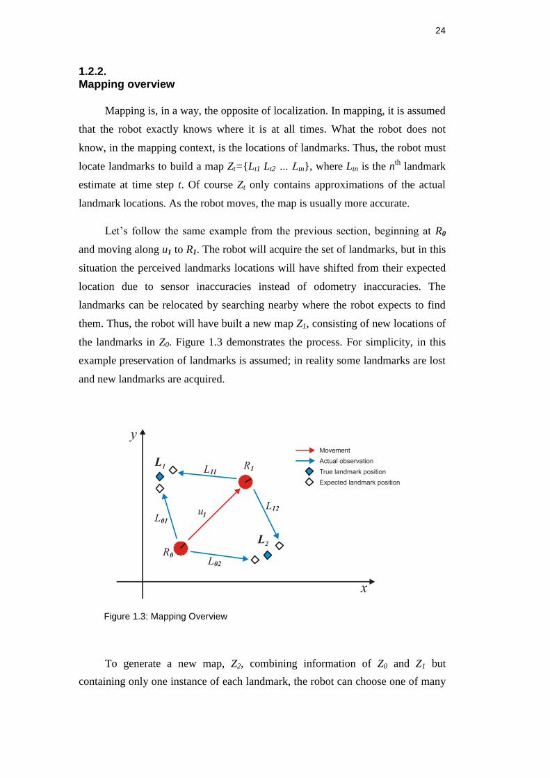
1.2.2. Mapping overview
Mapping is, in a way, the opposite of localization. In mapping, it is assumed
that the robot exactly knows where it is at all times. What the robot does not
know, in the mapping context, is the locations of landmarks. Thus, the robot must
locate landmarks to build a map Zt={Lt1 Lt2 … Ltn}, where Ltn is the nth
landmark
estimate at time step t. Of course Zt only contains approximations of the actual
landmark locations. As the robot moves, the map is usually more accurate.
Let’s follow the same example from the previous section, beginning at R0
and moving along u1 to R1. The robot will acquire the set of landmarks, but in this
situation the perceived landmarks locations will have shifted from their expected
location due to sensor inaccuracies instead of odometry inaccuracies. The
landmarks can be relocated by searching nearby where the robot expects to find
them. Thus, the robot will have built a new map Z1, consisting of new locations of
the landmarks in Z0. Figure 1.3 demonstrates the process. For simplicity, in this
example preservation of landmarks is assumed; in reality some landmarks are lost
and new landmarks are acquired.
Figure 1.3: Mapping Overview
To generate a new map, Z2, combining information of Z0 and Z1 but
containing only one instance of each landmark, the robot can choose one of many
25
options. For example, it can choose any point on the line connecting L0n and L1n
(note that L0n and L1n are two conflicting perceived locations of landmark n).
Whichever the method selected for incorporating new sensor readings, it
seems safe to assume that Zt will improve as time t increases.
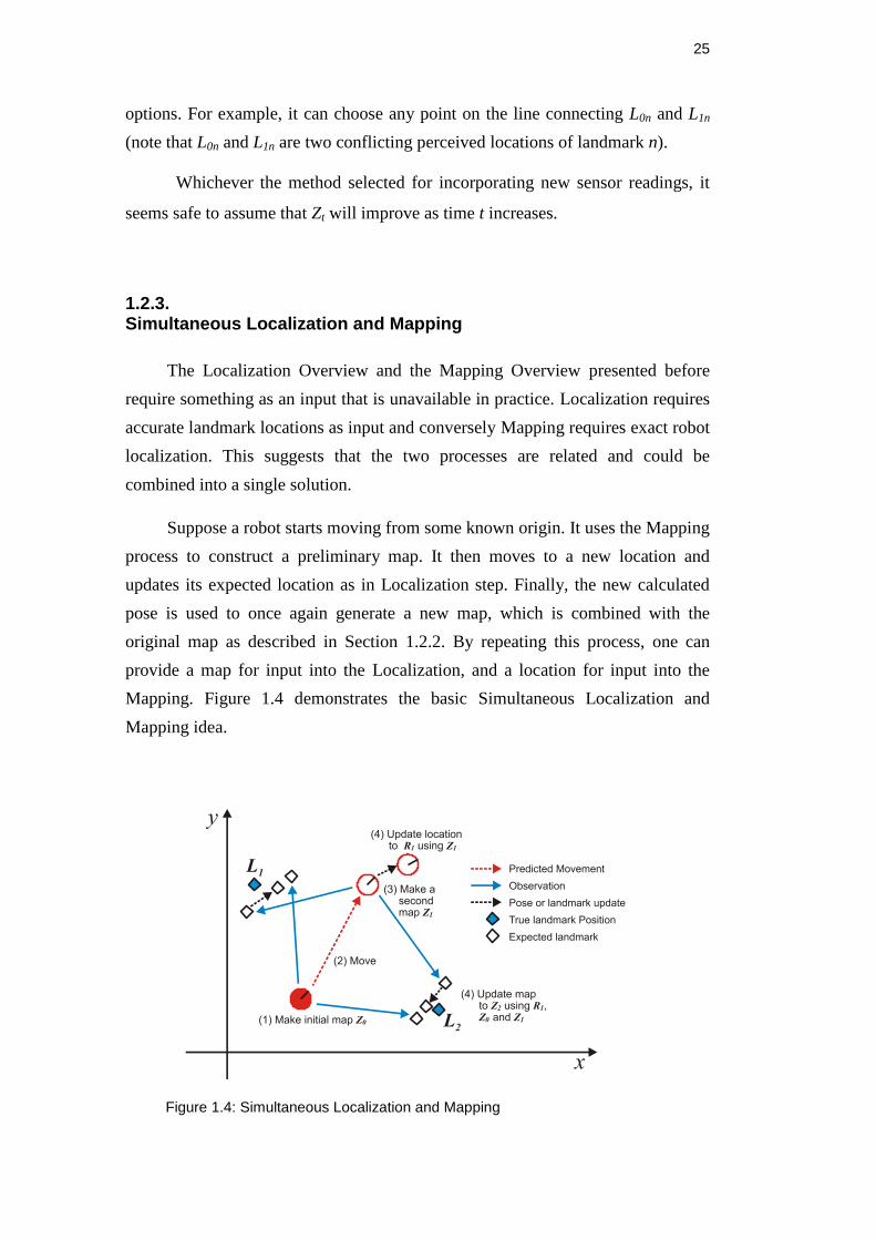
1.2.3. Simultaneous Localization and Mapping
The Localization Overview and the Mapping Overview presented before
require something as an input that is unavailable in practice. Localization requires
accurate landmark locations as input and conversely Mapping requires exact robot
localization. This suggests that the two processes are related and could be
combined into a single solution.
Suppose a robot starts moving from some known origin. It uses the Mapping
process to construct a preliminary map. It then moves to a new location and
updates its expected location as in Localization step. Finally, the new calculated
pose is used to once again generate a new map, which is combined with the
original map as described in Section 1.2.2. By repeating this process, one can
provide a map for input into the Localization, and a location for input into the
Mapping. Figure 1.4 demonstrates the basic Simultaneous Localization and
Mapping idea.
Figure 1.4: Simultaneous Localization and Mapping
26
One thing to notice with this combined localization and mapping algorithm
is that one does not provide completely accurate input to either the mapping or the
localization components.
1.3. Motivation
Petrobras operates in oil and gas exploitation at Amazon, in the province of
Urucu (AM), at the Solimões River, about 650 km from Manaus City. To drain
this production, it has been built two gas pipelines: Coari-Manaus and Urucu
Porto Velho, with 420 Km of extension from Manaus as well.
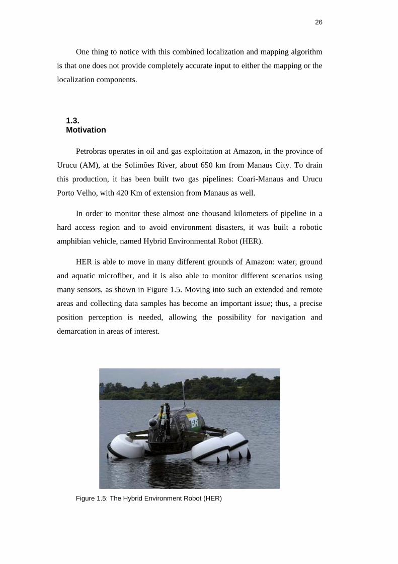
In order to monitor these almost one thousand kilometers of pipeline in a
hard access region and to avoid environment disasters, it was built a robotic
amphibian vehicle, named Hybrid Environmental Robot (HER).
HER is able to move in many different grounds of Amazon: water, ground
and aquatic microfiber, and it is also able to monitor different scenarios using
many sensors, as shown in Figure 1.5. Moving into such an extended and remote
areas and collecting data samples has become an important issue; thus, a precise
position perception is needed, allowing the possibility for navigation and
demarcation in areas of interest.
Figure 1.5: The Hybrid Environment Robot (HER)
27
HER acquires its position using a GPS system. However, it is prone to
failure because of obstructions in satellite signal, caused by local vegetation. In
this case, HER needs to acquire its position in a different way, in order to continue
its mission or to search places with better satellite reception. The use of odometers
is not a good choice due to frequent slipping on the ground; beyond, it does not
have any utility over water. Localization by cameras also does not presents good
results due to high similarity between vegetation images, making hard a reliable
keypoints establishment. Inertial platforms would help in the localization of the
robot, but would not have any utility to detect obstacles.
So, the use of a Laser Range Finder (LFR) represents great advantages,
cause it is able, not only to locate the robot or mapping the environment, but also
to detect obstacles on the robot´s path.
1.4. Objective
The objective of this work is to perform SLAM with limited sensor
capabilities. More specifically, it is shown that localization and mapping can be
performed without odometry measurements, just by using a single Laser Range
Finder (LRF).
To accomplish that, first a detailed explanation of SLAM algorithms
implementations is given, focusing on the: EKF-SLAM, FastSLAM, and DP-
SLAM methods. Then, a Genetic Algorithm is implemented for Normal
Distribution Transform (NDT) optimization, in order to obtain robot displacement
without odometry information. An implementation for 3D mapping is shown,
using DP-SLAM, which does not use predetermined landmarks (not dealing either
with data association problems). Finally a virtual 3D environment is simulated
including virtual Laser Range Finder (LRF) readings, to validate the presented
methodology. Experimental data from actual LRF readings are also used to
evaluate the performance of the algorithms.
28
1.5. Organization of the Thesis
This thesis is divided into six chapters, described as follows:
Chapter 2 comprises the theory necessary for Probabilistic Robotic. The
basic concepts of representing uncertainties in a planar robot environment are
shown. Also the main algorithms for scan matching are given, emphasizing on the
Normal Distribution Transform(NDT). Concluding with Genetic Algorithms and
Differential Evolution (DE).
Chapter 3 describes the principal algorithms for the SLAM solutions,
including EKF-SLAM, FastSLAM and DP-SLAM. Besides, is presented a review
for 3D SLAM solutions and 3D mapping.
Chapter 4 gives a detailed implementation of the principal SLAM solutions:
EKF-SLAM, FastSLAM and DP-SLAM. Is explained also, the simulated Laser
Range Finder (RLF) in a structured environment, developed for testing the
proposed methods. In addition, is explained the NDT optimization using
Differential Evolution, in order to get robot displacements without odometry
information.
Chapter 5 presents the results obtained in simulated and real data acquired
from the literature.
Chapter 6 presents comments and conclusions to the performed work.
29
2. Theoretical Basis
2.1. Probabilistic Robotics
“The key idea of Probabilistic Robotics is to represent uncertainty explicitly,
using the calculus of probability theory” [1]. In other words, instead of relying on
a single “best guess” probabilistic algorithms represent information by
probabilistic distributions. By doing so, probabilistic robotics can mathematically
represent ambiguity and degree of belief, enabling them to accommodate all
sources of uncertainty.
The advantage of probabilistically programming robots, compared to other
approaches that do not explicitly represent uncertainty, is simply because:
“A robot that carries a notion of its own uncertainty and that acts
accordingly is superior to one that does not.” [1].
Probabilistic approaches are typically more robust under sensor limitation,
sensor noise, environment dynamics, and so on. They are well suited to complex
and unstructured environments, where the ability to deal with uncertainty is quite
important. “Probabilistic algorithms are broadly applicable to virtually every
problem involving perception and action in the real world” [1].
All these advantages, however, come at a price. The two most cited
limitations of probabilistic algorithms are: a need to approximate and
computational inefficiency. Because probabilistic algorithms consider entire
probability densities, they are less efficient than non-probabilistic ones.
Computing exact posterior distributions is typically infeasible, since distributions
over the continuum possess infinitely many dimensions (most robot worlds are
continuous). Sometimes, uncertainty can be approximated with a compact
parametric model (e.g. discrete distributions or Gaussians); in other cases, a more
complicated representations most be employed.
30
“At the core of probabilistic robotics is the idea of estimating state from
sensor data” [1]. This sensor data are not directly observable, but that can be
inferred. A robot has to rely on its sensors to gather information, while this
information is only partial, and corrupted by noise. Thus, state estimation seeks to
recover state variables from data.
2.1.1. Bayes Filter and SLAM
In Probabilistic Robotics, all quantities related in estimation such as sensor
measurements, controls, state of the robot and its environment might be modeled
as random variables. Random variables can take on multiple values, and they
behave according to probabilistic laws. Probabilistic inference is the process of
calculating these laws.
“Bayes rule is the archetype of probabilistic inference” [5]. It plays a
predominant role in probabilistic robotics. Therefore, it is the basic principle
underlying virtually every single successful SLAM algorithm. The Bayes rule is
stated as [1]:
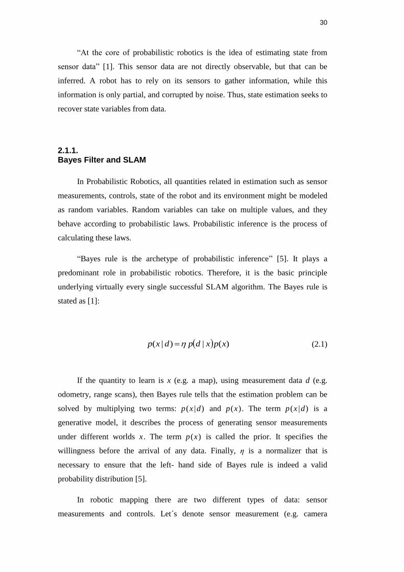
)(|)|( xpxdpdxp (2.1)
If the quantity to learn is x (e.g. a map), using measurement data d (e.g.
odometry, range scans), then Bayes rule tells that the estimation problem can be
solved by multiplying two terms: p(x|d) and p(x). The term p(x|d) is a
generative model, it describes the process of generating sensor measurements
under different worlds x . The term p(x) is called the prior. It specifies the
willingness before the arrival of any data. Finally, η is a normalizer that is
necessary to ensure that the left- hand side of Bayes rule is indeed a valid
probability distribution [5].
In robotic mapping there are two different types of data: sensor
measurements and controls. Let´s denote sensor measurement (e.g. camera
31
images, LRF scans) by the variable z, and the control (e.g. motion command,
odometry) by u. Let us assume that the data is collected in alternation:
...,,,, 2211 uzuz (2.2)
where subscripts are used as time index.
“In the field of robot mapping, the single dominating scheme for integrating
such temporal data is known as Bayes Filter” [5].
The Bayes Filter is the extension of Bayes rule to temporal estimation
problems[5]. It is a recursive estimator to compute posterior probability
distributions over quantities that cannot be observed directly – such as a map or
robot position. Let’s call this unknown quantity the state xt, where t is the time
index. The generic Bayes filter calculates a posterior probability over the state xt
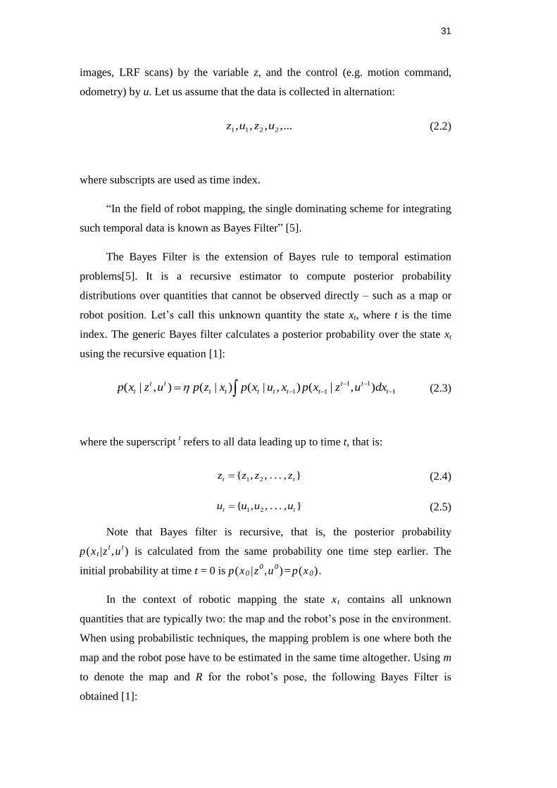
using the recursive equation [1]:
1
11
11 ),|(),|()|(),|( t
tt
tttttt
tt
t dxuzxpxuxpxzpuzxp (2.3)
where the superscript t refers to all data leading up to time t, that is:
},...,,{ 21 tt zzzz (2.4)
},...,,{ 21 tt uuuu (2.5)
Note that Bayes filter is recursive, that is, the posterior probability
p(x t |zt,u
t) is calculated from the same probability one time step earlier. The
initial probability at time t = 0 is p(x0 |z0,u
0) = p(x0).
In the context of robotic mapping the state x t contains all unknown
quantities that are typically two: the map and the robot’s pose in the environment.
When using probabilistic techniques, the mapping problem is one where both the
map and the robot pose have to be estimated in the same time altogether. Using m
to denote the map and R for the robot’s pose, the following Bayes Filter is
obtained [1]:
32
),|,( tt
tt uzmp R
11
11
1111 ),|,(),,|,(),|( tt
tt
tttttttttt dmduzmpmumpmzp RRRRR
(2.6)
If assumed a static world, the time index can be omitted when referring to
the map m. Also, most approaches assume that the robot motion is independent of
the map. And finally, using the Markov assumption, which postulates that past
and future data are independent if one knows the current state xt, the state xt can be
estimated using only the state xt-1 one step earlier. This results in a convenient
form of the Bayes Filter for the robot mapping problem [5]:
),|,( tt
t uzmp R
1
11
11 ),|,(),|(),|( t
tt
tttttt RRRRR duzmpupmzp
(2.7)
This estimator does not require integration over maps m, as it was the case
for the previous one from eq. (2.6). The static world assumption is quite
important, because such integration is difficult due to the high dimensionality of
the space of all maps.
In eq. (2.7) two distributions probabilities have to be specified: p(Rt|ut, Rt-1)
and p(zt|Rt,m). Both are generative models of the robot and its environment.
The probability distribution p(Rt|ut, Rt-1), often called to as motion model,
specifies the effect of the control u on the state. It describes the probability that
the control u, if executed at the world state Rt-1, leads to the state Rt.
The probability p(zt|Rt,m), often called to as perception model, describes in
probabilistic terms how sensor measurements z are generated for different poses
Rt and maps m.
However, eq. (2.7) cannot be implemented on a digital computer in its
general stated form. This is because the posterior over the space of all maps and
robot poses is a probability distribution over a continuous space, hence possesses
infinitely many dimensions. Therefore, any working mapping algorithm has to
take additional assumptions. These assumptions and their implications on the
33
resulting algorithms and maps constitute the main differences between the
different solutions to the SLAM.
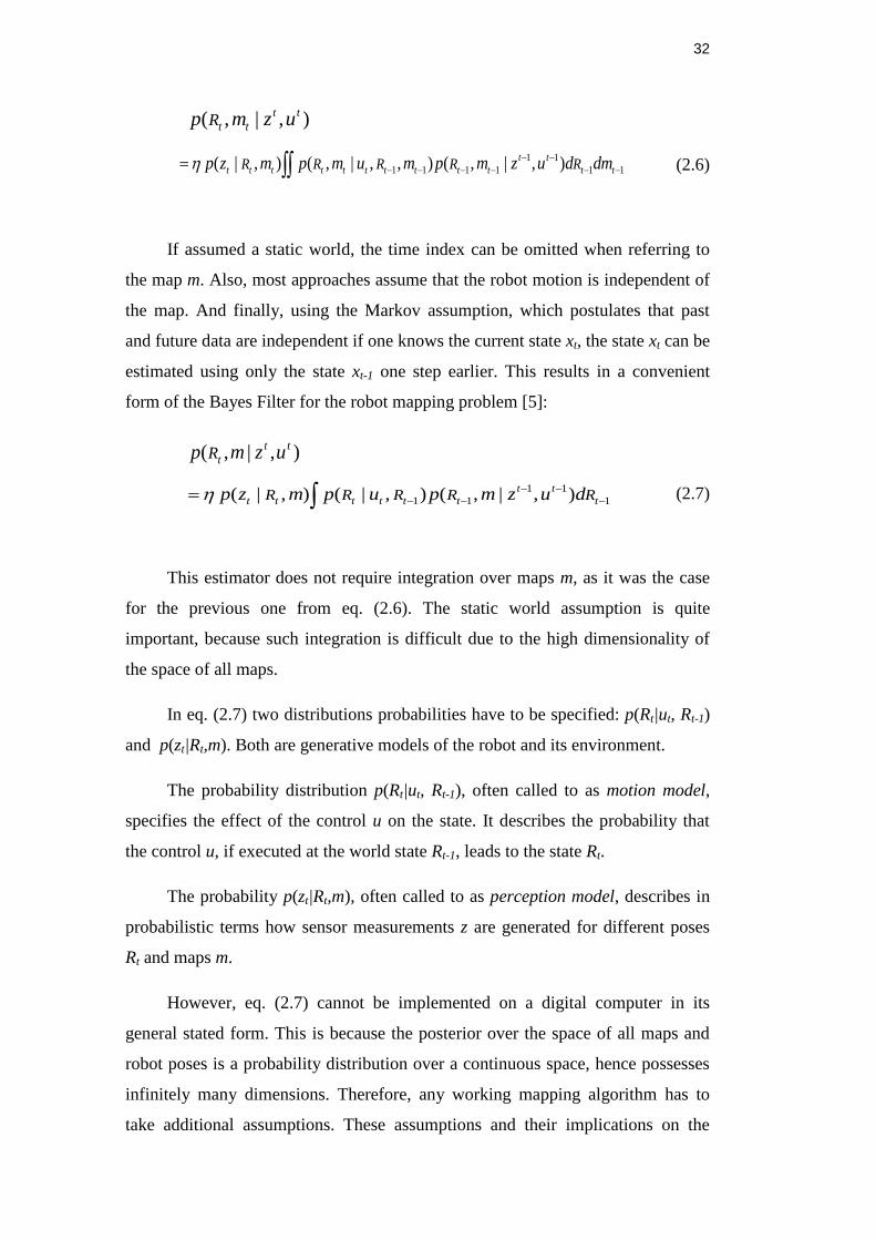
Figure 2.1 shows a generative probabilistic model (dynamic Bayes network)
that underlies the essential of SLAM.
Figure 2.1: SLAM like a Dynamic Bayes Network
In particular, the robot poses, denoted by R1, R2, …, Rt, evolve over time as
a function of the controls, denoted by u1, u2, …, ut. The map is composed (as it
will be seen later) by landmarks and each measurement of them, denoted by z1, z2,
…, zt, which are a function of its position L1, L2, …, Ln and of the robot pose at the
time the measurement was taken.
Note that in this SLAM equation analysis the odometery ut is assumed to be
known, and this assumption will be kept till the Section 4.5.1 where odometry is
replaced by Scan Matching.
2.1.2. Motion Model
“Robot motion models play an important role in modern robotics
algorithms” [6]. The main purpose of a motion model is to model the relationship
between a control input to the robot and a change in the robot´s configuration,
34
pose and map. Good models will capture not only systematic errors, but it will
also capture the stochastic nature of the motion. The same control input will
almost never produce the same result. “Thus, the effects of a robot’s action are,
therefore, best described as distributions” [6].
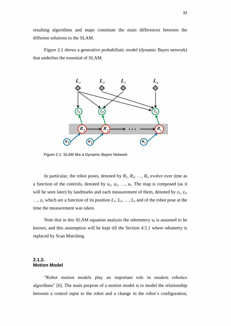
This thesis focuses entirely on kinematics for mobile robots operating in
planar environments. Kinematics describes the effect of control actions on the
configuration of a robot. A rigid mobile robot is commonly described by six
variables, its three-dimensional Cartesian coordinates and its three Euler angles
(roll, pitch, yaw) referred to an external coordinate frame. But in a planar
environment, the position of a mobile robot is summarized by three variables: its
two-dimensional planar coordinates referred to an external coordinate frame,
along with its angular orientation.
R
Ry
Rx
R
(2.8)
Figure 2.2 illustrates a robot pose in a plane.
Figure 2.2: Robot pose
The orientation of a robot is often called bearing, or heading direction.
35
The probabilistic kinematic model, or motion model, plays the role of the
state transition model in Mobile Robotics. As described in the previous section,
this model is the probability distribution:
),|( 1ttt RR up
(2.9)
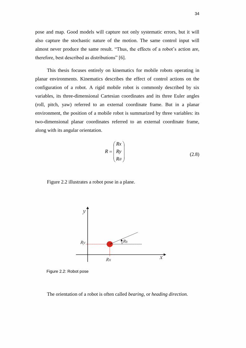
Figure 2.3 shows two examples that illustrate the motion model for a rigid
mobile robot in a planar environment. The robot’s initial pose, in both cases, is
Rt-1. The distribution p(Rt|ut, Rt-1) is visualized in the form of a gray shaded area:
darker areas mean more probability in robot position. In both figures, the robot
moves forward some distance, during which it may accumulate translational and
rotational errors. The right figure shows a larger spread of uncertainty due to a
more complicated motion.
Figure 2.3: The motion model, showing posterior distributions of the robot’s pose
after executing the motion command ut (red striped line). The darker a location, the
more likely it is.
There are two motion models usually used. “The first model assumes that
the motion data ut specifies the velocity commands given to the robot’s motors”
[1]. Many commercial mobile robots (e.g. differential drive, synchro drive) are
actuated by independent translational and rotational velocities. The second model,
which is used in this work, assumes that ut contains odometry information
(distance traveled, angle turned).
36
However, odometry is only available as the robot moves. Hence it cannot be
used for motion planning, such as collision avoidance [1]. “Technically, odometry
are sensor measurements, not controls” [1]. But it is common to simply consider
odometry as if it was a control input signal.
2.1.3. Perception Model
“The perception model comprises the second domain-specific model in
probabilistic robotics, next to the motion model” [1]. In probabilistic terms, the
Perception Model describes how sensor measurements z are generated for
different poses R and maps m. As described before, this is modeled by:
),|( mRzp tt (2.10)
The Perception Model account for the uncertainty in the robot’s sensors.
Thus, it explicitly models noise in sensor measurement. It could say that better
results are acquired by a more accurate Perception Model. However, it is almost
impossible to accurately model a sensor; reference [1] gives two primarily
reasons[1]: “First, developing an accurate perception model can be extremely
time-consuming; and second, an accurate model may require state variables that
are not known, such as the surface material” [1]. In this way Probabilistic
Robotics, instead of modeling the Perception Model by a deterministic function
z=f(x), accommodates the inaccuracies of Perception Model by a conditional
probability density, p(z|x). “Herein lies a key advantage of probabilistic
techniques over classical robotics” [1].
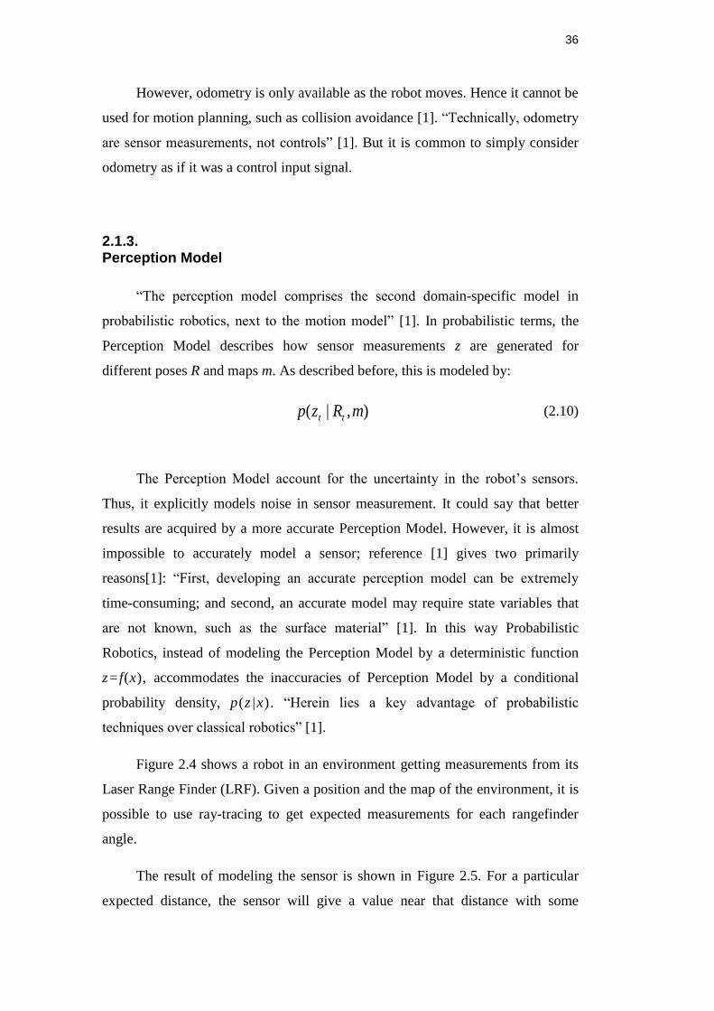
Figure 2.4 shows a robot in an environment getting measurements from its
Laser Range Finder (LRF). Given a position and the map of the environment, it is
possible to use ray-tracing to get expected measurements for each rangefinder
angle.
The result of modeling the sensor is shown in Figure 2.5. For a particular
expected distance, the sensor will give a value near that distance with some
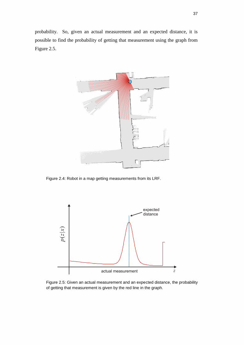
37
probability. So, given an actual measurement and an expected distance, it is
possible to find the probability of getting that measurement using the graph from
Figure 2.5.
Figure 2.4: Robot in a map getting measurements from its LRF.
Figure 2.5: Given an actual measurement and an expected distance, the probability
of getting that measurement is given by the red line in the graph.
38
Today’s robots use a variety of sensor types, such as tactile sensors, range
finder sensors, sonar sensors or cameras. The model specifications depend on the
sensor type.
2.2. Map Representation
There are many reasons to have a representation of the robot’s environment.
Some of the purposes of having a map are listed in the following:
Localization. The robot localization is possible making a correspondence
between a given map and the observation of the robot’s environment.
Motion planning. Once the robot is located and given a target position, all
necessary movements in the map can be compute to successfully move to the
target.
Collision avoidance. Using a map and robot’s localization the navigation is
possible without collisions.
Human use. The map constructed by the robot can be used for exploration
tasks in potentially hazardous environments.
In general, the map representation can be grouped into three main types:
Geometric, Topological and Hybrid. However the general tendency in SLAM is to
use geometric representation. Thus, this representation has also a subdivision:
Landmark (or feature maps) and Grid maps.
2.2.1. Landmark Maps
The landmark-based maps consist of a set of distinctive point localizations
that are referred to a global reference system. In structured domains such as
indoor environments, landmarks are usually modeled as geometric primitives such
as points, lines or surfaces.
39
The main advantage of landmark-base maps is their representation
compactness. By contrast, this kind of map requires the existence of structures or
objects that are distinguishable enough from each other. Thus, an extra algorithm
for recognizable and repeatedly detectable landmark extraction is needed.
In practice, good landmarks may have similar traits, which often make them
difficult to distinguish from each other. When this happens the problem of data
association, also known as the correspondence problem, has to be addressed. “The
correspondence problem is the problem of determining if sensor measurements
taken at different points in time correspond to the same physical object in the
world” [5]. It is a difficult problem, because the number of possible hypotheses
can grow exponentially.
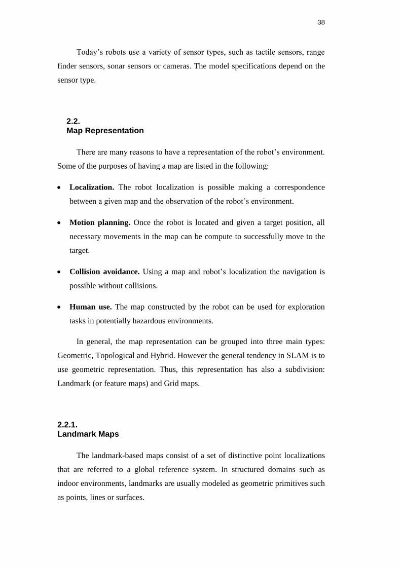
Figure 2.6 shows a simulated landmark-based map, where the blue asterisks
represent the landmarks and the small triangle the robot position.
Figure 2.6: Simulated Landmark Map
40
2.2.2. Grid Maps
A grid map, or occupancy grid, is a popular and intuitive method to describe
an environment. Occupancy grids were originally developed at Carnegie Mellon
University in 1983 for sonar navigation within a lab [7].
Occupancy grids divide the environment up into a regular grid square, all of
equal size. “Each of these grid squares correspond to a physical area in the
environment and, as such, each square contains a different set of objects or
portions of an object” [6]. An occupancy grid is an ideal representation of the
environment, containing information on whether a square in the real environment
is occupied or not.
The occupancy grid representation can be generalized into two types:
deterministic and stochastic [6], described as follows.
Deterministic map grids are the simplest representation, having two values for
each grid square. Typically squares are considered as either Empty or
Occupied, also sometimes is include a value for Unknown (or Unobserved).
However, this representation is an exaggerated simplification for the sensors,
since almost never a sensor will see a square of the environment which is both
completely occupied and accurately observed.
Stochastic maps, besides of Occupied and Empty, have a gradual scale of
various degrees of occupancy. What percentage of the square is believed to be
occupied, or how transparent the object is to the sensor are some factors that
affect the occupancy value. The stochastic representation and the
corresponding observation model need to be properly tuned for the sensor
used.
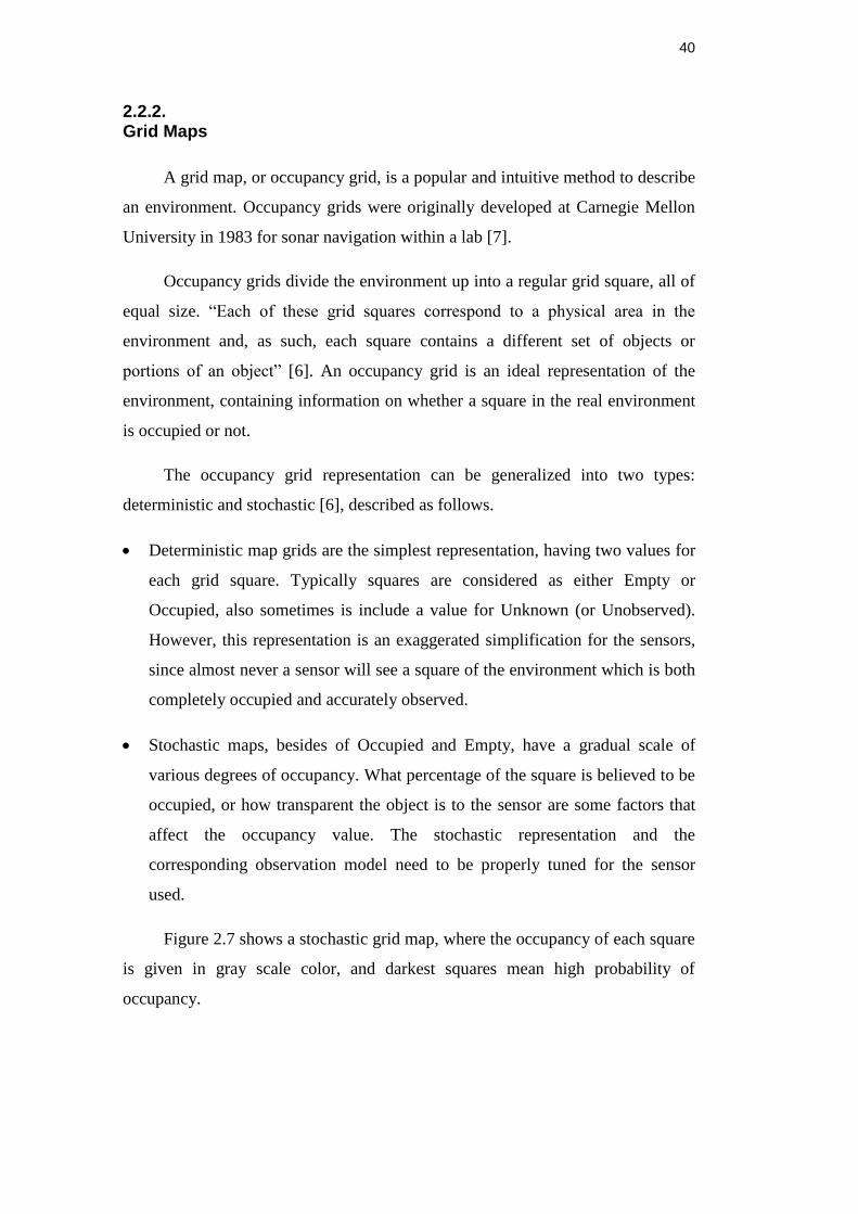
Figure 2.7 shows a stochastic grid map, where the occupancy of each square
is given in gray scale color, and darkest squares mean high probability of
occupancy.
41
Figure 2.7: Grid Map: White regions mean unknown areas, light gray represents
unoccupied areas, and darker gray to black represent increasingly occupied areas.
This work uses occupancy grid maps for environment representation,
specifically stochastic occupancy grid maps.
2.3. Scan Matching
“Many SLAM algorithms are based on the ability to match two range scans
or to match a range scan to a map” [8]. Laser Range Fiders (LRF) are popular
sensors to get the input for scan matching, since their high reliability and their low
noise in many situations.
The goal of scan matching is to find the relative displacement between the
two positions at which the scans were taken. If a robot starts at position Pr (which
is a reference pose), takes a scan Sr (reference scan), after that it moves through a
static environment to a new pose Pn and takes another scan Sn (new scan), then
scan matching seeks the difference of position Pn from posistion Pr (the relative
translation and rotation) by aligning the two scans.
42
“The basis of most successful algorithms is the establishment of
correspondences between primitives of the two scans” [8], i.e. point-to-point or
feature-to-feature.
Different routines are developed to use point-to-point matching approaches
such as the Iterative Closest Point (ICP) and the Iterative Dual Correspondence
(IDC), both proposed by Lu and Milios [9]; and another, The Iterative Closest
Line (ICL) proposed by Alshawa [10].
In [11] it is proposed a method that searches for features like corners and
jump-edges from raw range scans. Another method based on feature extraction is
HAYAI proposed in [12]. This method solves the self-localization problem for
high speed robots.
One method that does not use correspondences between scans is the Normal
Distribution Transform proposed in [8]. This method transforms the discrete set
of 2D points reconstructed from a single scan into a piecewise continuous
differentiable probability density defined on the 2D plane.
This work uses the NDT for scan matching but without using odometry
information. But before getting to it; let’s briefly review some of methods used for
scan matching including NTD.
2.3.1. Point to Point Correspondence Methods.
The Iterative Closest Point (ICP)
The most general matching point to point approach was introduced
by Lu and Milios in [9]. This is essentially a variant of the ICP (Iterative
Closest Point) algorithm applied to laser scan matching.
A scan is a sequence of points which represent a 2D plane contour of
the local environment. “Due to the existence of random sensing noise and
self-occlusion, it may be impossible to align two scans perfectly” [9]. Thus
this method assumes two types of discrepancies between scans:
43
o in the first type, there are small deviations of scan points from the true
contour due to random sensing noise, and
o the other type of discrepancy is the gross difference between the scans
caused by occlusion. These discrepancy types are called outliers.
Adopting these criterions, ICP finds the best alignment of the
overlapping part in the sense of minimum least-square errors, while
ignoring the outlier parts. That is way ICP also need of correspondence
search and outlier detection algorithms.
Lu and Milios [9] present two scan matching methods based on ICP.
The first considers the two components (rotational and translational)
separately; alternately fixing one, then optimizing the other. Given the
rotation, least-square optimization is used to acquire translation.
Their second method called Iterative Dual Correspondence (IDC)
combines two ICP-like algorithms with different point-matching
heuristics.
The Iterative Closest Line (ICL)
“ICL is similar to ICP, except that instead of matching query points
to reference points, the query points are matched to lines extracted from
the reference points” [13].
2.3.2. Feature to Feature Correspondence Methods.
Feature Based Laser Scan Matching for Accurate and high speed
Mobile Robot Localization.
Proposed by Aghamohammadi et al. [11]. This method divides the
features into two types: features corresponding to the jump-edges and
those corresponding to the corners detected in the scan.
In order to detect jump-edges, this method uses the natural
consecutive order of points in the scan. Thus it defines a dth which is the
44
maximum distance between two consecutive scan points. Beyond dth these
two consecutive points can be considered as jump-edges.
To obtain the second class of features, the corners, this method uses
a line fitting algorithm. Thus the split-and-merge algorithm is used but
only for line fitting. In this way, using two points taken of two consecutive
lines, it searches for the farthest point to the straight line joining these two
points.
Finally, after extracting features for two consecutive scans, a
matching algorithm, based on a dissimilarity function is calculated.
This method is fast and it can be used for high speed mobile robot,
but it suffers when the environment does not have corners or when it has
circular walls, because no corners could be extracted and false jump-edges
could be acquired.
The Highspeed and Yet Accurate Indoor/outdoor-tracking (HAYAI)
HAYAI was proposed by Lingemann et al. [12]. This uses the
inherent order of the scan data, allowing the application of linear filters for
fast reliable feature detection.
Thus, this method chooses extrema in the polar representation of a
scan as natural features. These extrema correlate to corners and jump-
edges in Cartesian space. The usage of polar coordinates implicates a
reduction by one dimension, since all operations deployed for feature
extraction are fast linear filters.
For feature detection, HAYAI filters the scan signal using three one
dimensional filters ψ= [ψ-1, ψ0, ψ+1].The first one sharpens the data in
order to emphasize the significant parts of the scan. The second one
computes the derivation signal using a gradient filter. And, the last one
smoothes the gradient signal to simplify the detection of zero crossing
using a softening filter.
After generating the sets of features from both scans, the matching
between both sets is calculated. But instead of solving the hard
45
optimization problem of searching for an optimal match, HAYAI uses a
heuristic approach, utilizing inherent knowledge about the problem of
matching features, e.g., “the fact that the features topology cannot change
fundamentally from one scan to the following” [12].
“Although this method is a fast and feature based method for scan
matching, it suffers from the lack of satisfying robustness property of
feature extraction. It is well-suited for high range sensors” [11].
2.3.3. The Normal Distribution Transform
The assumed correspondences between two scans captured from two
different poses of the robot are generally not true. That is why Biber [8] proposed
a new method that does not need correspondences. Thus NDT makes an
occupancy grid and subdivide the 2D plane into cells. To each cell, it assigns a
normal distribution, which models the probability of measuring a point. “The
result of the transform is a piecewise continuous and differentiable probability
density, that can be used to match another scan using Newton’s algorithm” [8].
This work uses the NDT for scan matching, which will be explained in
detail next.
The NDT representation of one scan is built as follows: first, it subdivides
regularly into cells of constant size the 2D space around the robot. Then, for each
cell that contains at least three points:
1. collects all 2D-Points xi=1…n contained in this cell.
2. calculates the mean:
i
ixn
1q (2.11)
3. calculates the covariance matrix
i
T
ii xxn
))((1
qq (2.12)
46
The probability of a 2D-point x contained in this cell is now modeled by the
normal distribution N(q,∑):
2
)()(exp~)(
1qq xx
xpT
(2.13)
Unlike to occupancy grid that represents the probability of a cell being
occupied, the NDT represents the probability of measuring a point for each
position within the cell. NDT proposes a cell size of 1000 mm by 1000 mm and
this value will be adopted in this work.
To minimize discretization effects, NDT uses four overlapping grids as
follows: one grid with side length l of a single cell is place first, then a second
one, shifted by half cell horizontally, a third one, shifted by half vertically and
finally a fourth one, shifted by half horizontally and vertically. In this way, each
2D point falls into four cells. Thus, if the probability density of a point is
calculated the densities of all four cells are evaluated and the result is summed up.
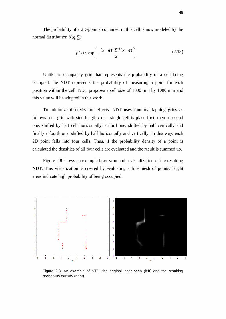
Figure 2.8 shows an example laser scan and a visualization of the resulting
NDT. This visualization is created by evaluating a fine mesh of points; bright
areas indicate high probability of being occupied.
Figure 2.8: An example of NTD: the original laser scan (left) and the resulting
probability density (right).
47
The spatial transformation T between two robot positions is given by:
y
x
t
t
y
x
y
xT
cossin
sincos
'
':
(2.14)
where tx and ty describes the translation and ϕ the rotation between the two
positions. As described in Section 2.3 the goal of the scan matching is to recover
these values using the laser scans taken at two positions. The outline of NTD,
given two scans, is as follows:
1. first, the NDT of the first is built;
2. a estimate for the variables (tx ,ty ,ϕ), is initialized (by zero or by using
odometry data);
3. for each point of the second scan: a reconstructed 2D point into the
coordinate frame of the first scan is mapped, according to the value of
variables;
4. the corresponding normal distribution for each mapped point is
determined;
5. the score for the variables is determined by evaluating the distribution for
each mapped point and summing the result;
6. a new estimate for variables are calculated by trying to optimize the score,
this is done by performing one step of Newton’s Algorithm, and
7. go to step 3 until a convergence criterion is met.
The steps one to four are straightforward. The remaining is described using
the following notation:
p = (tx ,ty ,ϕ)T
: the vector of the variables to estimate.
xi : the reconstructed 2D point of laser scan point i of the second scan in
the coordinate frame of the second scan.
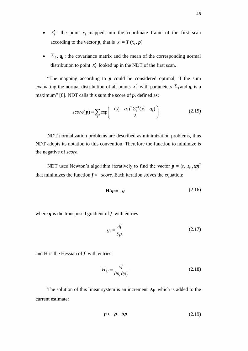
48
ix : the point xi mapped into the coordinate frame of the first scan
according to the vector p, that is ix = T (xi , p)
i , qi : the covariance matrix and the mean of the corresponding normal
distribution to point ix looked up in the NDT of the first scan.
“The mapping according to p could be considered optimal, if the sum
evaluating the normal distribution of all points ix with parameters i and qi is a
maximum” [8]. NDT calls this sum the score of p, defined as:
i
iiii qxqxscore
2
)(Σ)(exp)(
1
i
T
p (2.15)
NDT normalization problems are described as minimization problems, thus
NDT adopts its notation to this convention. Therefore the function to minimize is
the negative of score.
NDT uses Newton’s algorithm iteratively to find the vector p = (tx ,ty ,ϕ)T
that minimizes the function f = –score. Each iteration solves the equation:
gp ΔH (2.16)
where g is the transposed gradient of f with entries
i
ip
fg
(2.17)
and H is the Hessian of f with entries
ji
jipp
fH
(2.18)
The solution of this linear system is an increment pΔ which is added to the
current estimate:
ppp Δ (2.19)

49
2.4. Genetic Algorithms
The Genetic Algorithm (GA) is a search heuristic that imitates the process
of natural evolution; this heuristic is routinely used to generate useful solutions to
optimization and search problems. Problem solving using genetic algorithms isn´t
new, the pioneering work of J. H. Holland in the 1970’s [14] showed significant
contribution for engineering applications.
GA´s are inspired by a biological process in which best individuals are
likely to be the winners in a competing environment. The potential solution of a
problem is an individual which can be represented by a set of variables. These
variables are considered as the genes of a chromosome and they are usually
structured by a sequence of bits. A positive value (known as fitness value),
obtained by a Fitness Function, reflects the degree of “quality” of the
chromosome in order to solve the problem, and this value is narrowly related to its
objective value.
In the process of a genetic evolution, a chromosome with high quality has
the tendency to produce good-quality offsprings, which means better solutions to
the problem. “In a practical application of GA, a population pool of chromosomes
has to be installed, which can be randomly set initially” [15]. In each cycle of
genetic process, a subsequent generation is created from the best chromosomes in
the current population. This group of chromosomes, generally called “parents”,
are selected via a specific selection routine. The roulette wheel selection [16] is
one of the most commonly used techniques to provide selection mechanism; this
selection is based on the fitness value of chromosomes.
The parents are mixed and recombined to produce offsprings for the next
generation. From this process of evolution, it is expected that the best
chromosomes will create more offsprings, and thus having a higher probability of
surviving in the subsequent generation. This emulates the survival-of-the-fittest
mechanism in nature. The evolution cycle is repeated until a desired termination
criterion is reached. The criterion used could be the number of evolution cycles,
the amount of variation of individuals between different generations, or a
50
predefined fitness value. In order to achieve a GA evolution cycle, two
fundamental operators, crossover and mutation, are required.
The procedure described above can be applied in many different ways to
solve a wide range of problems.
However, in the design of a GA to solve a specific problem, there are
always two major decisions: specifying the mapping between the chromosome
structure and candidate solutions (representation problem) and defining a concrete
fitness function.
2.4.1. Chromosome Representation
“Bit-string encoding is the most classical approach used by GA researchers
because of its simplicity and traceability” [15]. A slight modification is the use of
Gray code in the binary coding; “in practice, Gray-coded representation if often
more successful for multi-variable function optimization applications” [17].
Real-valued chromosomes were introduced to deal with real variable
problems. “Many works indicate that the floating point representation would be
faster in computation” [15].
2.4.2. The Fitness Function
“The Fitness Function is at the heart of an evolutionary computing
application” [18]. It determines which solutions within a population are better at
solving the particular problem[18], being an important link between GA and the
system. The Fitness Function takes a chromosome as an input and outputs a
number which represents the measure of the chromosome performance.
An ideal fitness function correlates closely with the algorithm goal, and
besides may be computed quickly. Speed of execution is very important, thus, a
51
typical GA must be iterated many, many times, in order to produce a usable result
for a non-trivial problem.
Definition of the Fitness Function is not straightforward in many cases, and
it is often performed iteratively if the solutions produced by GA are not what it is
desired.
2.4.3. Fundamental Operators
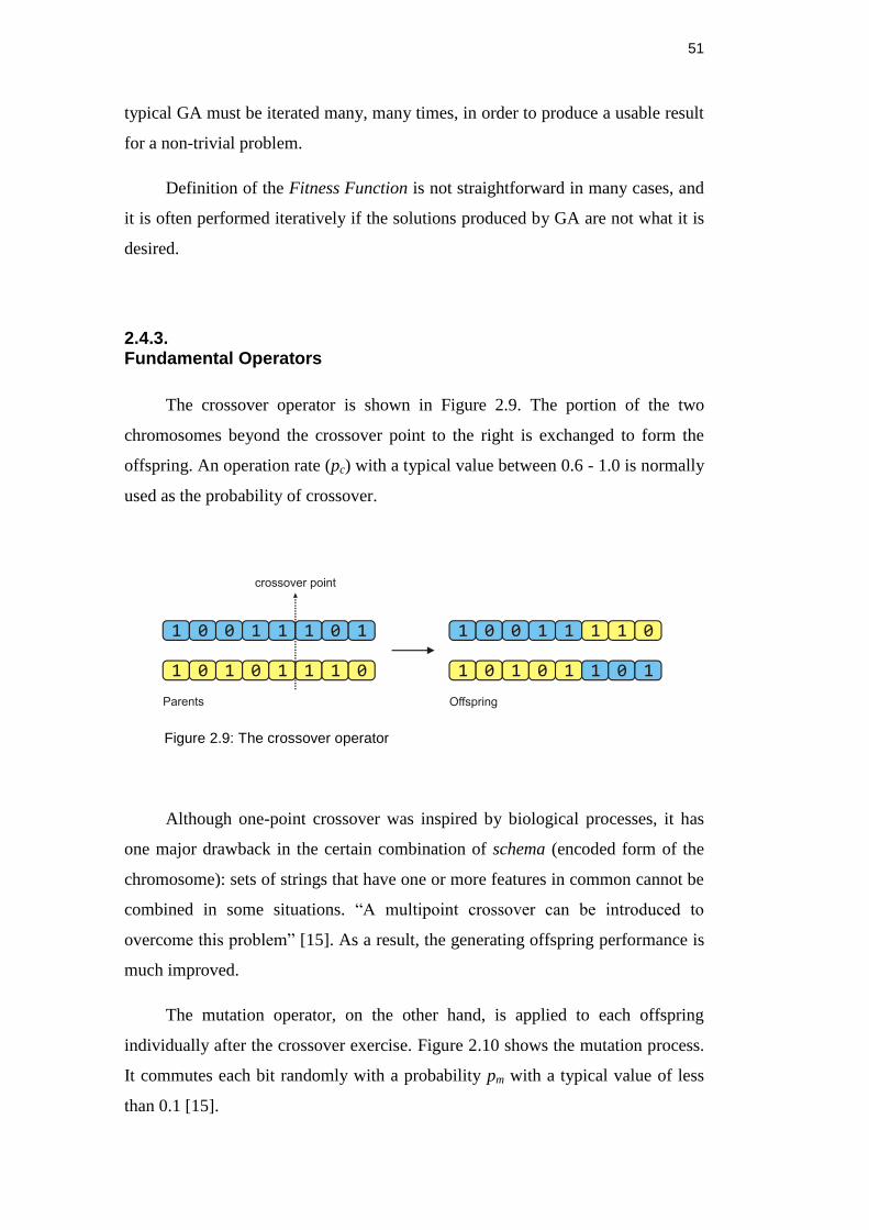
The crossover operator is shown in Figure 2.9. The portion of the two
chromosomes beyond the crossover point to the right is exchanged to form the
offspring. An operation rate (pc) with a typical value between 0.6 - 1.0 is normally
used as the probability of crossover.
Figure 2.9: The crossover operator
Although one-point crossover was inspired by biological processes, it has
one major drawback in the certain combination of schema (encoded form of the
chromosome): sets of strings that have one or more features in common cannot be
combined in some situations. “A multipoint crossover can be introduced to
overcome this problem” [15]. As a result, the generating offspring performance is
much improved.
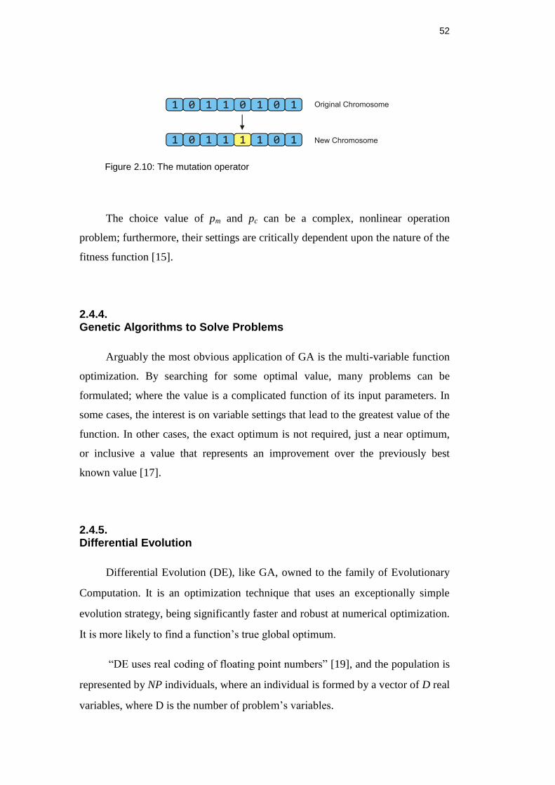
The mutation operator, on the other hand, is applied to each offspring
individually after the crossover exercise. Figure 2.10 shows the mutation process.
It commutes each bit randomly with a probability pm with a typical value of less
than 0.1 [15].
52
Figure 2.10: The mutation operator
The choice value of pm and pc can be a complex, nonlinear operation
problem; furthermore, their settings are critically dependent upon the nature of the
fitness function [15].
2.4.4. Genetic Algorithms to Solve Problems
Arguably the most obvious application of GA is the multi-variable function
optimization. By searching for some optimal value, many problems can be
formulated; where the value is a complicated function of its input parameters. In
some cases, the interest is on variable settings that lead to the greatest value of the
function. In other cases, the exact optimum is not required, just a near optimum,
or inclusive a value that represents an improvement over the previously best
known value [17].
2.4.5. Differential Evolution
Differential Evolution (DE), like GA, owned to the family of Evolutionary
Computation. It is an optimization technique that uses an exceptionally simple
evolution strategy, being significantly faster and robust at numerical optimization.
It is more likely to find a function’s true global optimum.
“DE uses real coding of floating point numbers” [19], and the population is
represented by NP individuals, where an individual is formed by a vector of D real
variables, where D is the number of problem’s variables.
53
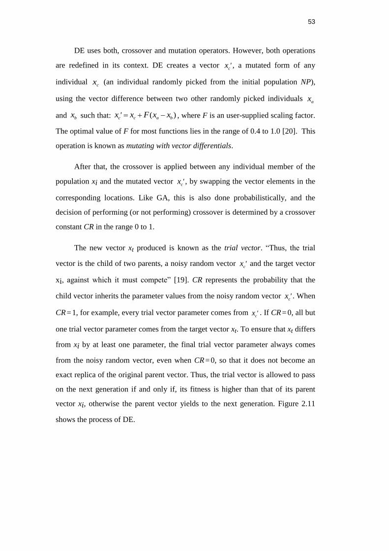
DE uses both, crossover and mutation operators. However, both operations
are redefined in its context. DE creates a vector 'cx , a mutated form of any
individual cx (an individual randomly picked from the initial population NP),
using the vector difference between two other randomly picked individuals ax
and bx such that: )( bacc xxFxx ' , where F is an user-supplied scaling factor.
The optimal value of F for most functions lies in the range of 0.4 to 1.0 [20]. This
operation is known as mutating with vector differentials.
After that, the crossover is applied between any individual member of the
population xi and the mutated vector 'cx , by swapping the vector elements in the
corresponding locations. Like GA, this is also done probabilistically, and the
decision of performing (or not performing) crossover is determined by a crossover
constant CR in the range 0 to 1.
The new vector xt produced is known as the trial vector. “Thus, the trial
vector is the child of two parents, a noisy random vector 'cx and the target vector
xi, against which it must compete” [19]. CR represents the probability that the
child vector inherits the parameter values from the noisy random vector 'cx . When
CR = 1, for example, every trial vector parameter comes from 'cx . If CR = 0, all but
one trial vector parameter comes from the target vector xt. To ensure that xt differs
from xi by at least one parameter, the final trial vector parameter always comes
from the noisy random vector, even when CR = 0, so that it does not become an
exact replica of the original parent vector. Thus, the trial vector is allowed to pass
on the next generation if and only if, its fitness is higher than that of its parent
vector xi, otherwise the parent vector yields to the next generation. Figure 2.11
shows the process of DE.
54
Figure 2.11: Differential Evolution Process [21]
Among all, just three factors control evolution under DE: the population
size NP, the weight F applied to the random differential, and the crossover
constant CR.
2.4.6. Different Strategies of DE
Depending on the type of problem, different strategies can be adopted in the
DE algorithm. “The strategies can vary based on the vector to be perturbed,
number of difference vectors considered for perturbation, and finally the type of
crossover used” [19]. The following are the 10 different working strategies
proposed by Price and Storn [21].
1. DE/best/1/exp
55
2. DE/rand/1/exp
3. DE/rand-to-best/1/exp
4. DE/best/2/exp
5. DE/rand/2/exp
6. DE/best/1/bin
7. DE/rand/1/bin
8. DE/rand-to-best/1/bin
9. DE/best/2/bin
10. DE/rand/2/bin
The convention used above is DE/x/y/z. DE means Differential Evolution, x
denotes a string representing the vector to be perturbed, y is the number of
difference vectors used for perturbation of x, and z denotes the type of crossover
being used (exp: exponential, bin: binomial).
For perturbation with a single vector difference, out of the three distinct
randomly chosen vectors, the weighted vector differential of any two vectors is
added to the third one. In the same way for perturbation with two vector
differences, five distinct vectors, other than the target vector, are chosen randomly
from the current population. Out of these, the weighted vector difference of each
pair of any four vectors is added to the fifth one for perturbation.
In exponential crossover, the crossover is performed on the D variables in
one loop until it is within the CR bound. In binomial crossover, the crossover is
performed on each of the D variables whenever a randomly picked number
between 0 and 1 is within the CR value. So, for high values of CR, the exponential
and binomial crossovers yield similar results. In the binomial case, the last
variable always comes from a random noisy vector to ensure that is different from
the target vector, and hence the above procedure is applied up to D – 1 variables.
“The strategy to be adopted for each problem is to be determined separately
by trial and error” [19]. The best strategy for a given problem may not work well
when applied to a different problem.
In the next chapter, the presented analytical background is applied to the
SLAM problem.
56
3. SLAM Solutions
3.1. Gaussian Filter SLAM Solutions
“Historically, Gaussian Filters constitute the earliest tractable
implementations of the Bayes Filter for continuous spaces”. It could say that they
are also by far the most popular family of techniques to date – despite a number of
limitations [1].
Gaussian assumes the idea that beliefs are represented by multivariate
normal distributions:
)}()(exp{)2det()( 1
212
1
xxxp T (3.1)
The distribution over the variable x is characterized by two sets of
parameters: the mean λ and the covariance Σ. The mean has the same
dimensionality of the state x. The covariance is a symmetric quadratic matrix,
positive semi-definite, and its dimension is the dimensionality of the state x
squared. Hence, the dimension of the covariance matrix depends quadratically on
the dimension of the state vector x.
3.1.1. Kalman Filter SLAM
“Probably the best studied technique for implementing Bayes filter is the
Kalman Filter” [1]. “The Kalman Filter (KF) was developed by R.E. Kalman,
whose prominent paper on the subject was published in 1960” [4].
The KF is an algorithm which processes data and estimates variable values.
In SLAM context, the variable values to be estimated consist of the robot position
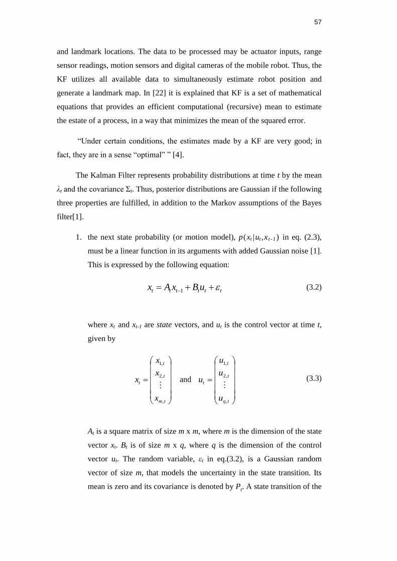
57
and landmark locations. The data to be processed may be actuator inputs, range
sensor readings, motion sensors and digital cameras of the mobile robot. Thus, the
KF utilizes all available data to simultaneously estimate robot position and
generate a landmark map. In [22] it is explained that KF is a set of mathematical
equations that provides an efficient computational (recursive) mean to estimate
the estate of a process, in a way that minimizes the mean of the squared error.
“Under certain conditions, the estimates made by a KF are very good; in
fact, they are in a sense “optimal” ” [4].
The Kalman Filter represents probability distributions at time t by the mean
λt and the covariance Σt. Thus, posterior distributions are Gaussian if the following
three properties are fulfilled, in addition to the Markov assumptions of the Bayes
filter[1].
1. the next state probability (or motion model), p(xt |ut ,x t -1) in eq. (2.3),
must be a linear function in its arguments with added Gaussian noise [1].
This is expressed by the following equation:
tttttt uBxAx 1 (3.2)
where xt and xt-1 are state vectors, and ut is the control vector at time t,
given by
tm
t
t
t
x
x
x
x
,
,2
,1
and
tq
t
t
t
u
u
u
u
,
,2
,1
(3.3)
At is a square matrix of size m x m, where m is the dimension of the state
vector xt. Bt is of size m x q, where q is the dimension of the control
vector ut. The random variable, εt in eq.(3.2), is a Gaussian random
vector of size m, that models the uncertainty in the state transition. Its
mean is zero and its covariance is denoted by Pt. A state transition of the
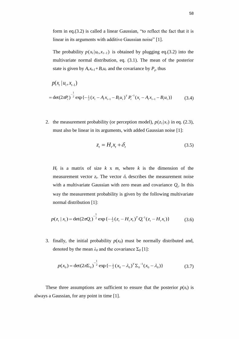
58
form in eq.(3.2) is called a linear Gaussian, “to reflect the fact that it is
linear in its arguments with additive Gaussian noise” [1].
The probability p(xt |ut ,x t -1) is obtained by plugging eq.(3.2) into the
multivariate normal distribution, eq. (3.1). The mean of the posterior
state is given by Atxt-1+Btut and the covariance by Pt, thus
),|( 1ttt xuxp
)}()(exp{)2det( 1
1
1212
1
tttttt
T
tttttt uBxAxPuBxAxP
(3.4)
2. the measurement probability (or perception model), p(z t|x t) in eq. (2.3),
must also be linear in its arguments, with added Gaussian noise [1]:
tttt xHz (3.5)
Ht is a matrix of size k x m, where k is the dimension of the
measurement vector zt. The vector δt describes the measurement noise
with a multivariate Gaussian with zero mean and covariance Qt. In this
way the measurement probability is given by the following multivariate
normal distribution [1]:
)}()(exp{)2det()|( 1
212
1
tttt
T
tttttt xHzQxHzQxzp
(3.6)
3. finally, the initial probability p(x0) must be normally distributed and,
denoted by the mean λ0 and the covariance Σ0 [1]:
)}()(exp{)2det()( 00
1
000212
1
00
xxxp T
(3.7)
These three assumptions are sufficient to ensure that the posterior p(xt) is
always a Gaussian, for any point in time [1].
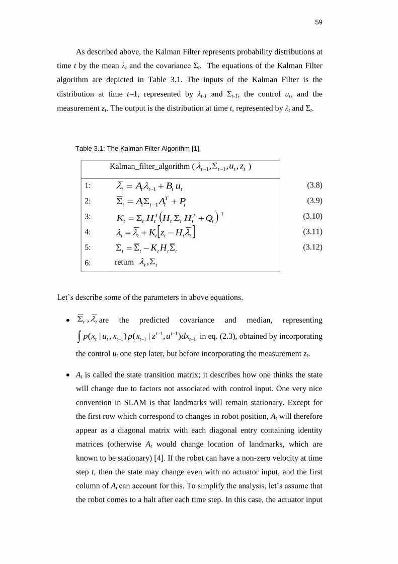
59
As described above, the Kalman Filter represents probability distributions at
time t by the mean λt and the covariance Σt. The equations of the Kalman Filter
algorithm are depicted in Table 3.1. The inputs of the Kalman Filter is the
distribution at time t1, represented by λt-1 and Σt-1, the control ut, and the
measurement zt. The output is the distribution at time t, represented by λt and Σt.
Table 3.1: The Kalman Filter Algorithm [1].
Kalman_filter_algorithm ( tttt zu ,,, 11 )
1: ttttt uBA 1 (3.8)
2: t
T
tttt PAA 1 (3.9)
3: 1 t
T
ttt
T
ttt QHHHK (3.10)
4: tttttt HzK (3.11)
5: ttttt HK (3.12)
6: return tt ,
Let’s describe some of the parameters in above equations.
tt , are the predicted covariance and median, representing
1
11
11 ),|(),|( t
tt
tttt dxuzxpxuxp in eq. (2.3), obtained by incorporating
the control ut one step later, but before incorporating the measurement zt.
At is called the state transition matrix; it describes how one thinks the state
will change due to factors not associated with control input. One very nice
convention in SLAM is that landmarks will remain stationary. Except for
the first row which correspond to changes in robot position, At will therefore
appear as a diagonal matrix with each diagonal entry containing identity
matrices (otherwise At would change location of landmarks, which are
known to be stationary) [4]. If the robot can have a non-zero velocity at time
step t, then the state may change even with no actuator input, and the first
column of At can account for this. To simplify the analysis, let’s assume that
the robot comes to a halt after each time step. In this case, the actuator input
60
fully specifies the most likely new location of the robot. This means that At
is just the identity matrix, which could be disregarded.
Bt is a matrix that translates control input into a predicted change in state. Its
values will depend on the representation of the control input. It will vary
depending on the physical construction of the robot. Because the landmarks
will remain stationary the only interesting entries of Bt will be in the first
row. Thus, the idea of eq. (3.8) is that the best guess for the new state will
be described exactly by the old robot position and how one believes the
actuators will change this position.
Pt is the covariance of the process noise. It accounts for how moving will
change the confidence on each individual pair of landmarks as well as robot-
landmarks pairs. The entries of Pt will depend on the distance landmarks are
away from the robot and other known particularities of the environment
and/or state [4].
Qt is the covariance matrix for the range sensor noise, it is used to keep
track of one’s confidence in the range sensor readings.
Ht transforms one’s previous state estimate into a representation used by the
sensors. In other words, if the sensors had perceived the world state exactly
as predicted by t , they would have returned this information in the
formttH . Note that the purpose of Ht is very similar to that of Bt.
Finally, Kt is called the Kalman gain. It specifies the degree to which the
measurement is incorporated into the new state estimate. The magnitudes of
the values in Kt depend on the predicted covariancet , relative to the
combined values of the predicted covariance and sensor uncertainty Qt.
The Kalman filter is a technique for filtering and prediction in linear
systems. However, in most real world SLAM situations there will be some non-
linear aspect one might wish to account for. “For example, a robot that moves
with constant translational and rotational velocity typically moves on a circular
trajectory, which cannot be described by linear next estate transitions” [1]. Thus
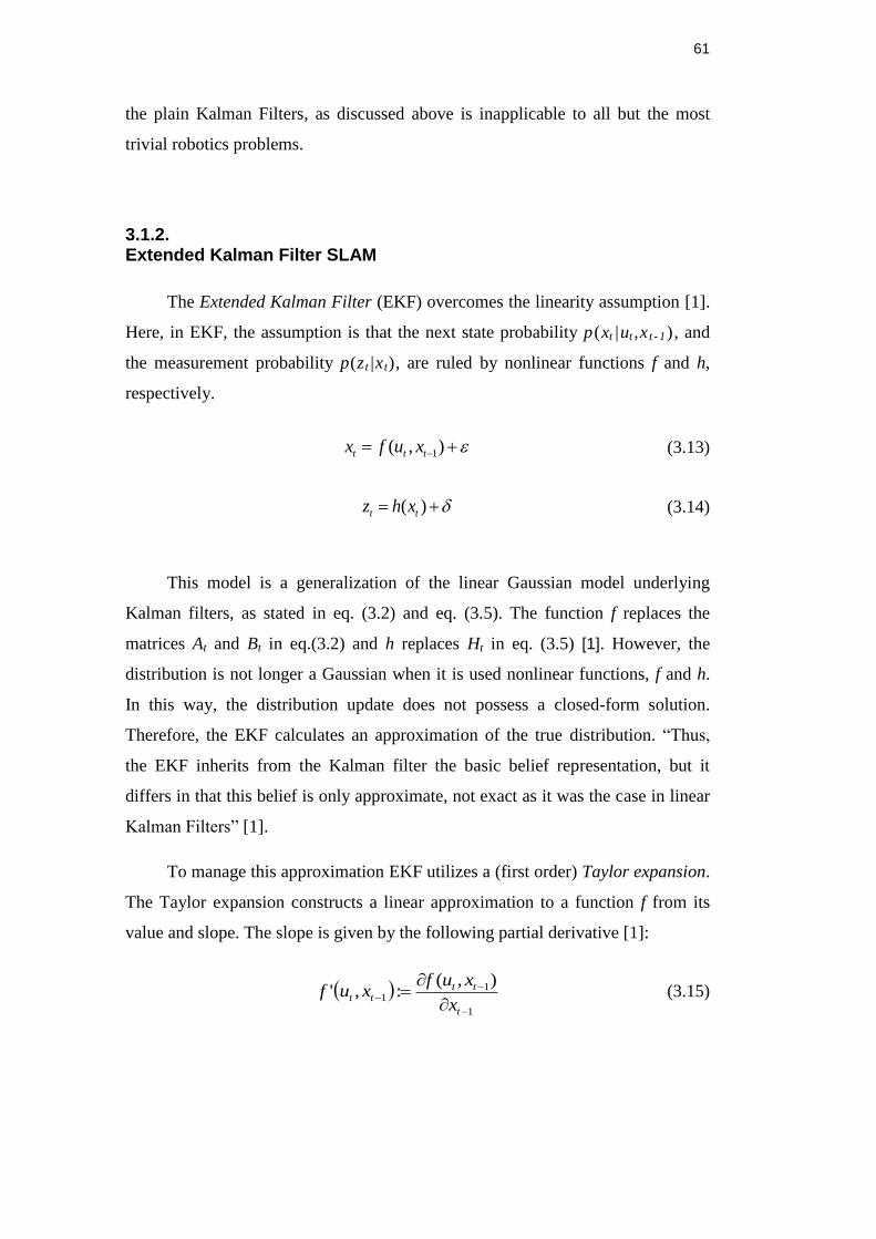
61
the plain Kalman Filters, as discussed above is inapplicable to all but the most
trivial robotics problems.
3.1.2. Extended Kalman Filter SLAM
The Extended Kalman Filter (EKF) overcomes the linearity assumption [1].
Here, in EKF, the assumption is that the next state probability p(xt |ut ,x t - 1), and
the measurement probability p(z t|x t), are ruled by nonlinear functions f and h,
respectively.
),( 1ttt xufx (3.13)
)( tt xhz
(3.14)
This model is a generalization of the linear Gaussian model underlying
Kalman filters, as stated in eq. (3.2) and eq. (3.5). The function f replaces the
matrices At and Bt in eq.(3.2) and h replaces Ht in eq. (3.5) [1]. However, the
distribution is not longer a Gaussian when it is used nonlinear functions, f and h.
In this way, the distribution update does not possess a closed-form solution.
Therefore, the EKF calculates an approximation of the true distribution. “Thus,
the EKF inherits from the Kalman filter the basic belief representation, but it
differs in that this belief is only approximate, not exact as it was the case in linear
Kalman Filters” [1].
To manage this approximation EKF utilizes a (first order) Taylor expansion.
The Taylor expansion constructs a linear approximation to a function f from its
value and slope. The slope is given by the following partial derivative [1]:
1
11
),(:,'
t
tttt
x
xufxuf (3.15)
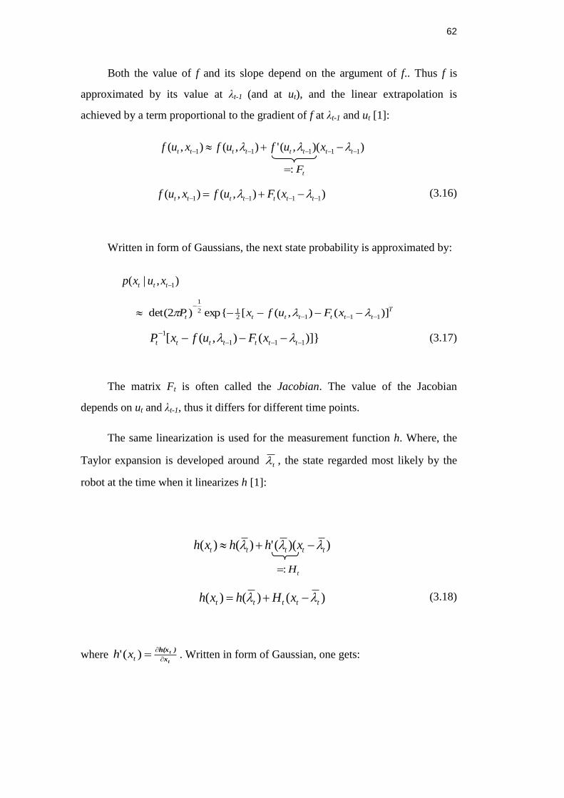
62
Both the value of f and its slope depend on the argument of f.. Thus f is
approximated by its value at λt-1 (and at ut), and the linear extrapolation is
achieved by a term proportional to the gradient of f at λt-1 and ut [1]:
))(,('),(),( 11111 tttttttt xufufxuf
tF:
)(),(),( 1111 ttttttt xFufxuf (3.16)
Written in form of Gaussians, the next state probability is approximated by:
),|( 1ttt xuxp
T
ttttttt xFufxP )](),([exp{)2det( 111212
1
)]}(),([ 111
1
ttttttt xFufxP
(3.17)
The matrix Ft is often called the Jacobian. The value of the Jacobian
depends on ut and λt-1, thus it differs for different time points.
The same linearization is used for the measurement function h. Where, the
Taylor expansion is developed around t , the state regarded most likely by the
robot at the time when it linearizes h [1]:
))((')()( ttttt xhhxh
tH:
)()()( ttttt xHhxh (3.18)
where t
t
x
)h(x
)(' txh . Written in form of Gaussian, one gets:
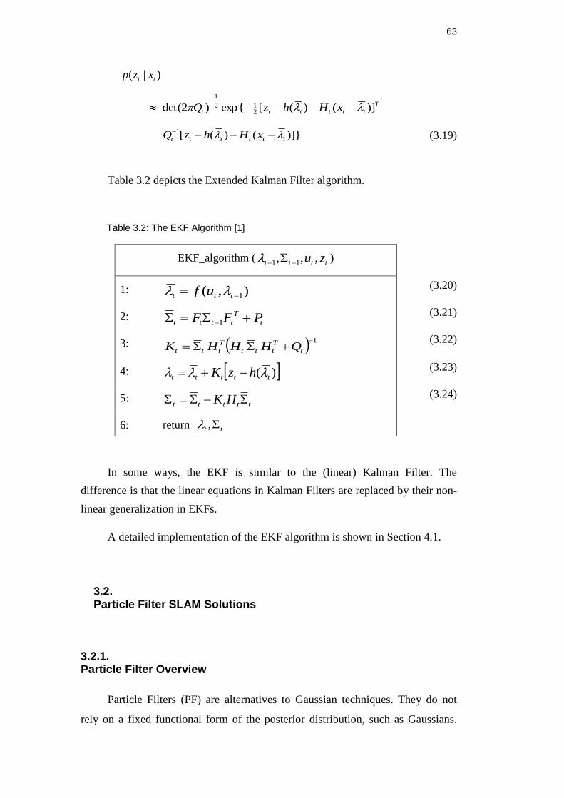
63
)|( tt xzp
T
tttttt xHhzQ )]()([exp{)2det(212
1
)]}()([1
tttttt xHhzQ
(3.19)
Table 3.2 depicts the Extended Kalman Filter algorithm.
Table 3.2: The EKF Algorithm [1]
EKF_algorithm (tttt zu ,,, 11 )
1: ),( 1 ttt uf (3.20)
2: t
T
tttt PFF 1 (3.21)
3: 1 t
T
ttt
T
ttt QHHHK (3.22)
4: )( ttttt hzK (3.23)
5: ttttt HK
(3.24)
6: return tt ,
In some ways, the EKF is similar to the (linear) Kalman Filter. The
difference is that the linear equations in Kalman Filters are replaced by their non-
linear generalization in EKFs.
A detailed implementation of the EKF algorithm is shown in Section 4.1.
3.2. Particle Filter SLAM Solutions
3.2.1. Particle Filter Overview
Particle Filters (PF) are alternatives to Gaussian techniques. They do not
rely on a fixed functional form of the posterior distribution, such as Gaussians.
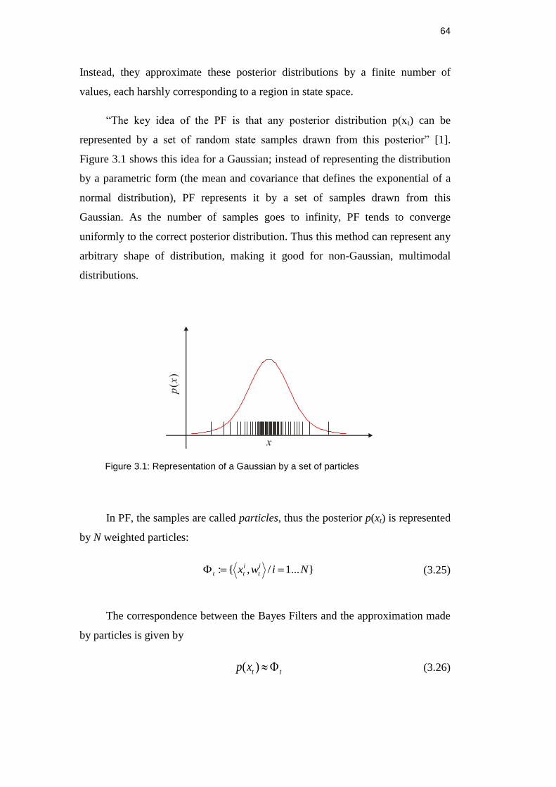
64
Instead, they approximate these posterior distributions by a finite number of
values, each harshly corresponding to a region in state space.
“The key idea of the PF is that any posterior distribution p(xt) can be
represented by a set of random state samples drawn from this posterior” [1].
Figure 3.1 shows this idea for a Gaussian; instead of representing the distribution
by a parametric form (the mean and covariance that defines the exponential of a
normal distribution), PF represents it by a set of samples drawn from this
Gaussian. As the number of samples goes to infinity, PF tends to converge
uniformly to the correct posterior distribution. Thus this method can represent any
arbitrary shape of distribution, making it good for non-Gaussian, multimodal
distributions.
Figure 3.1: Representation of a Gaussian by a set of particles
In PF, the samples are called particles, thus the posterior p(xt) is represented
by N weighted particles:
}...1/,{: Niwx i
t
i
tt (3.25)
The correspondence between the Bayes Filters and the approximation made
by particles is given by
ttxp )( (3.26)
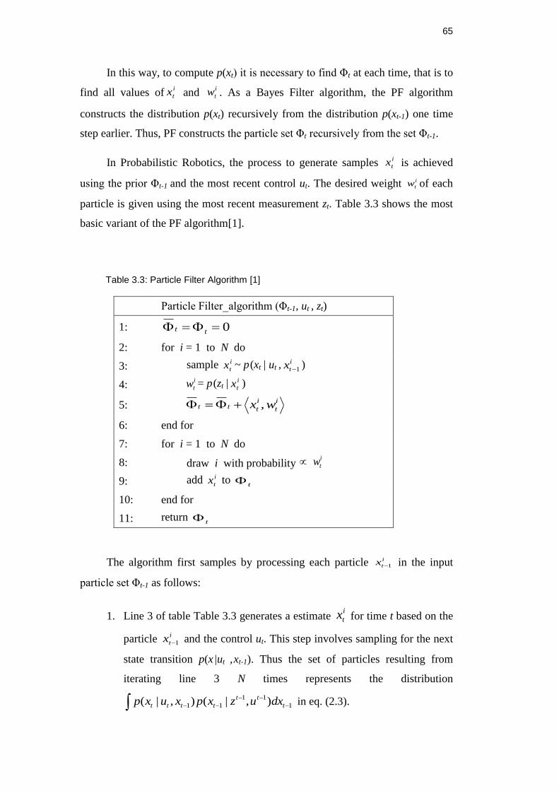
65
In this way, to compute p(xt) it is necessary to find Φt at each time, that is to
find all values ofi
tx and
i
tw . As a Bayes Filter algorithm, the PF algorithm
constructs the distribution p(xt) recursively from the distribution p(xt-1) one time
step earlier. Thus, PF constructs the particle set Φt recursively from the set Φt-1.
In Probabilistic Robotics, the process to generate samples i
tx is achieved
using the prior Φt-1 and the most recent control ut. The desired weight i
tw of each
particle is given using the most recent measurement zt. Table 3.3 shows the most
basic variant of the PF algorithm[1].
Table 3.3: Particle Filter Algorithm [1]
Particle Filter_algorithm (Φt-1, ut , zt)
1: 0 tt
2: for i = 1 to N do
3: sample i
tx ~ p(xt | ut ,i
tx 1)
4: i
tw = p(zt |i
tx )
5: i
t
i
ttt wx ,
6: end for
7: for i = 1 to N do
8: draw i with probability i
tw
9: add i
tx to t
10: end for
11: return t
The algorithm first samples by processing each particle i
tx 1 in the input
particle set Φt-1 as follows:
1. Line 3 of table Table 3.3 generates a estimate i
tx for time t based on the
particle i
tx 1 and the control ut. This step involves sampling for the next
state transition p(x|ut ,xt-1). Thus the set of particles resulting from
iterating line 3 N times represents the distribution
1
11
11 ),|(),|( t
tt
tttt dxuzxpxuxp in eq. (2.3).
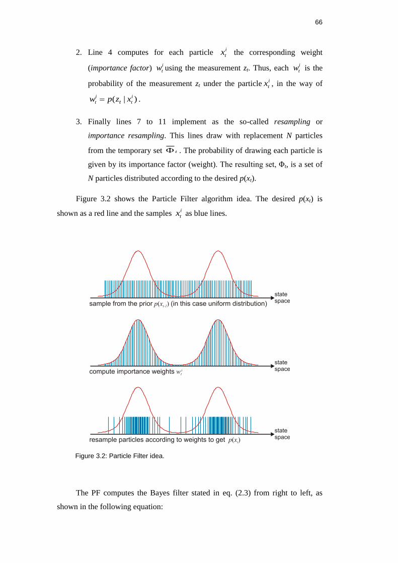
66
2. Line 4 computes for each particle i
tx the corresponding weight
(importance factor) i
tw using the measurement zt. Thus, each i
tw is the
probability of the measurement zt under the particlei
tx , in the way of
)|( i
t
i
t xzpw t .
3. Finally lines 7 to 11 implement as the so-called resampling or
importance resampling. This lines draw with replacement N particles
from the temporary set t . The probability of drawing each particle is
given by its importance factor (weight). The resulting set, Φt, is a set of
N particles distributed according to the desired p(xt).
Figure 3.2 shows the Particle Filter algorithm idea. The desired p(xt) is
shown as a red line and the samples i
tx as blue lines.
Figure 3.2: Particle Filter idea.
The PF computes the Bayes filter stated in eq. (2.3) from right to left, as
shown in the following equation:
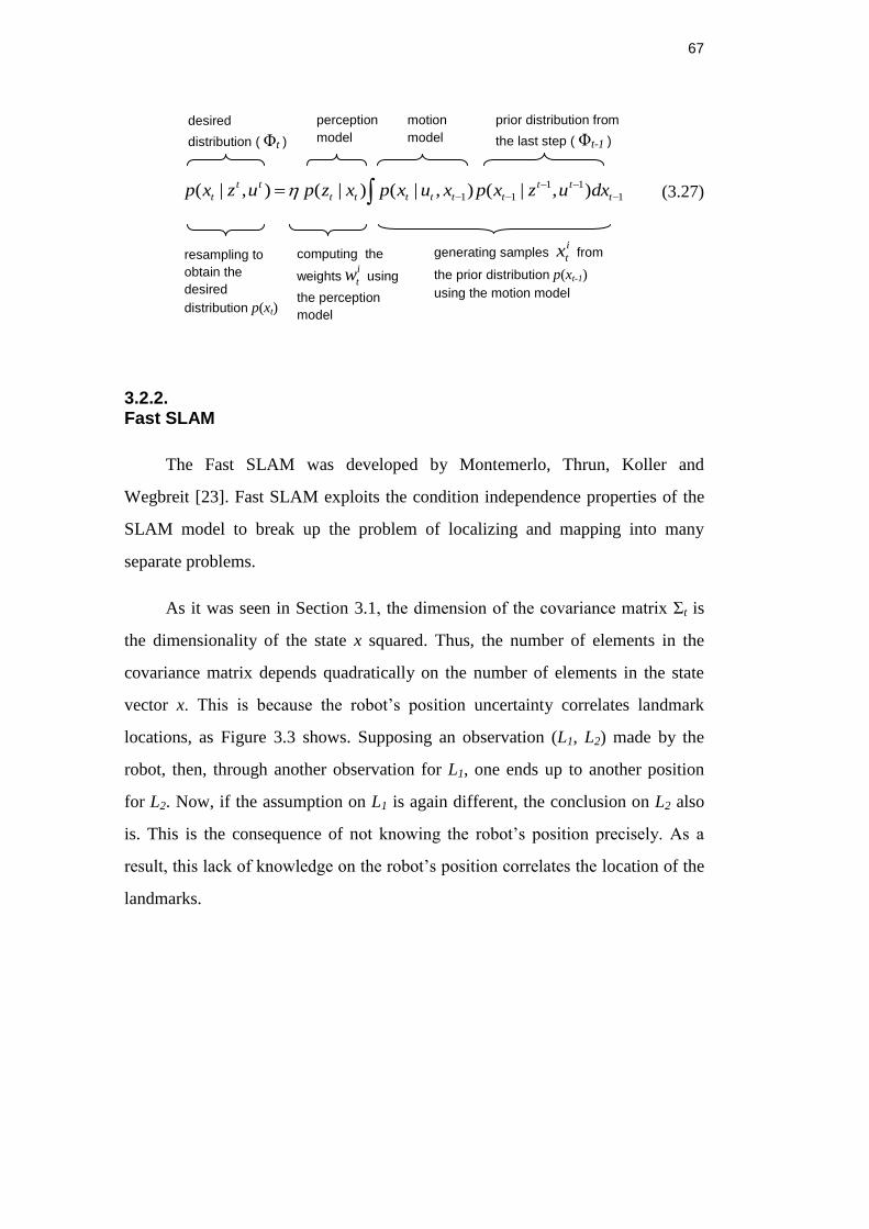
67
1
11
11 ),|(),|()|(),|( t
tt
tttttt
tt
t dxuzxpxuxpxzpuzxp
(3.27)
3.2.2. Fast SLAM
The Fast SLAM was developed by Montemerlo, Thrun, Koller and
Wegbreit [23]. Fast SLAM exploits the condition independence properties of the
SLAM model to break up the problem of localizing and mapping into many
separate problems.
As it was seen in Section 3.1, the dimension of the covariance matrix Σt is
the dimensionality of the state x squared. Thus, the number of elements in the
covariance matrix depends quadratically on the number of elements in the state
vector x. This is because the robot’s position uncertainty correlates landmark
locations, as Figure 3.3 shows. Supposing an observation (L1, L2) made by the
robot, then, through another observation for L1, one ends up to another position
for L2. Now, if the assumption on L1 is again different, the conclusion on L2 also
is. This is the consequence of not knowing the robot’s position precisely. As a
result, this lack of knowledge on the robot’s position correlates the location of the
landmarks.
generating samples i
tx from
the prior distribution p(xt-1)
using the motion model
computing the
weightsi
tw using
the perception
model
resampling to
obtain the
desired
distribution p(xt)
prior distribution from
the last step ( Φt-1 )
motion
model
perception
model
desired
distribution ( Φt )
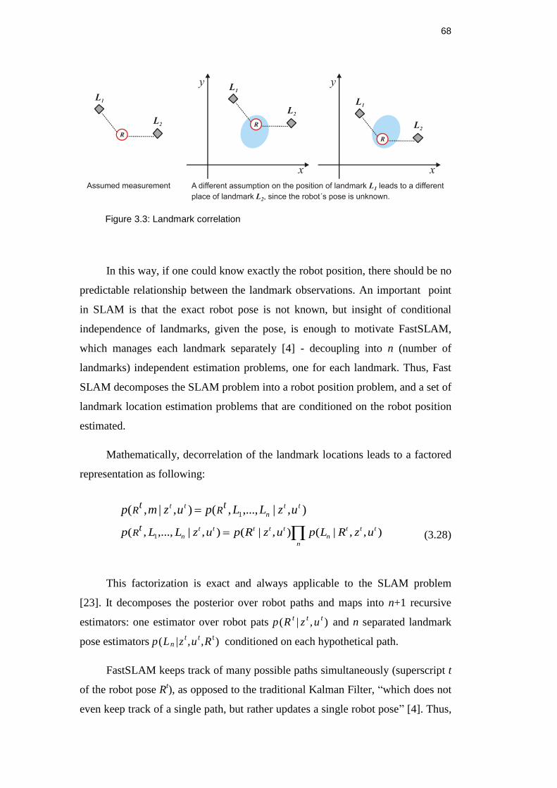
68
Figure 3.3: Landmark correlation
In this way, if one could know exactly the robot position, there should be no
predictable relationship between the landmark observations. An important point
in SLAM is that the exact robot pose is not known, but insight of conditional
independence of landmarks, given the pose, is enough to motivate FastSLAM,
which manages each landmark separately [4] - decoupling into n (number of
landmarks) independent estimation problems, one for each landmark. Thus, Fast
SLAM decomposes the SLAM problem into a robot position problem, and a set of
landmark location estimation problems that are conditioned on the robot position
estimated.
Mathematically, decorrelation of the landmark locations leads to a factored
representation as following:
),|,...,,(),|,( 1
tt
n
tt uzLLpuzmp tR
tR
n
ttt
n
ttttt
n uzRLpuzRpuzLLp tR ),,|(),|(),|,...,,( 1 (3.28)
This factorization is exact and always applicable to the SLAM problem
[23]. It decomposes the posterior over robot paths and maps into n+1 recursive
estimators: one estimator over robot pats p(Rt| z
t, u
t) and n separated landmark
pose estimators p(Ln |zt,u
t,R
t) conditioned on each hypothetical path.
FastSLAM keeps track of many possible paths simultaneously (superscript t
of the robot pose Rt), as opposed to the traditional Kalman Filter, “which does not
even keep track of a single path, but rather updates a single robot pose” [4]. Thus,
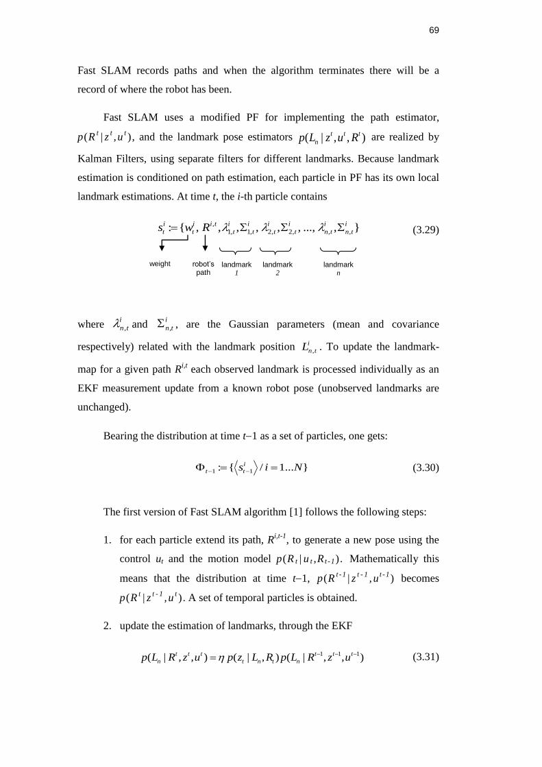
69
Fast SLAM records paths and when the algorithm terminates there will be a
record of where the robot has been.
Fast SLAM uses a modified PF for implementing the path estimator,
p(Rt| z
t,u
t), and the landmark pose estimators ),,|( ttt
n RuzLp are realized by
Kalman Filters, using separate filters for different landmarks. Because landmark
estimation is conditioned on path estimation, each particle in PF has its own local
landmark estimations. At time t, the i-th particle contains
},...,,,,,,,{: ,,,2,2,1,1
, i
tn
i
tn
i
t
i
t
i
t
i
t
tii
t
i
t Rws (3.29)
where i
tn, and i
tn, , are the Gaussian parameters (mean and covariance
respectively) related with the landmark position i
tnL , . To update the landmark-
map for a given path Ri,t
each observed landmark is processed individually as an
EKF measurement update from a known robot pose (unobserved landmarks are
unchanged).
Bearing the distribution at time t1 as a set of particles, one gets:
}...1/{: 11 Nisi
tt (3.30)
The first version of Fast SLAM algorithm [1] follows the following steps:
1. for each particle extend its path, Ri,t-1
, to generate a new pose using the
control ut and the motion model p(R t | u t ,R t -1). Mathematically this
means that the distribution at time t1, p(Rt -1
| zt - 1
, ut -1
) becomes
p(Rt| z
t - 1, u
t). A set of temporal particles is obtained.
2. update the estimation of landmarks, through the EKF
),,|(),|(),,|( 111 ttt
ntnt
ttt
n uzRLpRLzpuzRLp (3.31)
weight robot’s path
landmark 1
landmark 2
landmark n
70
and, using the new poses generated in the step 1 and the measurement zt,
compute the new set of ,
i
n t and ,
i
n t . This set of means and covariances
are added to the temporal particles set.
3. assign the weight for each particle. This is computed using the result of
step 1, p(Rt| z
t - 1, u
t), where the measurement zt was not included, and
using the distribution p(Rt| z
t,u
t), where zt is included
),|(
),|(1,
,
ttit
ttiti
tuzRp
uzRpw
(3.32)
after some considerations and probabilistic transformations, the above
equation is given by:
)}ˆ()ˆ(exp{)2det( 1
212
1
i
tt
i
t
Ti
tt
i
t
i
t zzUzzUw
(3.33)
QHHU i
t
i
nt
Ti
t
i
t ,1 (3.34)
where zt is the sensor observation. Note that i
tz is the predicted
observation computed using the landmark position estimated in step 2
and the robot poses generated in step 1. i
tH is the Jacobian of the
perception model. This set of importance factors (weights) are added to
the temporal particles set.
4. finally, resample. Each particle, in the temporal particle set, is drawn
(with replacement) with a probability proportional to its importance
factor.
A detailed implementation of the Fast Slam 1.0 algorithm is shown in
Section 4.2.

71
3.2.3. DP-SLAM
The Fast SLAM is a good solution to the SLAM problem when there are
thousands of landmarks that can be tracked accurately. However tracking
landmarks is actually very difficult, particularly in environments with
monochromatic areas or repeating patterns.
If the robot is using a LRF, the map generated by the laser has no
landmarks; is rather an occupancy grid, as described in Section 2.2.2. “The robot
cannot use the range finder to relocate individual points in the grid. However with
enough data, the robot might not need to worry about reacquiring landmarks in the
first place” [4]. For example, if there was a contoured object in the environment,
the robot might align entire occupancy maps by matching up the contour of that
object. Distributed Particle SLAM (DP-SLAM) [6] attacks SLAM from this
occupancy grid approach, while simultaneously utilizing the conditional
independence insight discussed in Fast SLAM.
“One of the steps in the Fast SLAM algorithm was to generate a new pose
prediction and a corresponding map prediction” [4]. Thus, the new map prediction
was based on the previous pose and the control input ut. It cannot predict how
landmarks will move with respect to the robot anymore because landmarks are not
dealt with. However it is possible to make a prediction as to how the occupancy
grid will change. Figure 3.4 shows an example of occupancy grid prediction based
on a movement of one cell to the right.
Figure 3.4: Occupancy grid prediction based on a movement of one cell to the right.
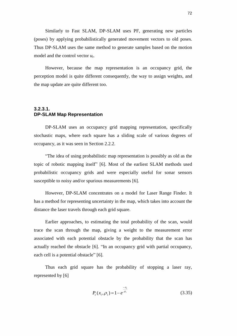
72
Similarly to Fast SLAM, DP-SLAM uses PF, generating new particles
(poses) by applying probabilistically generated movement vectors to old poses.
Thus DP-SLAM uses the same method to generate samples based on the motion
model and the control vector ut.
However, because the map representation is an occupancy grid, the
perception model is quite different consequently, the way to assign weights, and
the map update are quite different too.
3.2.3.1. DP-SLAM Map Representation
DP-SLAM uses an occupancy grid mapping representation, specifically
stochastic maps, where each square has a sliding scale of various degrees of
occupancy, as it was seen in Section 2.2.2.
“The idea of using probabilistic map representation is possibly as old as the
topic of robotic mapping itself” [6]. Most of the earliest SLAM methods used
probabilistic occupancy grids and were especially useful for sonar sensors
susceptible to noisy and/or spurious measurements [6].
However, DP-SLAM concentrates on a model for Laser Range Finder. It
has a method for representing uncertainty in the map, which takes into account the
distance the laser travels through each grid square.
Earlier approaches, to estimating the total probability of the scan, would
trace the scan through the map, giving a weight to the measurement error
associated with each potential obstacle by the probability that the scan has
actually reached the obstacle [6]. “In an occupancy grid with partial occupancy,
each cell is a potential obstacle” [6].
Thus each grid square has the probability of stopping a laser ray,
represented by [6]
i
ix
iic exP
1),( (3.35)
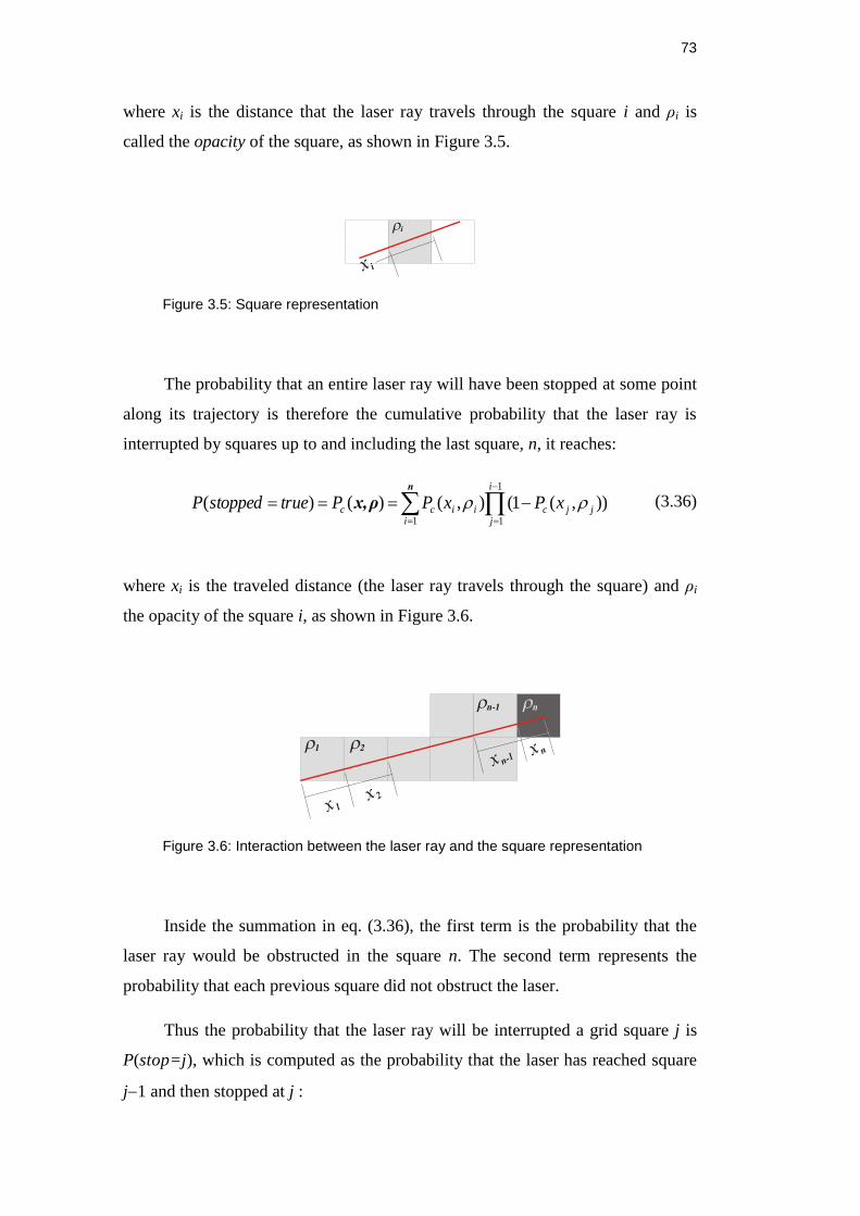
73
where xi is the distance that the laser ray travels through the square i and ρi is
called the opacity of the square, as shown in Figure 3.5.
Figure 3.5: Square representation
The probability that an entire laser ray will have been stopped at some point
along its trajectory is therefore the cumulative probability that the laser ray is
interrupted by squares up to and including the last square, n, it reaches:
n
ρx,1
1
1
)),(1(),()()(i
i
jjjciicc xPxPPtruestoppedP (3.36)
where xi is the traveled distance (the laser ray travels through the square) and ρi
the opacity of the square i, as shown in Figure 3.6.
Figure 3.6: Interaction between the laser ray and the square representation
Inside the summation in eq. (3.36), the first term is the probability that the
laser ray would be obstructed in the square n. The second term represents the
probability that each previous square did not obstruct the laser.
Thus the probability that the laser ray will be interrupted a grid square j is
P(stop=j), which is computed as the probability that the laser has reached square
j1 and then stopped at j :
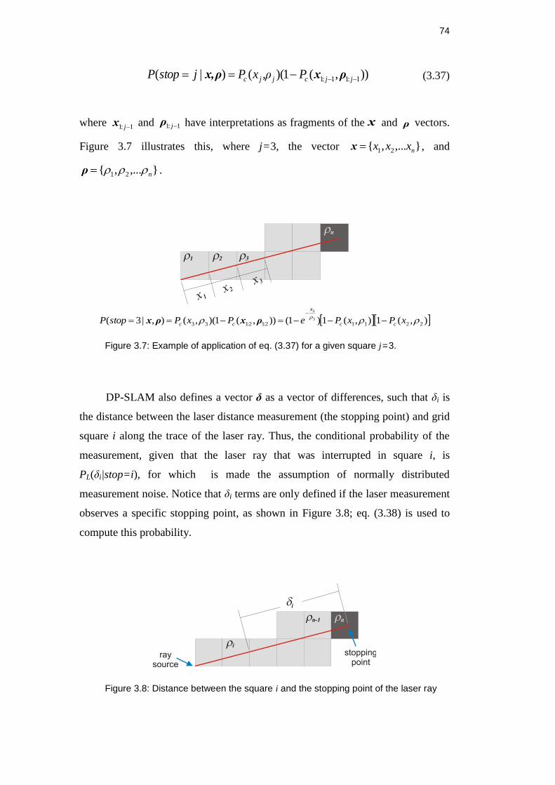
74
)),(1)(()|( 1:11:1 jjcjjc P,ρxPjstopP ρxρx, (3.37)
where 1:1 jx and 1:1 jρ have interpretations as fragments of the x and ρ vectors.
Figure 3.7 illustrates this, where j=3, the vector },...,{ 21 nxxxx , and
},...,{ 21 nρ .
),(1),(1)1()),(1)(,(),|3( 22112:12:1333
3
xPxPePxPstopP cc
x
cc
ρρ xx
Figure 3.7: Example of application of eq. (3.37) for a given square j=3.
DP-SLAM also defines a vector δ as a vector of differences, such that δi is
the distance between the laser distance measurement (the stopping point) and grid
square i along the trace of the laser ray. Thus, the conditional probability of the
measurement, given that the laser ray that was interrupted in square i, is
PL(δi|stop=i), for which is made the assumption of normally distributed
measurement noise. Notice that δi terms are only defined if the laser measurement
observes a specific stopping point, as shown in Figure 3.8; eq. (3.38) is used to
compute this probability.
Figure 3.8: Distance between the square i and the stopping point of the laser ray
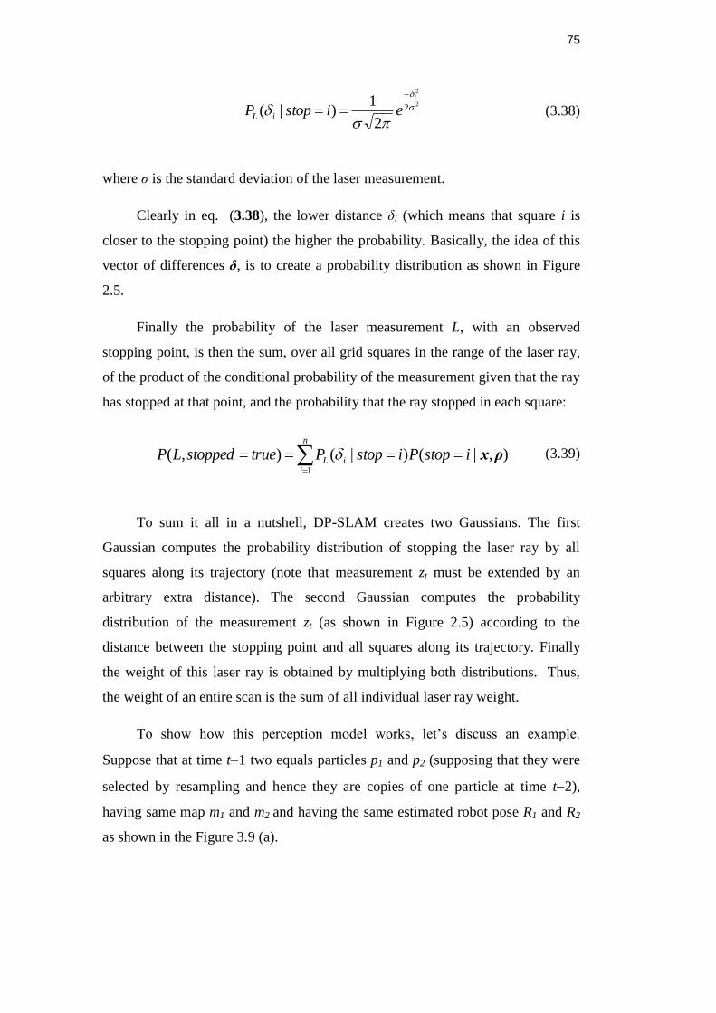
75
2
2
2
2
1)|(
i
eistopP iL
(3.38)
where σ is the standard deviation of the laser measurement.
Clearly in eq. (3.38), the lower distance δi (which means that square i is
closer to the stopping point) the higher the probability. Basically, the idea of this
vector of differences δ, is to create a probability distribution as shown in Figure
2.5.
Finally the probability of the laser measurement L, with an observed
stopping point, is then the sum, over all grid squares in the range of the laser ray,
of the product of the conditional probability of the measurement given that the ray
has stopped at that point, and the probability that the ray stopped in each square:
n
iiL istopPistopPtruestoppedLP
1
),|()|(),( ρx (3.39)
To sum it all in a nutshell, DP-SLAM creates two Gaussians. The first
Gaussian computes the probability distribution of stopping the laser ray by all
squares along its trajectory (note that measurement zt must be extended by an
arbitrary extra distance). The second Gaussian computes the probability
distribution of the measurement zt (as shown in Figure 2.5) according to the
distance between the stopping point and all squares along its trajectory. Finally
the weight of this laser ray is obtained by multiplying both distributions. Thus,
the weight of an entire scan is the sum of all individual laser ray weight.
To show how this perception model works, let’s discuss an example.
Suppose that at time t1 two equals particles p1 and p2 (supposing that they were
selected by resampling and hence they are copies of one particle at time t2),
having same map m1 and m2 and having the same estimated robot pose R1 and R2
as shown in the Figure 3.9 (a).
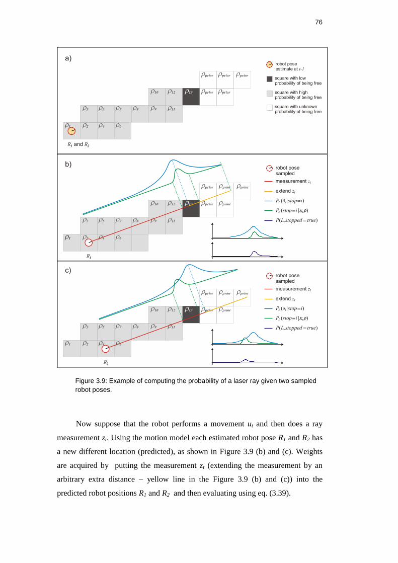
76
Figure 3.9: Example of computing the probability of a laser ray given two sampled
robot poses.
Now suppose that the robot performs a movement ut and then does a ray
measurement zt. Using the motion model each estimated robot pose R1 and R2 has
a new different location (predicted), as shown in Figure 3.9 (b) and (c). Weights
are acquired by putting the measurement zt (extending the measurement by an
arbitrary extra distance – yellow line in the Figure 3.9 (b) and (c)) into the
predicted robot positions R1 and R2 and then evaluating using eq. (3.39).
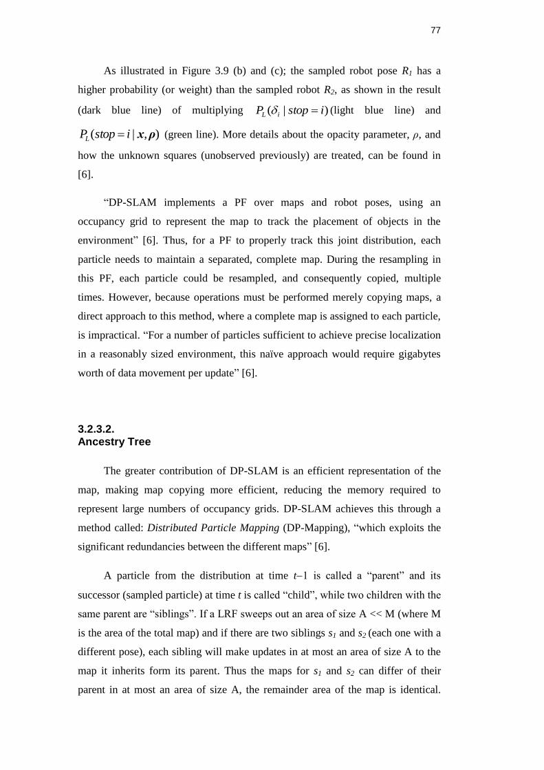
77
As illustrated in Figure 3.9 (b) and (c); the sampled robot pose R1 has a
higher probability (or weight) than the sampled robot R2, as shown in the result
(dark blue line) of multiplying )|( istopP iL (light blue line) and
),|( ρxistopPL (green line). More details about the opacity parameter, ρ, and
how the unknown squares (unobserved previously) are treated, can be found in
[6].
“DP-SLAM implements a PF over maps and robot poses, using an
occupancy grid to represent the map to track the placement of objects in the
environment” [6]. Thus, for a PF to properly track this joint distribution, each
particle needs to maintain a separated, complete map. During the resampling in
this PF, each particle could be resampled, and consequently copied, multiple
times. However, because operations must be performed merely copying maps, a
direct approach to this method, where a complete map is assigned to each particle,
is impractical. “For a number of particles sufficient to achieve precise localization
in a reasonably sized environment, this naïve approach would require gigabytes
worth of data movement per update” [6].
3.2.3.2. Ancestry Tree
The greater contribution of DP-SLAM is an efficient representation of the
map, making map copying more efficient, reducing the memory required to
represent large numbers of occupancy grids. DP-SLAM achieves this through a
method called: Distributed Particle Mapping (DP-Mapping), “which exploits the
significant redundancies between the different maps” [6].
A particle from the distribution at time t1 is called a “parent” and its
successor (sampled particle) at time t is called “child”, while two children with the
same parent are “siblings”. If a LRF sweeps out an area of size A << M (where M
is the area of the total map) and if there are two siblings s1 and s2 (each one with a
different pose), each sibling will make updates in at most an area of size A to the
map it inherits form its parent. Thus the maps for s1 and s2 can differ of their
parent in at most an area of size A, the remainder area of the map is identical.
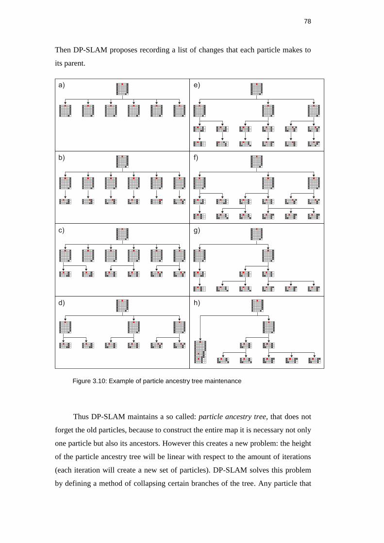
78
Then DP-SLAM proposes recording a list of changes that each particle makes to
its parent.
Figure 3.10: Example of particle ancestry tree maintenance
Thus DP-SLAM maintains a so called: particle ancestry tree, that does not
forget the old particles, because to construct the entire map it is necessary not only
one particle but also its ancestors. However this creates a new problem: the height
of the particle ancestry tree will be linear with respect to the amount of iterations
(each iteration will create a new set of particles). DP-SLAM solves this problem
by defining a method of collapsing certain branches of the tree. Any particle that
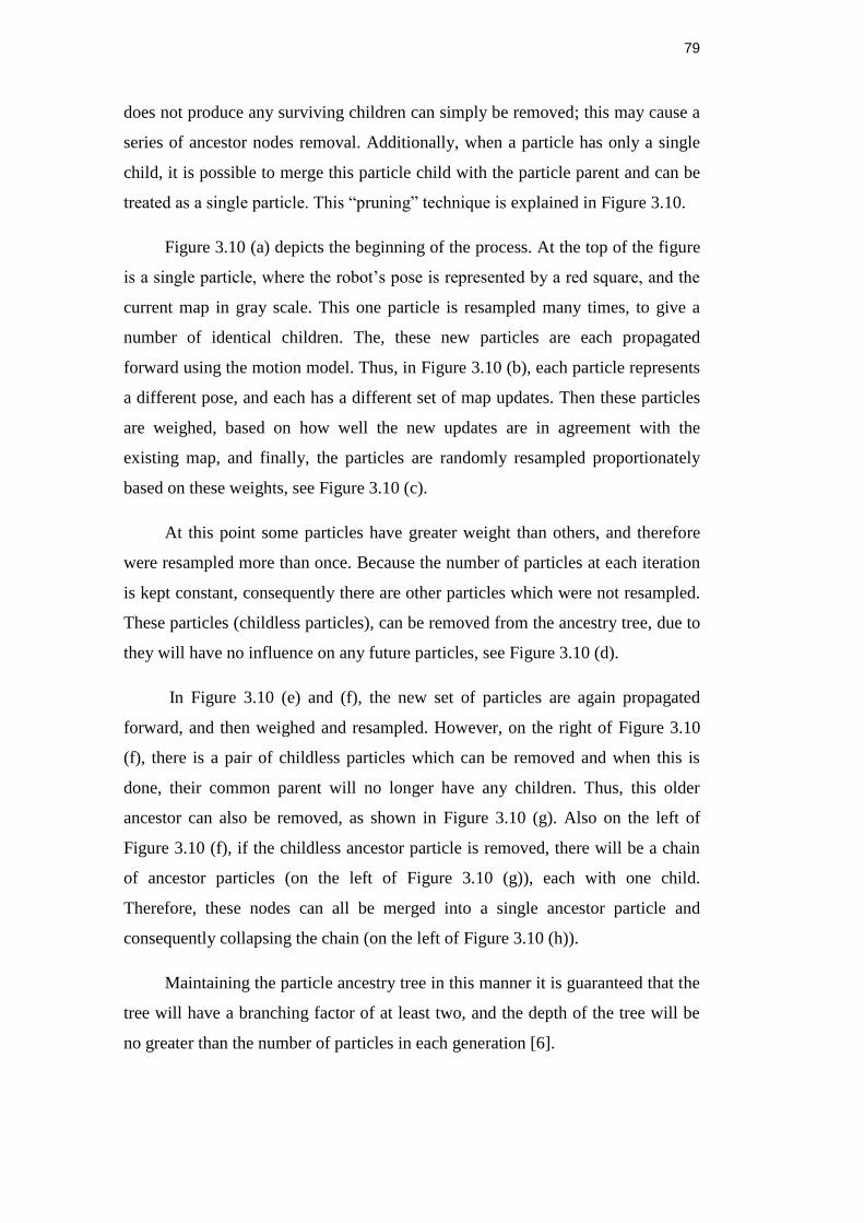
79
does not produce any surviving children can simply be removed; this may cause a
series of ancestor nodes removal. Additionally, when a particle has only a single
child, it is possible to merge this particle child with the particle parent and can be
treated as a single particle. This “pruning” technique is explained in Figure 3.10.
Figure 3.10 (a) depicts the beginning of the process. At the top of the figure
is a single particle, where the robot’s pose is represented by a red square, and the
current map in gray scale. This one particle is resampled many times, to give a
number of identical children. The, these new particles are each propagated
forward using the motion model. Thus, in Figure 3.10 (b), each particle represents
a different pose, and each has a different set of map updates. Then these particles
are weighed, based on how well the new updates are in agreement with the
existing map, and finally, the particles are randomly resampled proportionately
based on these weights, see Figure 3.10 (c).
At this point some particles have greater weight than others, and therefore
were resampled more than once. Because the number of particles at each iteration
is kept constant, consequently there are other particles which were not resampled.
These particles (childless particles), can be removed from the ancestry tree, due to
they will have no influence on any future particles, see Figure 3.10 (d).
In Figure 3.10 (e) and (f), the new set of particles are again propagated
forward, and then weighed and resampled. However, on the right of Figure 3.10
(f), there is a pair of childless particles which can be removed and when this is
done, their common parent will no longer have any children. Thus, this older
ancestor can also be removed, as shown in Figure 3.10 (g). Also on the left of
Figure 3.10 (f), if the childless ancestor particle is removed, there will be a chain
of ancestor particles (on the left of Figure 3.10 (g)), each with one child.
Therefore, these nodes can all be merged into a single ancestor particle and
consequently collapsing the chain (on the left of Figure 3.10 (h)).
Maintaining the particle ancestry tree in this manner it is guaranteed that the
tree will have a branching factor of at least two, and the depth of the tree will be
no greater than the number of particles in each generation [6].
80
3.2.3.3. Hierarchical SLAM
The DP-SLAM provides an accurate and efficient method for building
maps. However, there are some trajectories, which cover a sufficient amount of
distance before completing a cycle, for which the accuracy of the map can
degrade [6]. Small errors are accumulated over several iterations, and although the
resulting map may look locally consistent, there is a large total error, which is
more evident when the robot closes a large loop. This behavior over large
distances is known as “drift”. It is a significant problem faced by essentially all
current SLAM algorithms [6].
As a consequence of violated assumptions or as a consequence of particle
filtering it is hard to avoid drift. Errors come from three sources: insufficient
number of particles, coarse precision, and resampling itself (particle depletion).
The consequence of these errors is a gradual but inevitable accumulation resulting
from faults to sample, differentiate, or remember a state vector that is sufficiently
close to the true state.
Figure 3.11: Simulated environment (60 x 40 m).
81
Figure 3.11 shows a loop-closed simulated environment. This map consists
of 183 LRF scans. It was build using DP-SLAM (without hierarchical SLAM)
with 2800 particles. This loop is large enough that particle diversity is insufficient
to correct the small errors that occur.
The reason that a non-hierarchical method cannot manage this data is the
extreme longevity of the uncertainty. In a large loop, small ambiguities in the
beginning of the map are not resolved for many thousand iterations [6]. Non
hierarchical DP-SLAM requires a huge number of particles to maintain this early
particle diversity.
3.2.3.4. Hierarchical Algorithm
DP-SLAM uses two levels Hierarchical-SLAM where the lowest level
models the physical process (SLAM itself), while the higher level models errors
in the lower level.
“Since the total drift over trajectory is assumed to be a summation of many
small, largely independent sources of error, it can be well approximated by
Gaussian distribution” [6]. Thus DP-SLAM states that the effects of drift on low
level maps can be precisely approximated by perturbations on the robot’s
trajectory endpoints used to construct a low level map.
DP-SLAM uses a standard SLAM algorithm for the low level mapping
process. The low level algorithm input is a small portion of the robot’s trajectory,
along with the associated observations (range scans). This low level SLAM
process runs normally, and its output (a trajectory) is treated as distribution over
motions (motion model) in the higher level SLAM process, to which additional
noise from drift is added. So the output from each of small mapping is the input
for a new SLAM process, working at a higher level of time steps.
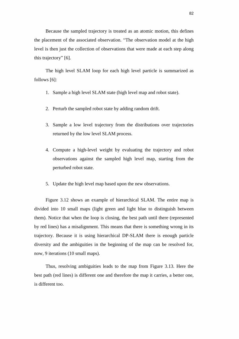
82
Because the sampled trajectory is treated as an atomic motion, this defines
the placement of the associated observation. “The observation model at the high
level is then just the collection of observations that were made at each step along
this trajectory” [6].
The high level SLAM loop for each high level particle is summarized as
follows [6]:
1. Sample a high level SLAM state (high level map and robot state).
2. Perturb the sampled robot state by adding random drift.
3. Sample a low level trajectory from the distributions over trajectories
returned by the low level SLAM process.
4. Compute a high-level weight by evaluating the trajectory and robot
observations against the sampled high level map, starting from the
perturbed robot state.
5. Update the high level map based upon the new observations.
Figure 3.12 shows an example of hierarchical SLAM. The entire map is
divided into 10 small maps (light green and light blue to distinguish between
them). Notice that when the loop is closing, the best path until there (represented
by red lines) has a misalignment. This means that there is something wrong in its
trajectory. Because it is using hierarchical DP-SLAM there is enough particle
diversity and the ambiguities in the beginning of the map can be resolved for,
now, 9 iterations (10 small maps).
Thus, resolving ambiguities leads to the map from Figure 3.13. Here the
best path (red lines) is different one and therefore the map it carries, a better one,
is different too.
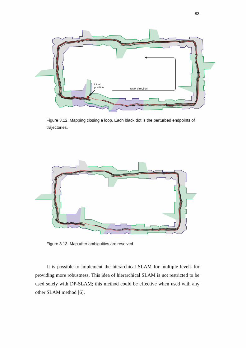
83
Figure 3.12: Mapping closing a loop. Each black dot is the perturbed endpoints of
trajectories.
Figure 3.13: Map after ambiguities are resolved.
It is possible to implement the hierarchical SLAM for multiple levels for
providing more robustness. This idea of hierarchical SLAM is not restricted to be
used solely with DP-SLAM; this method could be effective when used with any
other SLAM method [6].
84
3.3. 3D SLAM Review
Existing SLAM methods produce a two-dimensional cross section of the
world, and robot motion is restricted to motion within this plane. However the
assumption of a 2D world is unrealistic: wheeled robots traveling across uneven
terrain and underwater autonomous vehicles, can all move with six degrees of
freedom, three translational and three angular. For robots to operate in this
environment, it is not only need to track these three new degrees of motion, but
also to maintain a three dimensional representation of the environment.
3D mapping has some advantages compared with 2D [1]:
3D maps facilitate navigation. Many robot environments possess significant
variation in occupancy in the vertical dimension. Modeling this can greatly
reduce the danger of colliding with an obstacle.
Many robot tasks require three-dimensional information, such as tasks
involving the localization and retrieval of objects or people.
3D maps carry much information for a potential user of the maps. If one
builds a map only for the sake or robot navigation, then the SLAM
enforcements would be very few. However, if the map is acquired for later
use by a person, 3D information can be absolutely critical.
Some methods exist for three-dimensional motion. They tend to represent
the world in terms of a few sparse, pint-sized landmarks. These maps, while
useful for localization, and possible for navigation, give very little information
about the presence of objects in the world. In [24] a SLAM framework based on
3D landmarks for indoor environment with stereo vision is shown. Reference [25]
shows a real-time 3D SLAM is constructed using wide-angle vision.
Carnegie Mellon University´s Mine Mapping project is a notable example
of volumetric three dimensional maps, using a series of LRF set at different angles
[26]. Using a combined method of both local and global scan matching
techniques, a two-dimensional occupancy grid is created. Thus, with the
corresponding trajectory from the robot, the remaining three-dimensional data are
85
filled in to create the volumetric maps. Reference [27] presents an EKF-based 3D
SLAM, which uses planar features probabilistically extracted from dense three-
dimensional point clouds generated by a rotated 2D LRF. A similar work [28]
presents SLAM from visual landmarks and 3D planes, modeling the environment
as a set of planar surfaces and lines. These planar surfaces and lines are extracted
by fusing data from a camera and a 3D LRF.
Also DP-SLAM [6] proposes a 3D grid map representation. This
representation brings two types of challenges, technical and dimensional. The
technical problems are mainly issues of sensing. In particular, odometry is unable
to detect any motion in the three new degrees of freedom. The dimensional
challenges arise from a new dimension added to the problem. The resources
needed to deal with SLAM grow exponentially, so that merely extending previous
methods is infeasible on any computer architecture.
However, this thesis is focused in indoor structured environments.
Assuming a flat terrain, the localization given by the 2D DP-SLAM, can be used
to project the corresponding 3D points. Thus a 3D map is constructed, composed
by a set of points (a point cloud). This proposed method has similarities with the
one presented in [26] where 3D maps are obtained by using the 2D pose
information via the geometric projections.
Chapter 5 will show some results by applying DP-SLAM in simulated data.
After creating a 2D map, the DP-SLAM algorithm gives the best estimated path.
Using this, the corresponding 3D points are projected. The implemented simulator
is discussed in detail in the next chapter.
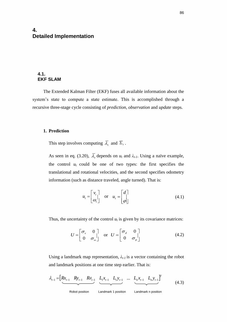
86
4. Detailed Implementation
4.1. EKF SLAM
The Extended Kalman Filter (EKF) fuses all available information about the
system’s state to compute a state estimate. This is accomplished through a
recursive three-stage cycle consisting of prediction, observation and update steps.
1. Prediction
This step involves computing t and t .
As seen in eq. (3.20), t depends on ut and λt-1. Using a naïve example,
the control ut could be one of two types: the first specifies the
translational and rotational velocities, and the second specifies odometry
information (such as distance traveled, angle turned). That is:
ort
t
t
vu
dut
(4.1)
Thus, the uncertainty of the control ut is given by its covariance matrices:
0
or0
vU
0
0dU
(4.2)
Using a landmark map representation, λt-1 is a vector containing the robot
and landmark positions at one time step earlier. That is:
Ttntntttttt yLxLyLxLRRyRx 1111111111 ...
Robot position Landmark 1 position Landmark n position
(4.3)
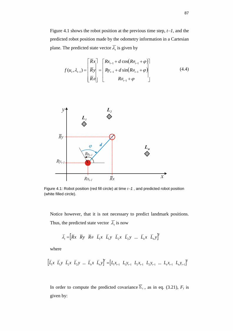
87
Figure 4.1 shows the robot position at the previous time step, t1, and the
predicted robot position made by the odometry information in a Cartesian
plane. The predicted state vectort is given by
1
11
11
1 sin
cos
),(
t
tt
tt
tt
R
RdRy
RdRx
R
yR
xR
uf
(4.4)
Figure 4.1: Robot position (red fill circle) at time t1 , and predicted robot position
(white filled circle).
Notice however, that it is not necessary to predict landmark positions.
Thus, the predicted state vector t is now
Tnnt yLxLyLxLyLxLRyRxR ...2211
where
Ttntntttt
T
nn yLxLyLxLyLxLyLxLyLxLyLxL 11121211112211 ......
In order to compute the predicted covariance t , as in eq. (3.21), Ft is
given by:
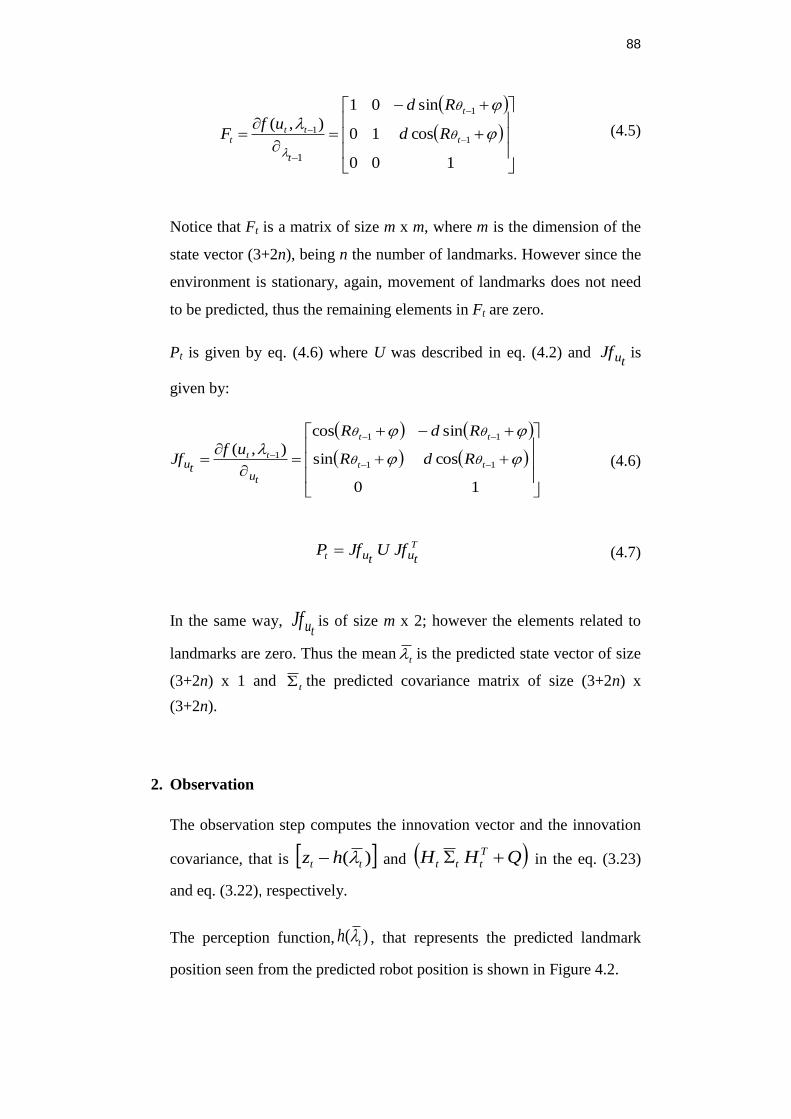
88
100
cos10
sin01
),(1
1
1
1
t
t
ttt Rd
Rd
ufF
t
(4.5)
Notice that Ft is a matrix of size m x m, where m is the dimension of the
state vector (3+2n), being n the number of landmarks. However since the
environment is stationary, again, movement of landmarks does not need
to be predicted, thus the remaining elements in Ft are zero.
Pt is given by eq. (4.6) where U was described in eq. (4.2) and tuJf is
given by:
10
cossin
sincos
),(11
11
1
tt
tt
tt RdR
RdR
ufJf
tutu
(4.6)
T
t tutu JfUJfP
(4.7)
In the same way, tuJf is of size m x 2; however the elements related to
landmarks are zero. Thus the meant is the predicted state vector of size
(3+2n) x 1 and t the predicted covariance matrix of size (3+2n) x
(3+2n).
2. Observation
The observation step computes the innovation vector and the innovation
covariance, that is )( tt hz and QHH T
ttt in the eq. (3.23)
and eq. (3.22), respectively.
The perception function, )( th , that represents the predicted landmark
position seen from the predicted robot position is shown in Figure 4.2.
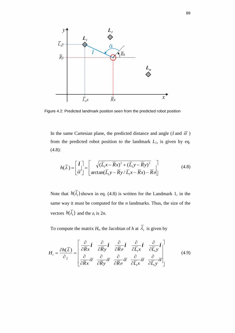
89
Figure 4.2: Predicted landmark position seen from the predicted robot position
In the same Cartesian plane, the predicted distance and angle ( l and )
from the predicted robot position to the landmark L1, is given by eq.
(4.8):
RxRxLyRyL
yRyLxRxLh
)/arctan(
)()()(
11
2
1
2
1l
(4.8)
Note that )( th shown in eq. (4.8) is written for the Landmark 1, in the
same way it must be computed for the n landmarks. Thus, the size of the
vectors )( th and the zt is 2n.
To compute the matrix Ht, the Jacobian of h at t is given by
yLxLRyRxR
yLxLRyRxRhH t
11
11)(lllll
(4.9)
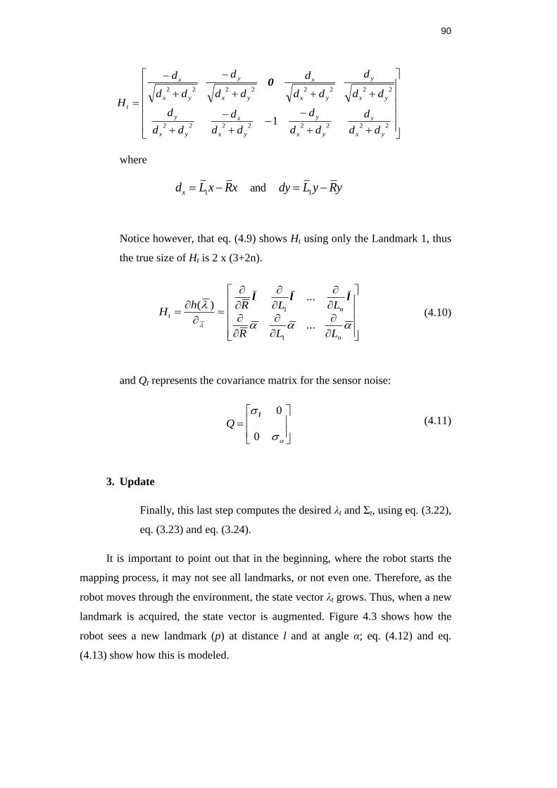
90
22222222
22222222
1yx
x
yx
y
yx
x
yx
y
yx
y
yx
x
yx
y
yx
x
t
dd
d
dd
d
dd
d
dd
d
dd
d
dd
d
dd
d
dd
d
H
0
where
1 1andxd L x Rx dy L y Ry
Notice however, that eq. (4.9) shows Ht using only the Landmark 1, thus
the true size of Ht is 2 x (3+2n).
n
nt
LLR
LLRhH
...
...)(
1
1
lll
(4.10)
and Qt represents the covariance matrix for the sensor noise:
0
0l
Q
(4.11)
3. Update
Finally, this last step computes the desired λt and Σt, using eq. (3.22),
eq. (3.23) and eq. (3.24).
It is important to point out that in the beginning, where the robot starts the
mapping process, it may not see all landmarks, or not even one. Therefore, as the
robot moves through the environment, the state vector λt grows. Thus, when a new
landmark is acquired, the state vector is augmented. Figure 4.3 shows how the
robot sees a new landmark (p) at distance l and at angle α; eq. (4.12) and eq.
(4.13) show how this is modeled.
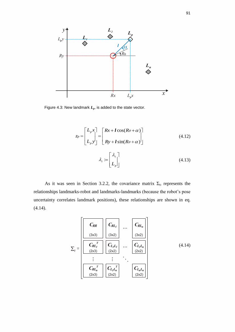
91
Figure 4.3: New landmark Lp, is added to the state vector.
)sin(
)cos(
RRy
RRx
yL
xL
z
p
p
p
l
l
(4.12)
p
t
tL
:
(4.13)
As it was seen in Section 3.2.2, the covariance matrix Σt, represents the
relationships landmarks-robot and landmarks-landmarks (because the robot’s pose
uncertainty correlates landmark positions), these relationships are shown in eq.
(4.14).
(4.14)
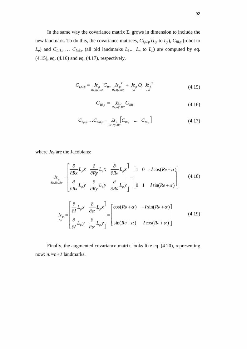
92
In the same way the covariance matrix Σt grows in dimension to include the
new landmark. To do this, the covariance matrices, CLpLp (Lp to Lp), CRLp (robot to
Lp) and CL1Lp … CLnLp (all old landmarks L1… Ln to Lp) are computed by eq.
(4.15), eq. (4.16) and eq. (4.17), respectively.
,,,,,, l
T
ptl
pRRyRx
T
pRRRRyRx
pLpLp JzQJzJzCJzC
(4.15)
RR
RRyRxRLp CJzC p
,,
(4.16)
nRLRLRRyRx
pLnLpLpL CCJzCC ...11
,,
(4.17)
where Jzp are the Jacobians:
)sin(10
)cos(01
,,
R
R
yLR
yLRy
yLRx
xLR
xLRy
xLRx
Jz
ppp
ppp
RRyRx
p
l
l-
(4.18)
)cos()sin(
)sin()cos(
,
RR
RR
yLyL
xLxL
Jz
pp
pp
l
p
l
l
l
l
(4.19)
Finally, the augmented covariance matrix looks like eq. (4.20), representing
now: n:=n+1 landmarks.
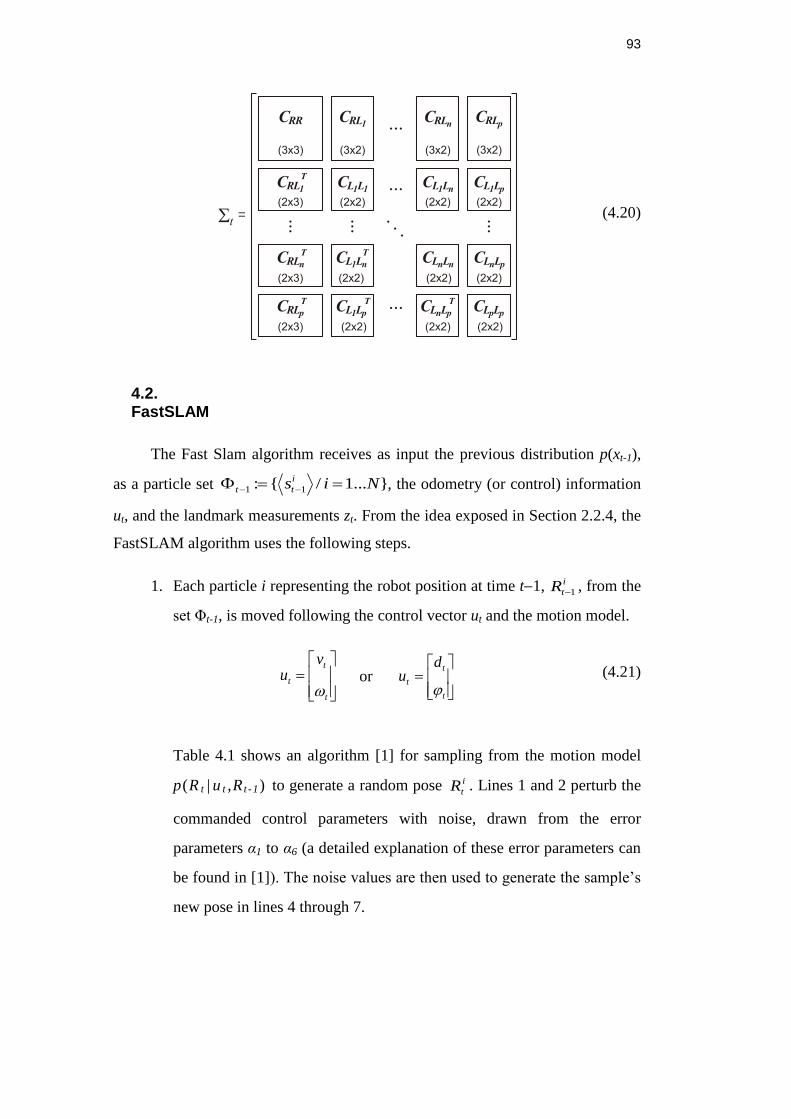
93
(4.20)
4.2. FastSLAM
The Fast Slam algorithm receives as input the previous distribution p(xt-1),
as a particle set }...1/{: 11 Nisi
tt , the odometry (or control) information
ut, and the landmark measurements zt. From the idea exposed in Section 2.2.4, the
FastSLAM algorithm uses the following steps.
1. Each particle i representing the robot position at time t1, i
tR 1 , from the
set Φt-1, is moved following the control vector ut and the motion model.
t
t
t
vu
or
t
t
t
du
(4.21)
Table 4.1 shows an algorithm [1] for sampling from the motion model
p(R t | u t ,R t -1) to generate a random pose i
tR . Lines 1 and 2 perturb the
commanded control parameters with noise, drawn from the error
parameters α1 to α6 (a detailed explanation of these error parameters can
be found in [1]). The noise values are then used to generate the sample’s
new pose in lines 4 through 7.
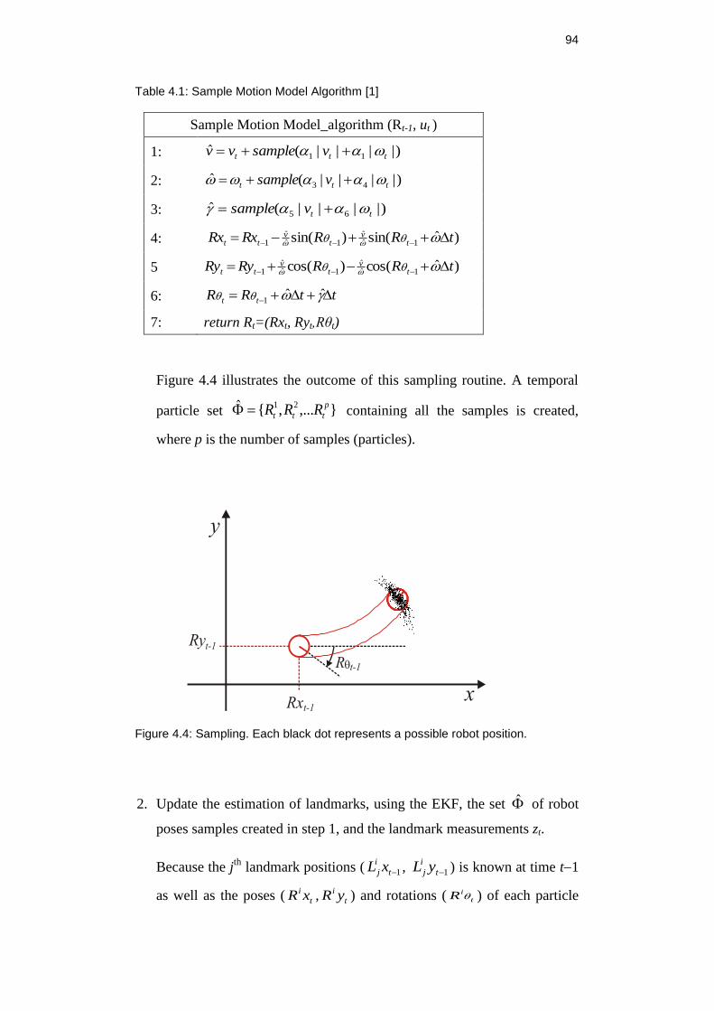
94
Table 4.1: Sample Motion Model Algorithm [1]
Sample Motion Model_algorithm (Rt-1, ut )
1: )||||(ˆ11 ttt vsamplevv
2: )||||(ˆ43 ttt vsample
3: )||||(ˆ65 ttvsample
4: )ˆsin()sin( 1ˆˆ
1ˆˆ
1 tRRRxRx tv
tv
tt
5 )ˆcos()cos( 1ˆˆ
1ˆˆ
1 tRRRyRy tv
tv
tt
6: ttRR tt ˆˆ1
7: return Rt=(Rxt, Ryt,Rθt)
Figure 4.4 illustrates the outcome of this sampling routine. A temporal
particle set },...,{ˆ 21 p
ttt RRR containing all the samples is created,
where p is the number of samples (particles).
Figure 4.4: Sampling. Each black dot represents a possible robot position.
2. Update the estimation of landmarks, using the EKF, the set of robot
poses samples created in step 1, and the landmark measurements zt.
Because the jth
landmark positions ( 1t
i
j xL , 1t
i
j yL ) is known at time t1
as well as the poses ( t
i xR , t
i yR ) and rotations ( t
iR ) of each particle
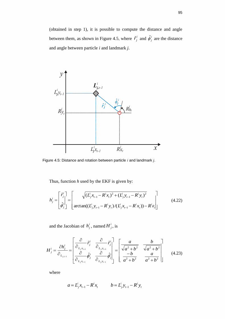
95
(obtained in step 1), it is possible to compute the distance and angle
between them, as shown in Figure 4.5, where i
jr and
i
j are the distance
and angle between particle i and landmark j.
Figure 4.5: Distance and rotation between particle i and landmark j.
Thus, function h used by the EKF is given by:
t
i
t
i
t
i
jt
i
t
i
j
t
i
t
i
jt
i
t
i
j
i
j
i
ji
j
RxRxLyRyL
yRyLxRxLr
h
))/()arctan((
)()(
ˆ
ˆ
11
2
1
2
1
(4.22)
and the Jacobian of i
jh , namedi
jH , is
2222
2222
ˆˆ
ˆˆ
11
11
1,
ba
a
ba
bba
b
ba
arrh
Hi
j
yL
i
j
xL
i
j
yL
i
j
xL
L
i
ji
j
tjtj
tjtj
tj
(4.23)
where
t
i
t
i
jt
i
t
i
j yRyLbxRxLa 11
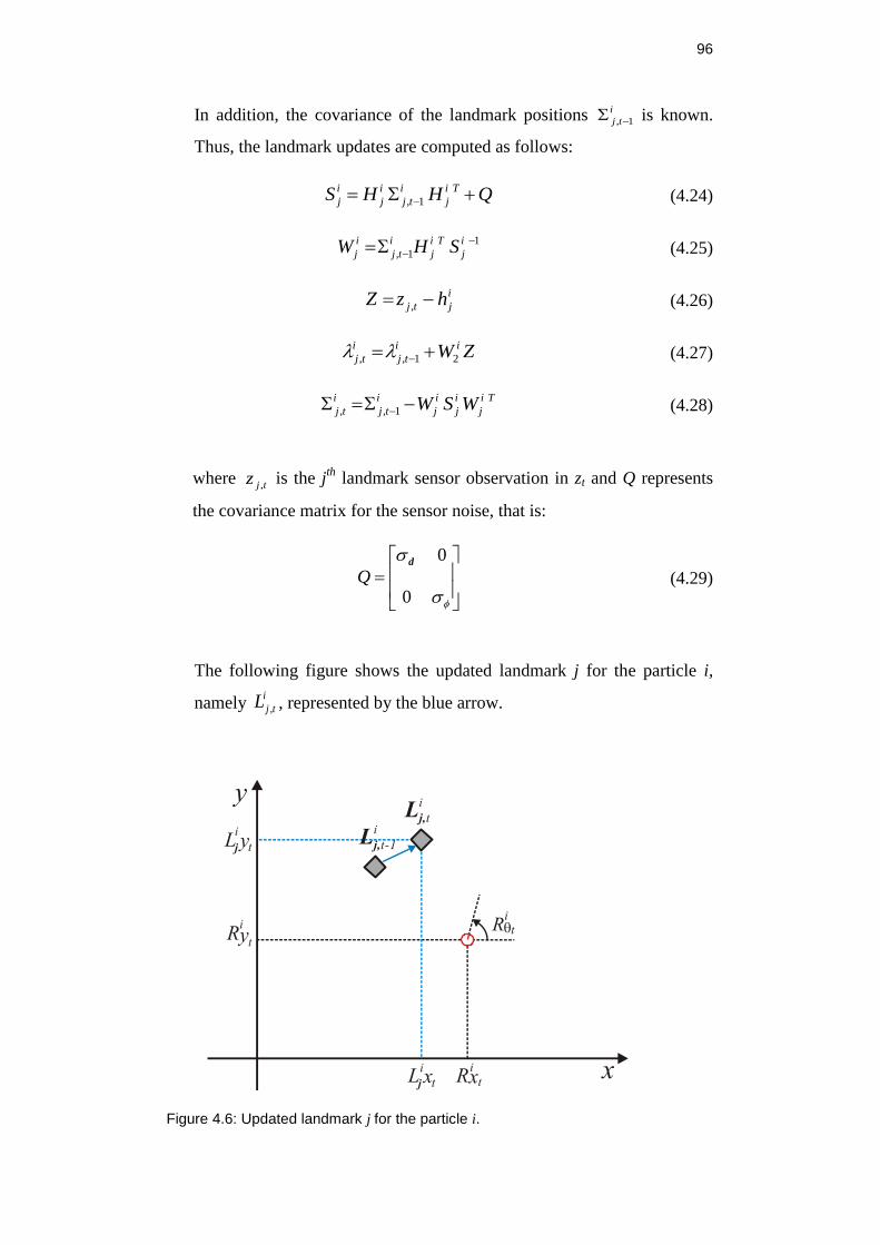
96
In addition, the covariance of the landmark positions i
tj 1, is known.
Thus, the landmark updates are computed as follows:
QHHS Ti
j
i
tj
i
j
i
j 1, (4.24)
1
1,
i
j
Ti
j
i
tj
i
j SHW
(4.25)
i
jtj hzZ ,
(4.26)
ZW ii
tj
i
tj 21,,
(4.27)
Ti
j
i
j
i
j
i
tj
i
tj WSW 1,,
(4.28)
where tjz , is the jth
landmark sensor observation in zt and Q represents
the covariance matrix for the sensor noise, that is:
0
0d
Q
(4.29)
The following figure shows the updated landmark j for the particle i,
namely i
tjL , , represented by the blue arrow.
Figure 4.6: Updated landmark j for the particle i.
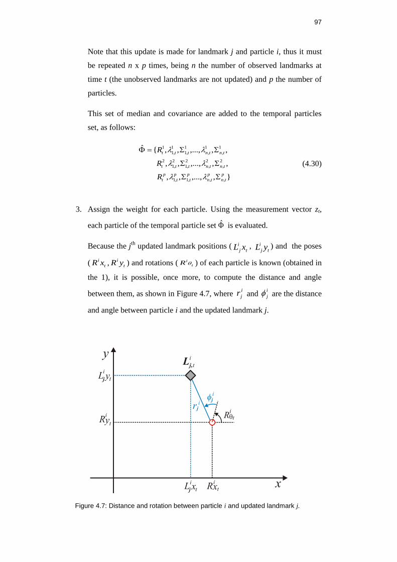
97
Note that this update is made for landmark j and particle i, thus it must
be repeated n x p times, being n the number of observed landmarks at
time t (the unobserved landmarks are not updated) and p the number of
particles.
This set of median and covariance are added to the temporal particles
set, as follows:
},,...,,,
,,,...,,,
,,,...,,,{ˆ
,,,1,1
2
,
2
,
2
,1
2
,1
2
1
,
1
,
1
,1
1
,1
1
p
tn
p
tn
p
t
p
t
p
t
tntnttt
tntnttt
R
R
R
(4.30)
3. Assign the weight for each particle. Using the measurement vector zt,
each particle of the temporal particle set is evaluated.
Because the jth
updated landmark positions (t
i
j xL , t
i
j yL ) and the poses
( t
i xR , t
i yR ) and rotations ( t
iR ) of each particle is known (obtained in
the 1), it is possible, once more, to compute the distance and angle
between them, as shown in Figure 4.7, where i
jr and
i
j are the distance
and angle between particle i and the updated landmark j.
Figure 4.7: Distance and rotation between particle i and updated landmark j.
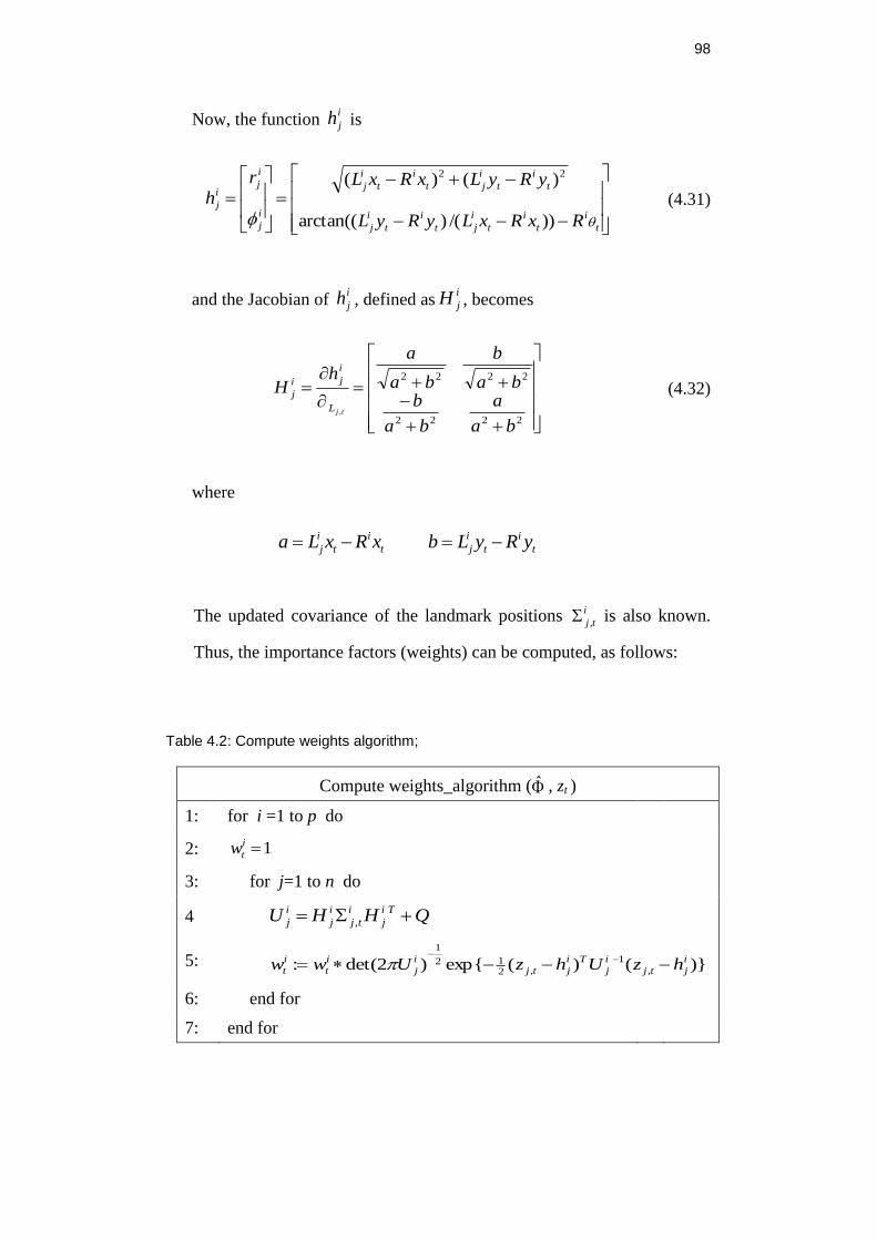
98
Now, the function i
jh is
t
i
t
i
t
i
jt
i
t
i
j
t
i
t
i
jt
i
t
i
j
i
j
i
ji
j
RxRxLyRyL
yRyLxRxLr
h
))/()arctan((
)()( 22
(4.31)
and the Jacobian of i
jh , defined asi
jH , becomes
2222
2222
,
ba
a
ba
bba
b
ba
ah
H
tjL
i
ji
j (4.32)
where
t
i
t
i
jt
i
t
i
j yRyLbxRxLa
The updated covariance of the landmark positions i
tj , is also known.
Thus, the importance factors (weights) can be computed, as follows:
Table 4.2: Compute weights algorithm;
Compute weights_algorithm ( , zt )
1: for i =1 to p do
2: 1i
tw
3: for j=1 to n do
4
QHHU Ti
j
i
tj
i
j
i
j ,
5:
)}()(exp{)2det(: ,
1
,212
1
i
jtj
i
j
Ti
jtj
i
j
i
t
i
t hzUhzUww
6: end for
7: end for
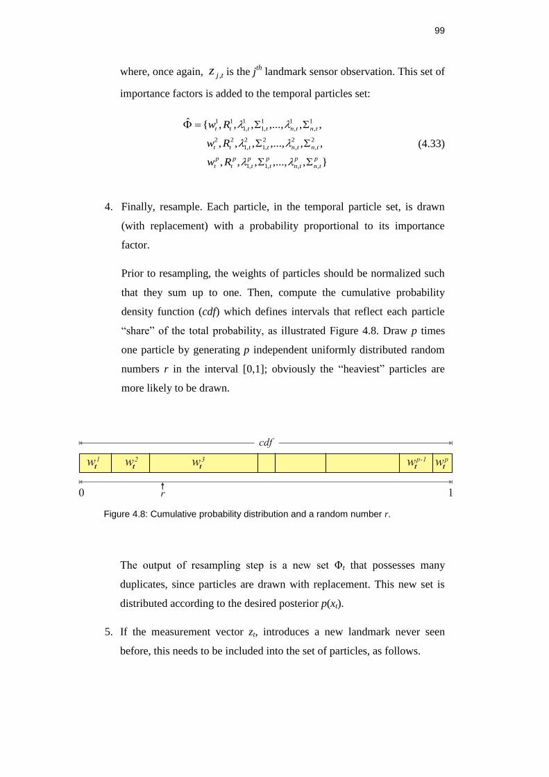
99
where, once again, tjz , is the jth
landmark sensor observation. This set of
importance factors is added to the temporal particles set:
},,...,,,,
,,,...,,,,
,,,...,,,,{ˆ
,,,1,1
2
,
2
,
2
,1
2
,1
22
1
,
1
,
1
,1
1
,1
11
p
tn
p
tn
p
t
p
t
p
t
p
t
tntntttt
tntntttt
Rw
Rw
Rw
(4.33)
4. Finally, resample. Each particle, in the temporal particle set, is drawn
(with replacement) with a probability proportional to its importance
factor.
Prior to resampling, the weights of particles should be normalized such
that they sum up to one. Then, compute the cumulative probability
density function (cdf) which defines intervals that reflect each particle
“share” of the total probability, as illustrated Figure 4.8. Draw p times
one particle by generating p independent uniformly distributed random
numbers r in the interval [0,1]; obviously the “heaviest” particles are
more likely to be drawn.
Figure 4.8: Cumulative probability distribution and a random number r.
The output of resampling step is a new set Φt that possesses many
duplicates, since particles are drawn with replacement. This new set is
distributed according to the desired posterior p(xt).
5. If the measurement vector zt, introduces a new landmark never seen
before, this needs to be included into the set of particles, as follows.
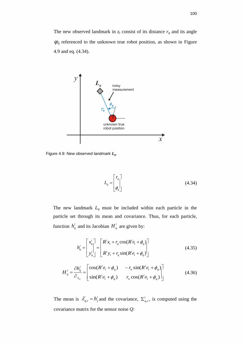
100
The new observed landmark in zt consist of its distance rq and its angle
ϕq referenced to the unknown true robot position, as shown in Figure
4.9 and eq. (4.34).
Figure 4.9: New observed landmark Lq.
q
q
q
r
L
(4.34)
The new landmark Lq must be included within each particle in the
particle set through its mean and covariance. Thus, for each particle,
function i
qh and its Jacobian i
qH are given by:
)sin(
)cos(
qt
i
qt
i
qt
i
qt
i
i
q
i
qi
q
RryR
RrxR
y
x
h
(4.35)
)cos()sin(
)sin()cos(
qt
i
nqt
i
qt
i
nqt
i
L
i
qi
q
RrR
RrRhH
q
(4.36)
The mean is
i
j
i
tq h, and the covariance, i
tq, , is computed using the
covariance matrix for the sensor noise Q:
101
Ti
q
i
q
i
tq HQH ,
(4.37)
Now the particle set Φt has a new landmark incorporated, making the
number of total landmarks become n:=n+1.
4.3. Simulator
To test the grid mapping algorithm, it is necessary to acquire data from a
LRF mounted on a robot that moves along a structured environment. It is also
possible to evaluate the algorithm from simulations of both the environment and
the LRF readings, as long as noise is introduced in the process.
The simulation of the robot perception based on LRF provides several
advantages. First of all, it is cheaper than experimenting with a real device. The
simulator gives the opportunity to concentrate more on the intelligence algorithms
such as localization and mapping (SLAM). Developing the simulator is easier
than building a new robot or perception system [29], due to the testability of many
configurations.
The simulator used in this work is implemented on Matlab®, explaining as
follows.
4.3.1. 3D Environment Simulation
The element used in the simulator to represent the structured environment is
the plane. All structured environment elements are approximated using planes;
straight walls, curved walls, doors, windows, floors, ceilings, etc, can be modeled
using a group of rectangles. Figure 4.10 shows an environment constructed in
such a way.
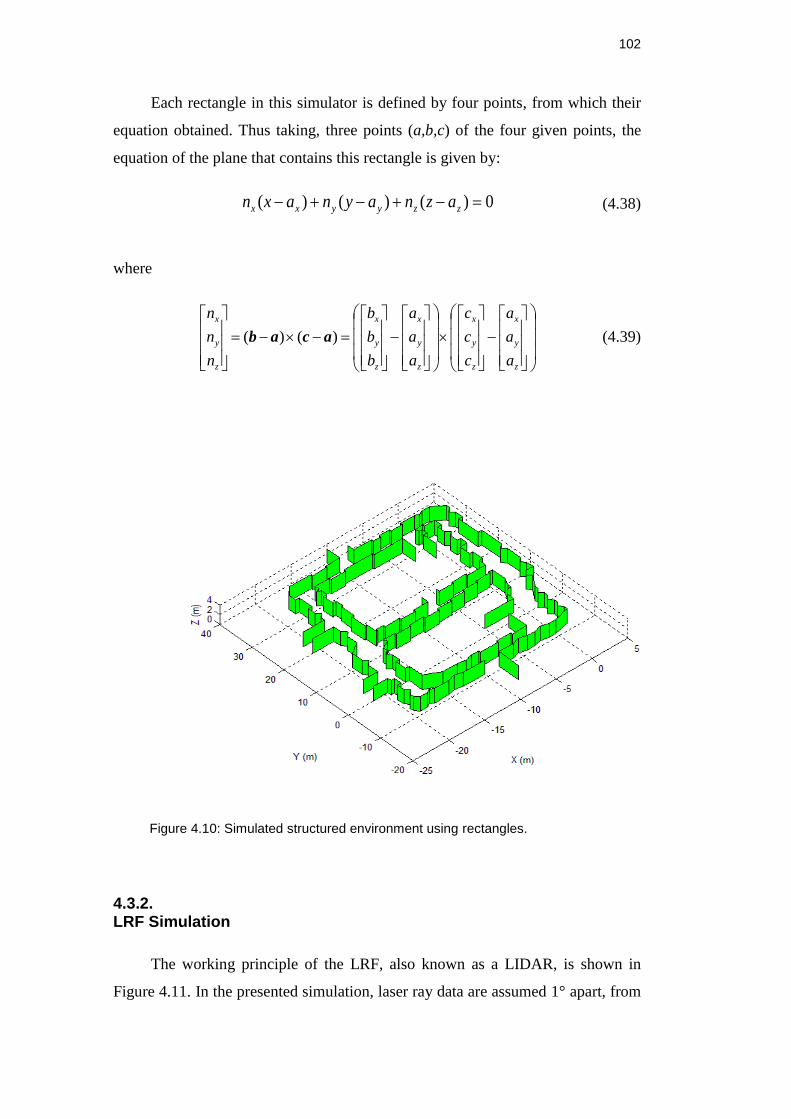
102
Each rectangle in this simulator is defined by four points, from which their
equation obtained. Thus taking, three points (a,b,c) of the four given points, the
equation of the plane that contains this rectangle is given by:
0)()()( zzyyxx aznaynaxn (4.38)
where
z
y
x
z
y
x
z
y
x
z
y
x
z
y
x
a
a
a
c
c
c
a
a
a
b
b
b
n
n
n
)()( acab (4.39)
Figure 4.10: Simulated structured environment using rectangles.
4.3.2. LRF Simulation
The working principle of the LRF, also known as a LIDAR, is shown in
Figure 4.11. In the presented simulation, laser ray data are assumed 1° apart, from
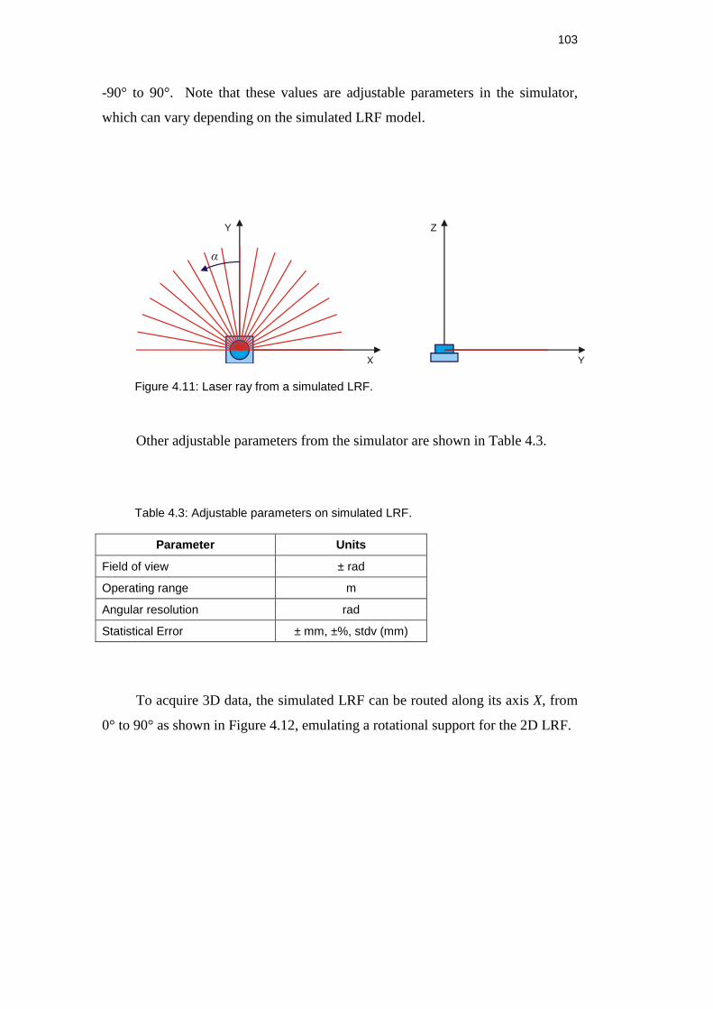
103
-90° to 90°. Note that these values are adjustable parameters in the simulator,
which can vary depending on the simulated LRF model.
Figure 4.11: Laser ray from a simulated LRF.
Other adjustable parameters from the simulator are shown in Table 4.3.
Table 4.3: Adjustable parameters on simulated LRF.
Parameter Units
Field of view ± rad
Operating range m
Angular resolution rad
Statistical Error ± mm, ±%, stdv (mm)
To acquire 3D data, the simulated LRF can be routed along its axis X, from
0° to 90° as shown in Figure 4.12, emulating a rotational support for the 2D LRF.
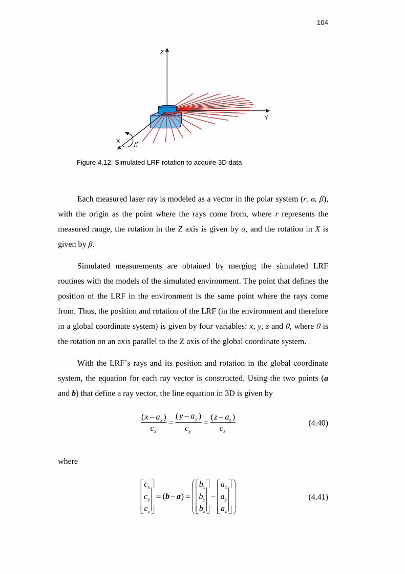
104
Figure 4.12: Simulated LRF rotation to acquire 3D data
Each measured laser ray is modeled as a vector in the polar system (r, α, β),
with the origin as the point where the rays come from, where r represents the
measured range, the rotation in the Z axis is given by α, and the rotation in X is
given by β.
Simulated measurements are obtained by merging the simulated LRF
routines with the models of the simulated environment. The point that defines the
position of the LRF in the environment is the same point where the rays come
from. Thus, the position and rotation of the LRF (in the environment and therefore
in a global coordinate system) is given by four variables: x, y, z and θ, where θ is
the rotation on an axis parallel to the Z axis of the global coordinate system.
With the LRF’s rays and its position and rotation in the global coordinate
system, the equation for each ray vector is constructed. Using the two points (a
and b) that define a ray vector, the line equation in 3D is given by
z
z
y
y
x
x
c
az
c
ay
c
ax )()()(
(4.40)
where
z
y
x
z
y
x
z
y
x
a
a
a
b
b
b
c
c
c
)( ab (4.41)
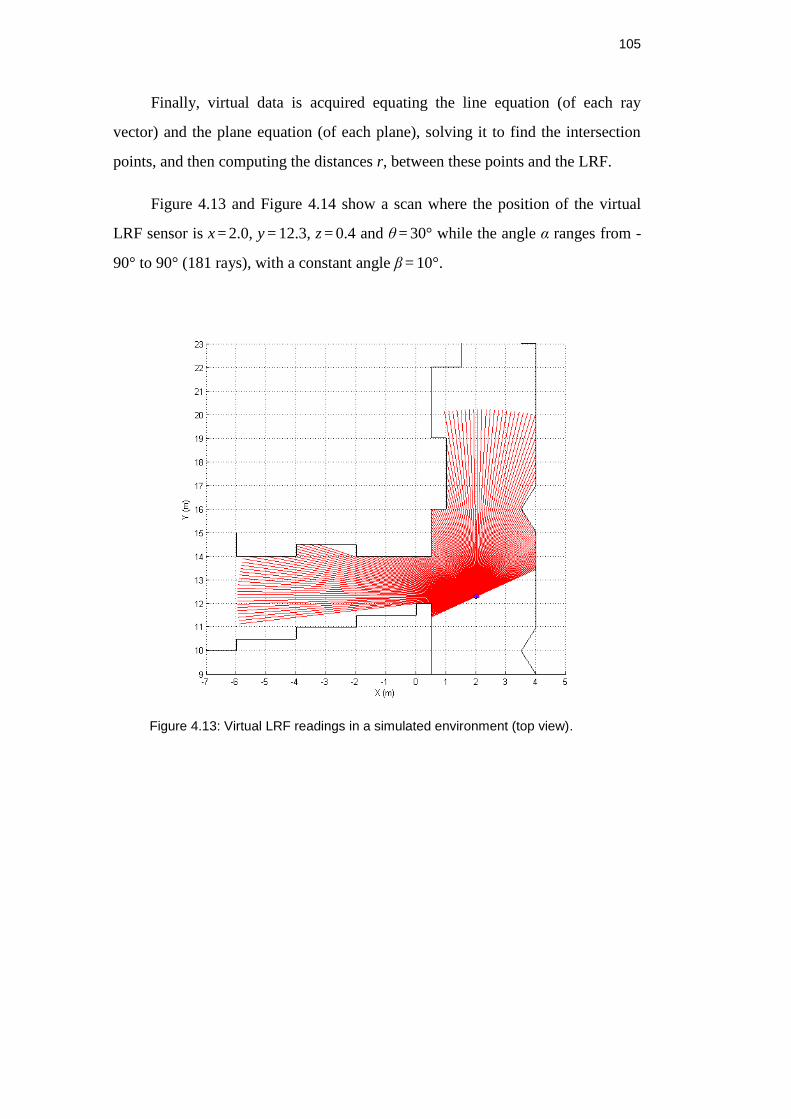
105
Finally, virtual data is acquired equating the line equation (of each ray
vector) and the plane equation (of each plane), solving it to find the intersection
points, and then computing the distances r, between these points and the LRF.
Figure 4.13 and Figure 4.14 show a scan where the position of the virtual
LRF sensor is x = 2.0, y = 12.3, z = 0.4 and θ = 30° while the angle α ranges from -
90° to 90° (181 rays), with a constant angle β = 10°.
Figure 4.13: Virtual LRF readings in a simulated environment (top view).
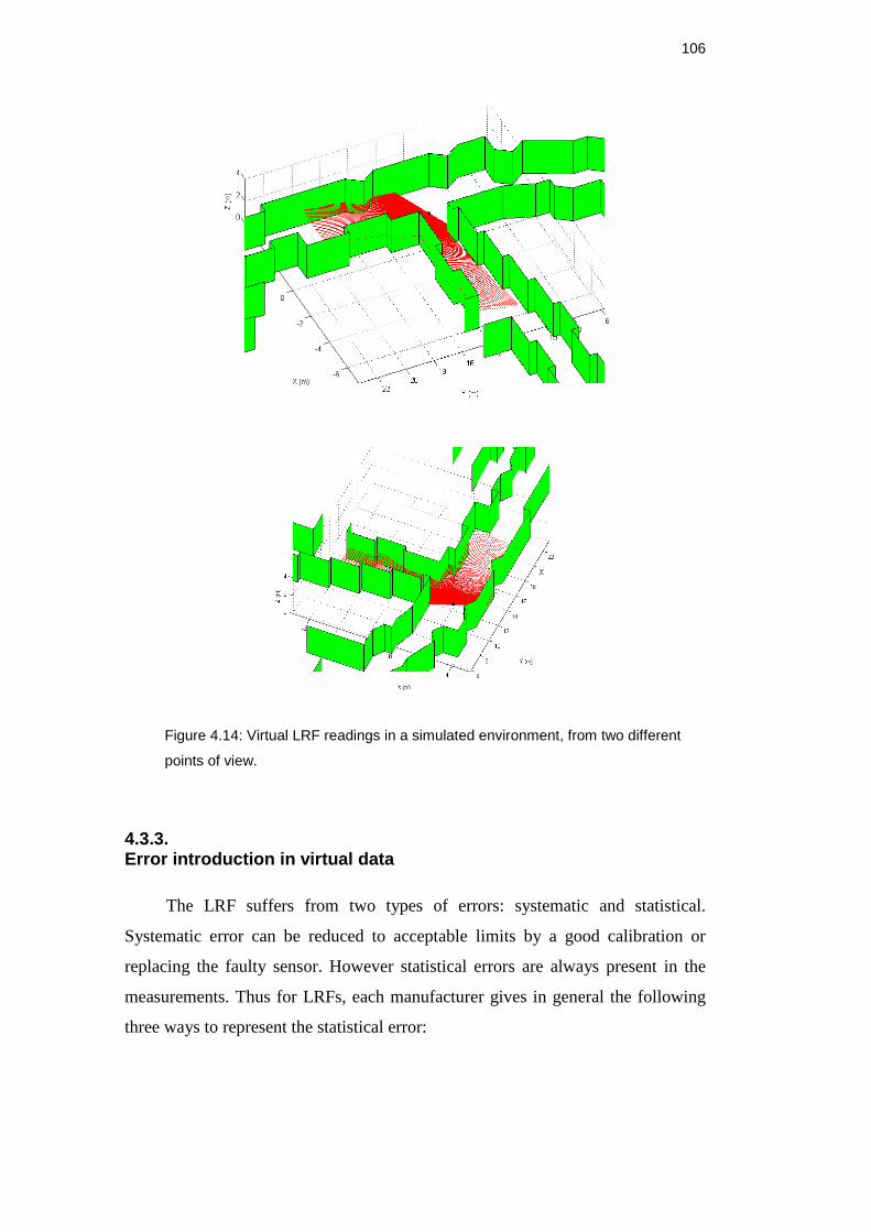
106
Figure 4.14: Virtual LRF readings in a simulated environment, from two different
points of view.
4.3.3. Error introduction in virtual data
The LRF suffers from two types of errors: systematic and statistical.
Systematic error can be reduced to acceptable limits by a good calibration or
replacing the faulty sensor. However statistical errors are always present in the
measurements. Thus for LRFs, each manufacturer gives in general the following
three ways to represent the statistical error:
107
By standard deviation. The standard deviations (stdv) of the
measurements are given. For example the LRF SICK, model LMS200,
has a stdv of 5mm, and the model LMS291 has a stdv of 10mm.
By a percentage of the measurement or by a fixed number. For
instance, the LRF SICK, model LMS291-S05 has an error of +/- 10mm.
By a fixed number until a certain range, and beyond that by a
percentage. For instance, the LRF HOKUYO, model URG-04LX, has an
error of +/- 10mm in the range from 0 to 1m and, beyond that, 1% of the
measurement. The model URG-04LX-UG01 has an error of +/- 30mm in
the range from 0 to 1m and beyond that, 3% of the measurement.
These ways of expressing the error can be simulated and introduced in the
distances r, virtually measured from the presented simulator.
The above presented simulator description just focused in its basic
functionalities, however there are innumerable improvements that can be made,
especially regarding the performance in time response. Solving equations for
many planes/rectangles and lines is computationally expensive. Reference [30] a
simulated 3D laser measurement system is presented, based on LMS SICK 200
mounted on a rotational platform. This simulator uses multi core processing
power to generate 3D data. In [31] a simulator for airborne altimetric LIDAR is
presented. This simulator is conceived having three components: terrain
component, sensor component and platform component.
4.4. Scan Matching
One of the objectives of this work is to map an environment without using
odometry information. Thus, the unique available information is taken from the
scans made by the Laser Range Finder (LRF). To estimate the robot movement,
the alignment of two consecutive scans needs to be performed.
It is important to notice that the scan matching searches for the displacement
between two consecutive scans, but this displacement is not necessarily the robot
108
displacement, since LRF may be mounted away from the robot center. To
calculate the robot movement it is necessary to know where the LRF is situated on
the robot, specifically where the LRF is located with respect to the coordinate
system of the robot.
As described in Section 2.3.3, the scan matching method used in this work
is the Normal Distribution Transform (NDT). This method was selected basically
because it has a featureless representation of the environment, consequently it
doesn’t need search for correspondences in the scans.
NDT uses Newton´s algorithm to minimize the function f = score. In most
systems, the initial estimate of the solution is given by odometry information. But
large error in the initial position estimate can contribute to the non-convergence of
the algorithm.
Therefore, to generate a robust algorithm, in this work a Genetic Algorithm
(GA) is used for optimization, from the Differential Evolution routines described
in Section 2.4.5.
4.4.1. Differential Evolution Optimization for NDT
First, let’s rewrite eq. (2.15)
i
iiii qxqxscore
2
)(Σ)(exp)(
1
i
T
p (4.42)
The outline of this optimization, given two scans (the first and the second
one), is as follows:
1. Build the NDT of the first scan, as described in Section 2.3.3.
2. Use the first scan to evaluate the distribution of its points using eq.
(4.42). This means that the vector of parameters must be p =[0 0 0]T and
the score(p) will give a value that is the maximum possible. This is,
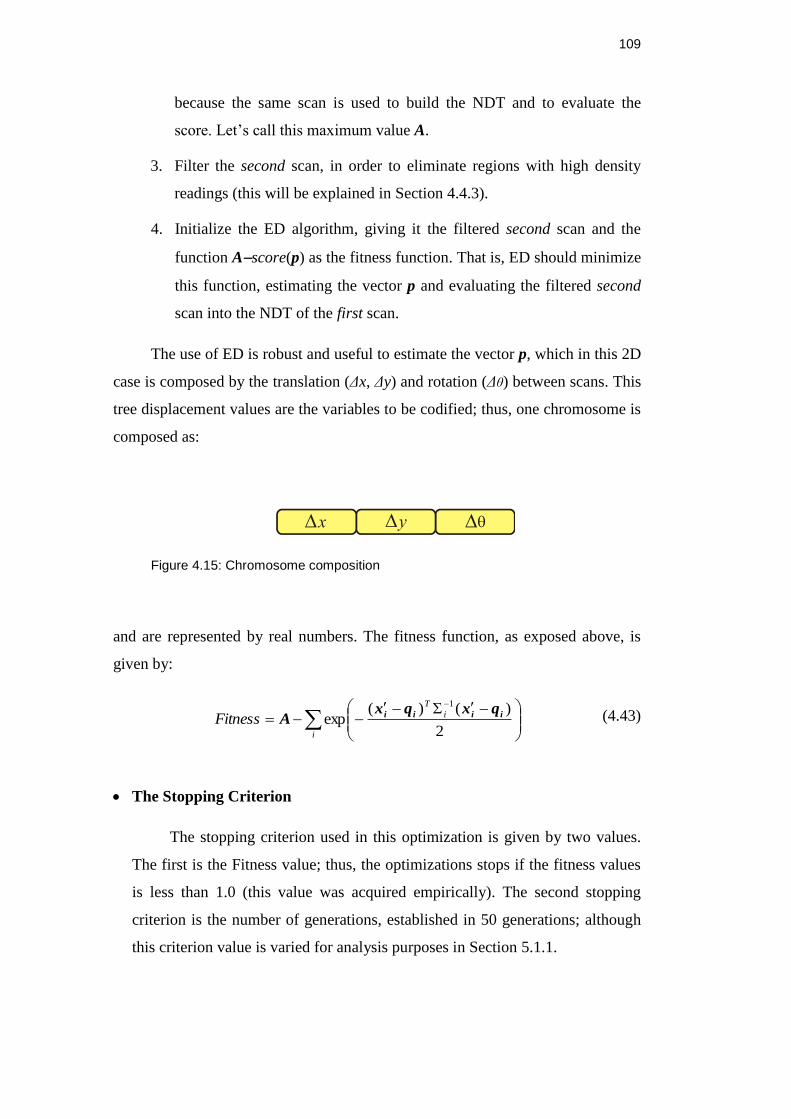
109
because the same scan is used to build the NDT and to evaluate the
score. Let’s call this maximum value A.
3. Filter the second scan, in order to eliminate regions with high density
readings (this will be explained in Section 4.4.3).
4. Initialize the ED algorithm, giving it the filtered second scan and the
function Ascore(p) as the fitness function. That is, ED should minimize
this function, estimating the vector p and evaluating the filtered second
scan into the NDT of the first scan.
The use of ED is robust and useful to estimate the vector p, which in this 2D
case is composed by the translation (Δx, Δy) and rotation (Δθ) between scans. This
tree displacement values are the variables to be codified; thus, one chromosome is
composed as:
Figure 4.15: Chromosome composition
and are represented by real numbers. The fitness function, as exposed above, is
given by:
i
i
T
Fitness2
)()(exp
1
iiii qxqxA (4.43)
The Stopping Criterion
The stopping criterion used in this optimization is given by two values.
The first is the Fitness value; thus, the optimizations stops if the fitness values
is less than 1.0 (this value was acquired empirically). The second stopping
criterion is the number of generations, established in 50 generations; although
this criterion value is varied for analysis purposes in Section 5.1.1.
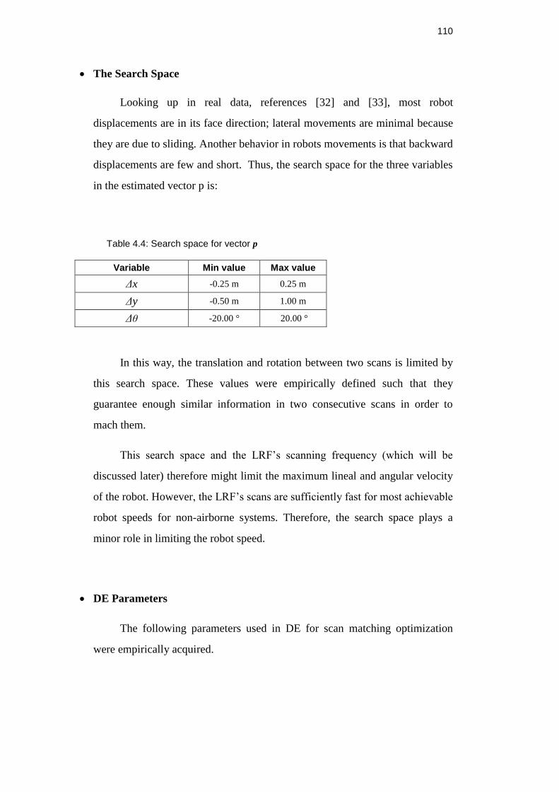
110
The Search Space
Looking up in real data, references [32] and [33], most robot
displacements are in its face direction; lateral movements are minimal because
they are due to sliding. Another behavior in robots movements is that backward
displacements are few and short. Thus, the search space for the three variables
in the estimated vector p is:
Table 4.4: Search space for vector p
Variable Min value Max value
Δx -0.25 m 0.25 m
Δy -0.50 m 1.00 m
Δθ -20.00 ° 20.00 °
In this way, the translation and rotation between two scans is limited by
this search space. These values were empirically defined such that they
guarantee enough similar information in two consecutive scans in order to
mach them.
This search space and the LRF’s scanning frequency (which will be
discussed later) therefore might limit the maximum lineal and angular velocity
of the robot. However, the LRF’s scans are sufficiently fast for most achievable
robot speeds for non-airborne systems. Therefore, the search space plays a
minor role in limiting the robot speed.
DE Parameters
The following parameters used in DE for scan matching optimization
were empirically acquired.
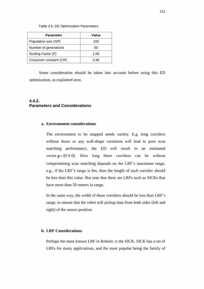
111
Table 4.5: DE Optimization Parameters.
Parameter Value
Population size (NP) 100
Number of generations 50
Scaling Factor (F) 1.00
Crossover constant (CR) 0.95
Some consideration should be taken into account before using this ED
optimization, as explained next.
4.4.2. Parameters and Considerations
a. Environment considerations
The environment to be mapped needs variety. E.g. long corridors
without doors or any wall-shape variations will lead to poor scan
matching performance, the ED will result in an estimated
vector [0 0 0]p . How long these corridors can be without
compromising scan matching depends on the LRF’s maximum range,
e.g., if the LRF’s range is 8m, then the length of such corridor should
be less than this value. But note that there are LRFs such as SICKs that
have more than 50 meters in range.
In the same way, the width of these corridors should be less than LRF’s
range, to ensure that the robot will pickup data from both sides (left and
right) of the sensor position.
b. LRF Considerations
Perhaps the most known LRF in Robotic is the SICK. SICK has a set of
LRFs for many applications, and the most popular being the family of
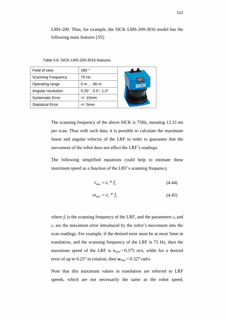
112
LMS-200. Thus, for example, the SICK LMS-200-3016 model has the
following main features [35]:
Table 4.6: SICK LMS-200-3016 features.
Field of view 180 °
Scanning Frequency 75 Hz
Operating range 0 m … 80 m
Angular resolution 0.25° , 0.5°, 1.0°
Systematic Error +/- 15mm
Statistical Error +/- 5mm
The scanning frequency of the above SICK is 75Hz, meaning 13.33 ms
per scan. Thus with such data, it is possible to calculate the maximum
linear and angular velocity of the LRF in order to guarantee that the
movement of the robot does not affect the LRF’s readings.
The following simplified equations could help to estimate these
maximum speed as a function of the LRF’s scanning frequency.
st fv *max (4.44)
sr f*max (4.45)
where fs is the scanning frequency of the LRF, and the parameters εt and
εr are the maximum error introduced by the robot’s movement into the
scan readings. For example, if the desired error must be at most 5mm in
translation, and the scanning frequency of the LRF is 75 Hz, then the
maximum speed of the LRF is vmax = 0.375 m/s, while for a desired
error of up to 0.25° in rotation, then wmax = 0.327 rad/s.
Note that this maximum values in translation are referred to LRF
speeds, which are not necessarily the same as the robot speed,
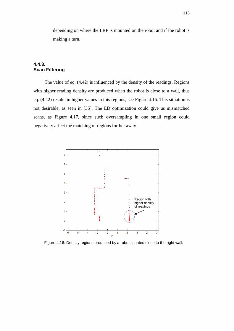
113
depending on where the LRF is mounted on the robot and if the robot is
making a turn.
4.4.3. Scan Filtering
The value of eq. (4.42) is influenced by the density of the readings. Regions
with higher reading density are produced when the robot is close to a wall, thus
eq. (4.42) results in higher values in this regions, see Figure 4.16. This situation is
not desirable, as seen in [35]. The ED optimization could give us mismatched
scans, as Figure 4.17, since such oversampling in one small region could
negatively affect the matching of regions further away.
Figure 4.16: Density regions produced by a robot situated close to the right wall.
Region with higher density of readings
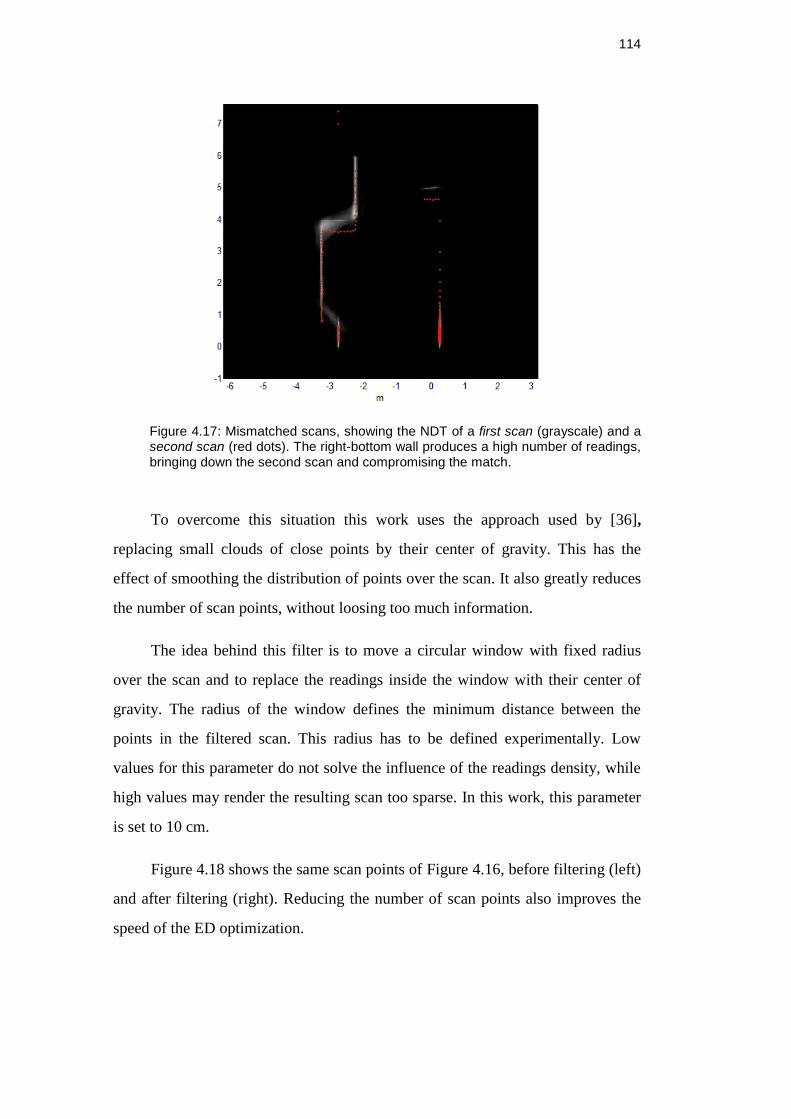
114
Figure 4.17: Mismatched scans, showing the NDT of a first scan (grayscale) and a second scan (red dots). The right-bottom wall produces a high number of readings, bringing down the second scan and compromising the match.
To overcome this situation this work uses the approach used by [36],
replacing small clouds of close points by their center of gravity. This has the
effect of smoothing the distribution of points over the scan. It also greatly reduces
the number of scan points, without loosing too much information.
The idea behind this filter is to move a circular window with fixed radius
over the scan and to replace the readings inside the window with their center of
gravity. The radius of the window defines the minimum distance between the
points in the filtered scan. This radius has to be defined experimentally. Low
values for this parameter do not solve the influence of the readings density, while
high values may render the resulting scan too sparse. In this work, this parameter
is set to 10 cm.
Figure 4.18 shows the same scan points of Figure 4.16, before filtering (left)
and after filtering (right). Reducing the number of scan points also improves the
speed of the ED optimization.
Region with higher density of readings
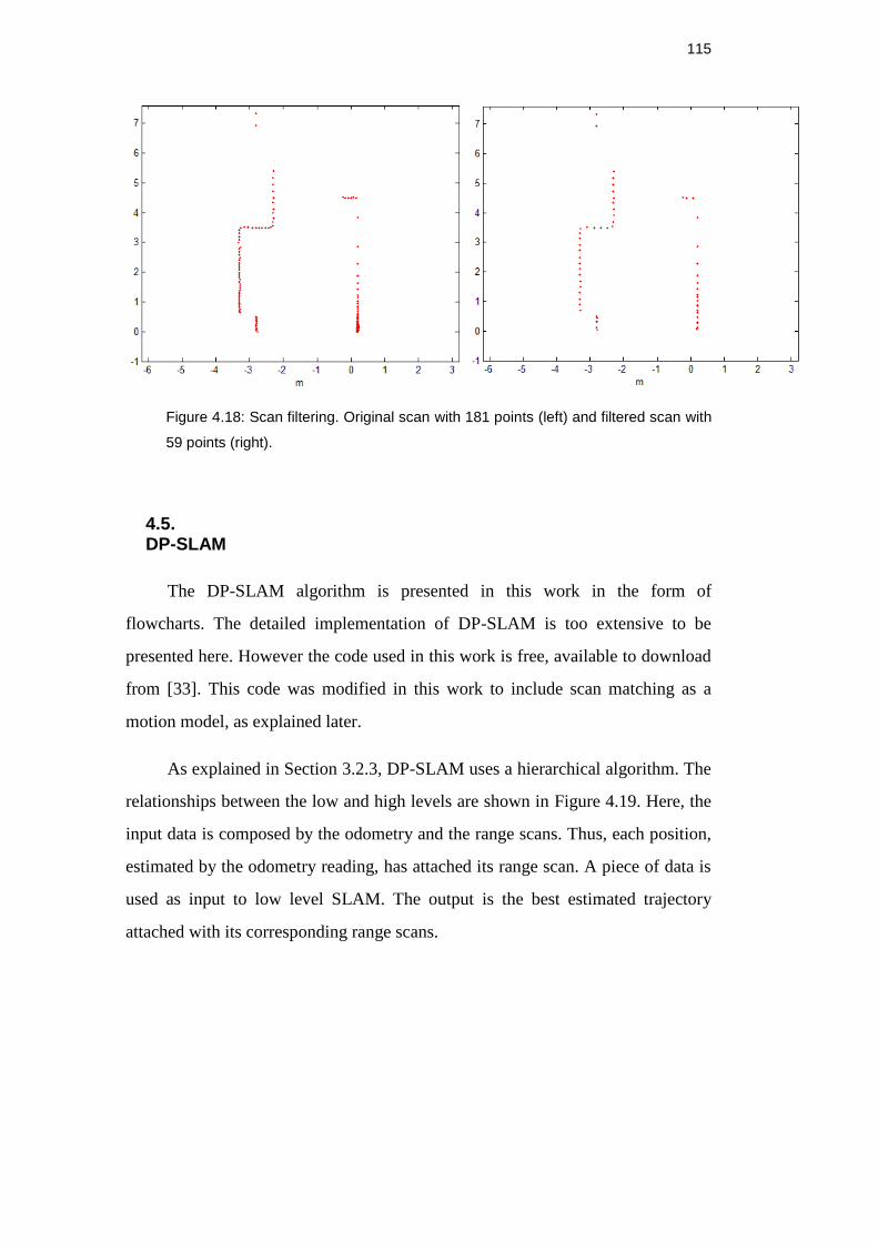
115
Figure 4.18: Scan filtering. Original scan with 181 points (left) and filtered scan with
59 points (right).
4.5. DP-SLAM
The DP-SLAM algorithm is presented in this work in the form of
flowcharts. The detailed implementation of DP-SLAM is too extensive to be
presented here. However the code used in this work is free, available to download
from [33]. This code was modified in this work to include scan matching as a
motion model, as explained later.
As explained in Section 3.2.3, DP-SLAM uses a hierarchical algorithm. The
relationships between the low and high levels are shown in Figure 4.19. Here, the
input data is composed by the odometry and the range scans. Thus, each position,
estimated by the odometry reading, has attached its range scan. A piece of data is
used as input to low level SLAM. The output is the best estimated trajectory
attached with its corresponding range scans.
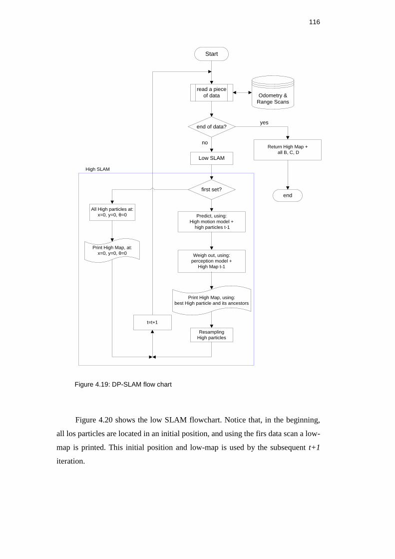
116
Start
Odometry &
Range Scans
end of data?
read a piece
of data
Low SLAM
no
end
yes
first set?
All High particles at:
x=0, y=0, θ=0
Print High Map, at:
x=0, y=0, θ=0
Resampling
High particles
Predict, using:
High motion model +
high particles t-1
Weigh out, using:
perception model +
High Map t-1
t=t+1
Print High Map, using:
best High particle and its ancestors
Return High Map +
all B, C, D
High SLAM
Figure 4.19: DP-SLAM flow chart
Figure 4.20 shows the low SLAM flowchart. Notice that, in the beginning,
all los particles are located in an initial position, and using the firs data scan a low-
map is printed. This initial position and low-map is used by the subsequent t+1
iteration.
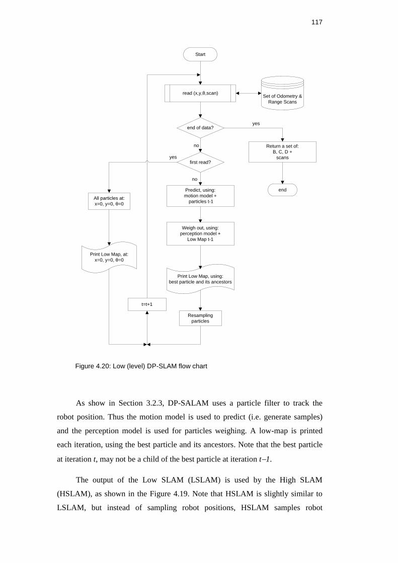
117
Start
end of data?
read (x,y,θ,scan)
Predict, using:
motion model +
particles t-1
Print Low Map, using:
best particle and its ancestors
end
yes
first read?
no
no
Weigh out, using:
perception model +
Low Map t-1
yes
Resampling
particles
Print Low Map, at:
x=0, y=0, θ=0
All particles at:
x=0, y=0, θ=0
t=t+1
Return a set of:
B, C, D +
scans
Set of Odometry &
Range Scans
Figure 4.20: Low (level) DP-SLAM flow chart
As show in Section 3.2.3, DP-SALAM uses a particle filter to track the
robot position. Thus the motion model is used to predict (i.e. generate samples)
and the perception model is used for particles weighing. A low-map is printed
each iteration, using the best particle and its ancestors. Note that the best particle
at iteration t, may not be a child of the best particle at iteration t1.
The output of the Low SLAM (LSLAM) is used by the High SLAM
(HSLAM), as shown in the Figure 4.19. Note that HSLAM is slightly similar to
LSLAM, but instead of sampling robot positions, HSLAM samples robot
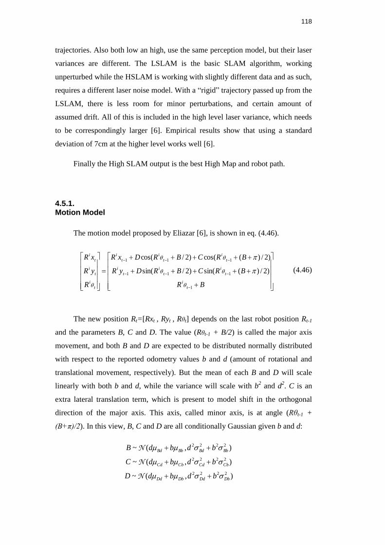
118
trajectories. Also both low an high, use the same perception model, but their laser
variances are different. The LSLAM is the basic SLAM algorithm, working
unperturbed while the HSLAM is working with slightly different data and as such,
requires a different laser noise model. With a “rigid” trajectory passed up from the
LSLAM, there is less room for minor perturbations, and certain amount of
assumed drift. All of this is included in the high level laser variance, which needs
to be correspondingly larger [6]. Empirical results show that using a standard
deviation of 7cm at the higher level works well [6].
Finally the High SLAM output is the best High Map and robot path.
4.5.1. Motion Model
The motion model proposed by Eliazar [6], is shown in eq. (4.46).
BR
BRCBRDyR
BRCBRDxR
R
yR
xR
t
i
t
i
t
i
t
i
t
i
t
i
t
i
t
i
t
i
t
i
1
111
111
)2/)(sin()2/sin(
)2/)(cos()2/cos(
(4.46)
The new position Rt=[Rxt , Ryt , Rθt] depends on the last robot position Rt-1
and the parameters B, C and D. The value (Rθt-1 + B/2) is called the major axis
movement, and both B and D are expected to be distributed normally distributed
with respect to the reported odometry values b and d (amount of rotational and
translational movement, respectively). But the mean of each B and D will scale
linearly with both b and d, while the variance will scale with b2 and d
2. C is an
extra lateral translation term, which is present to model shift in the orthogonal
direction of the major axis. This axis, called minor axis, is at angle (Rθt-1 +
(B+π)/2). In this view, B, C and D are all conditionally Gaussian given b and d:
),(~
),(~
),(~
2222
2222
2222
DbDdDbDd
CbCdCbCd
BbBdBbBd
bdbdD
bdbdC
bdbdB
Ν
Ν
Ν
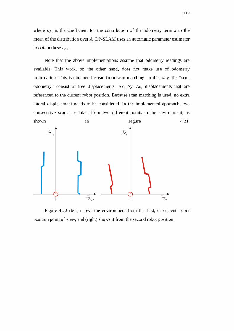
119
where μAx is the coefficient for the contribution of the odometry term x to the
mean of the distribution over A. DP-SLAM uses an automatic parameter estimator
to obtain these μAx.
Note that the above implementations assume that odometry readings are
available. This work, on the other hand, does not make use of odometry
information. This is obtained instead from scan matching. In this way, the “scan
odometry” consist of tree displacements: Δx, Δy, Δθ, displacements that are
referenced to the current robot position. Because scan matching is used, no extra
lateral displacement needs to be considered. In the implemented approach, two
consecutive scans are taken from two different points in the environment, as
shown in Figure 4.21.
Figure 4.22 (left) shows the environment from the first, or current, robot
position point of view, and (right) shows it from the second robot position.
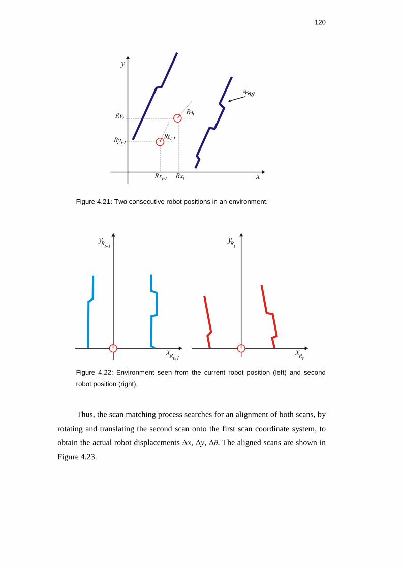
120
Figure 4.21: Two consecutive robot positions in an environment.
Figure 4.22: Environment seen from the current robot position (left) and second
robot position (right).
Thus, the scan matching process searches for an alignment of both scans, by
rotating and translating the second scan onto the first scan coordinate system, to
obtain the actual robot displacements Δx, Δy, Δθ. The aligned scans are shown in
Figure 4.23.
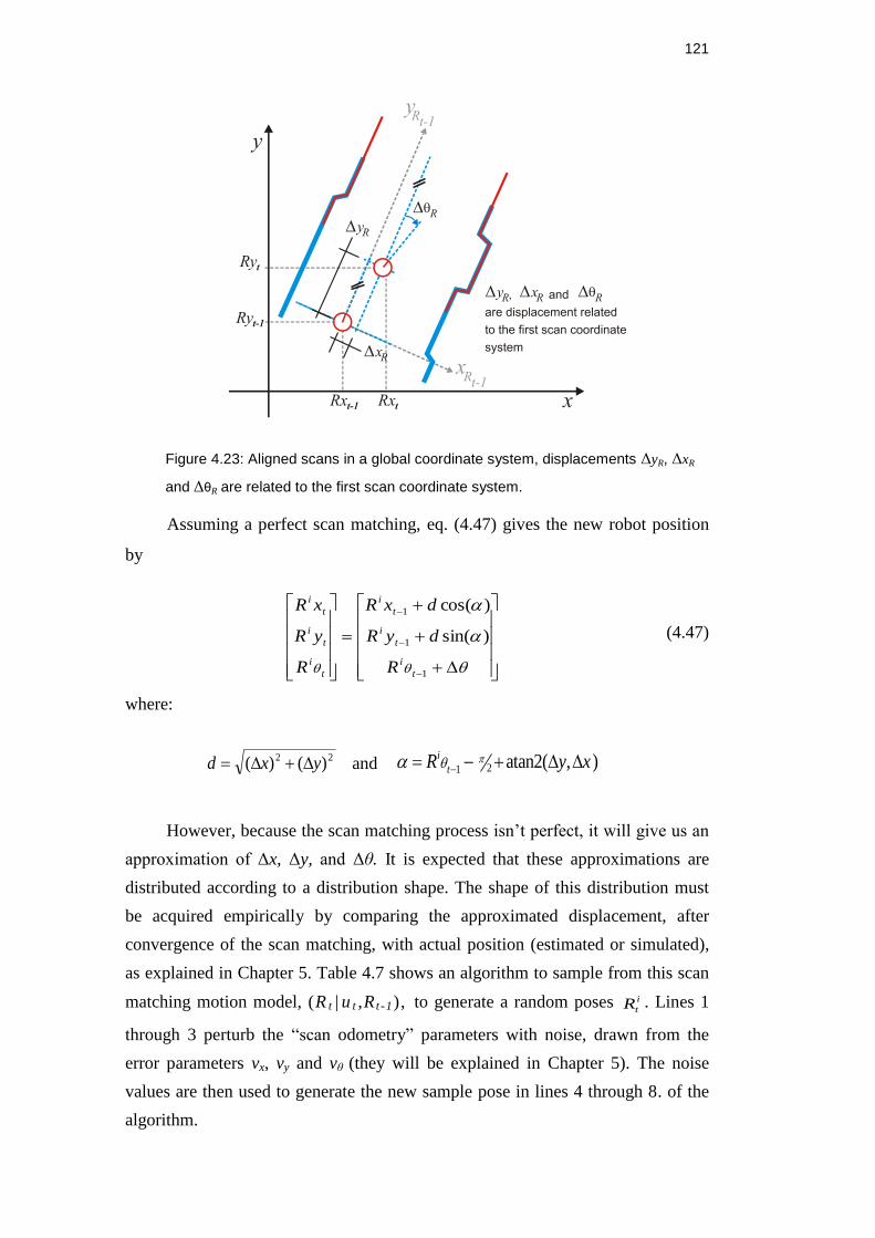
121
Figure 4.23: Aligned scans in a global coordinate system, displacements ΔyR, ΔxR
and ΔθR are related to the first scan coordinate system.
Assuming a perfect scan matching, eq. (4.47) gives the new robot position
by
1
1
1
)sin(
)cos(
t
i
t
i
t
i
t
i
t
i
t
i
R
dyR
dxR
R
yR
xR
(4.47)
where:
22 )()( yxd
and 21 atan2( , )i
tR y x
However, because the scan matching process isn’t perfect, it will give us an
approximation of Δx, Δy, and Δθ. It is expected that these approximations are
distributed according to a distribution shape. The shape of this distribution must
be acquired empirically by comparing the approximated displacement, after
convergence of the scan matching, with actual position (estimated or simulated),
as explained in Chapter 5. Table 4.7 shows an algorithm to sample from this scan
matching motion model, (R t | u t ,R t -1), to generate a random poses i
tR . Lines 1
through 3 perturb the “scan odometry” parameters with noise, drawn from the
error parameters vx, vy and vθ (they will be explained in Chapter 5). The noise
values are then used to generate the new sample pose in lines 4 through 8. of the
algorithm.
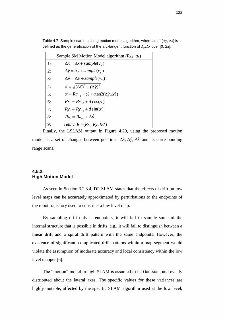
122
Table 4.7: Sample scan matching motion model algorithm, where atan2(Δy, Δx) is
defined as the generalization of the arc-tangent function of Δy/Δx over [0, 2π].
Sample SM Motion Model algorithm (Rt-1, ut )
1: )(ˆxvsamplexx
2: )(ˆyvsampleyy
3: )(ˆ vsample
4: 22 )ˆ()ˆ( yxd
5: )ˆ,ˆ(atan221 xyR t
6: )cos(1 dRxRx tt
7: )sin(1 dRyRy tt
8: ˆ1 tt RR
9: return Rt=(Rxt, Ryt,Rθt)
Finally, the LSLAM output in Figure 4.20, using the proposed motion
model, is a set of changes between positions zyx ˆ,ˆ,ˆ and its corresponding
range scans.
4.5.2. High Motion Model
As seen in Section 3.2.3.4, DP-SLAM states that the effects of drift on low
level maps can be accurately approximated by perturbations to the endpoints of
the robot trajectory used to construct a low level map.
By sampling drift only at endpoints, it will fail to sample some of the
internal structure that is possible in drifts, e.g., it will fail to distinguish between a
linear drift and a spiral drift pattern with the same endpoints. However, the
existence of significant, complicated drift patterns within a map segment would
violate the assumption of moderate accuracy and local consistency within the low
level mapper [6].
The “motion” model in high SLAM is assumed to be Gaussian, and evenly
distributed about the lateral axes. The specific values for these variances are
highly mutable, affected by the specific SLAM algorithm used at the low level,
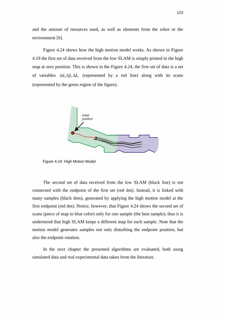
123
and the amount of resources used, as well as elements from the robot or the
environment [6].
Figure 4.24 shows how the high motion model works. As shown in Figure
4.19 the first set of data received from the low SLAM is simply printed in the high
map at zero position. This is shown in the Figure 4.24, the first set of data is a set
of variables ,ˆ,ˆ,ˆ zyx (represented by a red line) along with its scans
(represented by the green region of the figure).
Figure 4.24: High Motion Model
The second set of data received from the low SLAM (black line) is not
connected with the endpoint of the first set (red dot). Instead, it is linked with
many samples (black dots), generated by applying the high motion model at the
first endpoint (red dot). Notice, however, that Figure 4.24 shows the second set of
scans (piece of map in blue color) only for one sample (the best sample); thus it is
understood that high SLAM keeps a different map for each sample. Note that the
motion model generates samples not only disturbing the endpoint position, but
also the endpoint rotation.
In the next chapter the presented algorithms are evaluated, both using
simulated data and real experimental data taken from the literature.

124
125
5. Tests and results
This chapter presents results obtained using the proposed method on
simulated and real data. First, it is analyzed the scan matching optimization; after
that, the Scan Matching Motion Model is detailed presented, then some 2D results
are shown using DP-SLAM; and finally a simulated and a real 3D map example
are presented.
5.1. Scan Matching
5.1.1. Optimization Parameters Influence
Because this analysis uses simulated data, the truth robot displacement
values, Δx, Δy, Δθ; are known exactly; this will help us to test the optimization
parameters influence on the scan matching process.
As shown in Section 4.4.2, the optimization using genetic algorithm
depends on the size of the population and the number of generations. The Figure
5.1 and Figure 5.2 present the error displacement obtained by scan matching,
showing the population size influence in DE optimization (the number of
generation is kept fixed, in this case generations = 50), this experiment has 366
simulated robot poses and were acquired by simulating an standard deviation error
of 15 mm.
Notice that in Figure 5.1, small population leads to non-convergence and
consequently the estimated displacement surfers from hug errors, as shown in this
case for population size of 20 and 40.
In the other hand Figure 5.2, shows the same experiment using a larger
population; here the peaks have been significantly reduced in size and number
(see the scale).
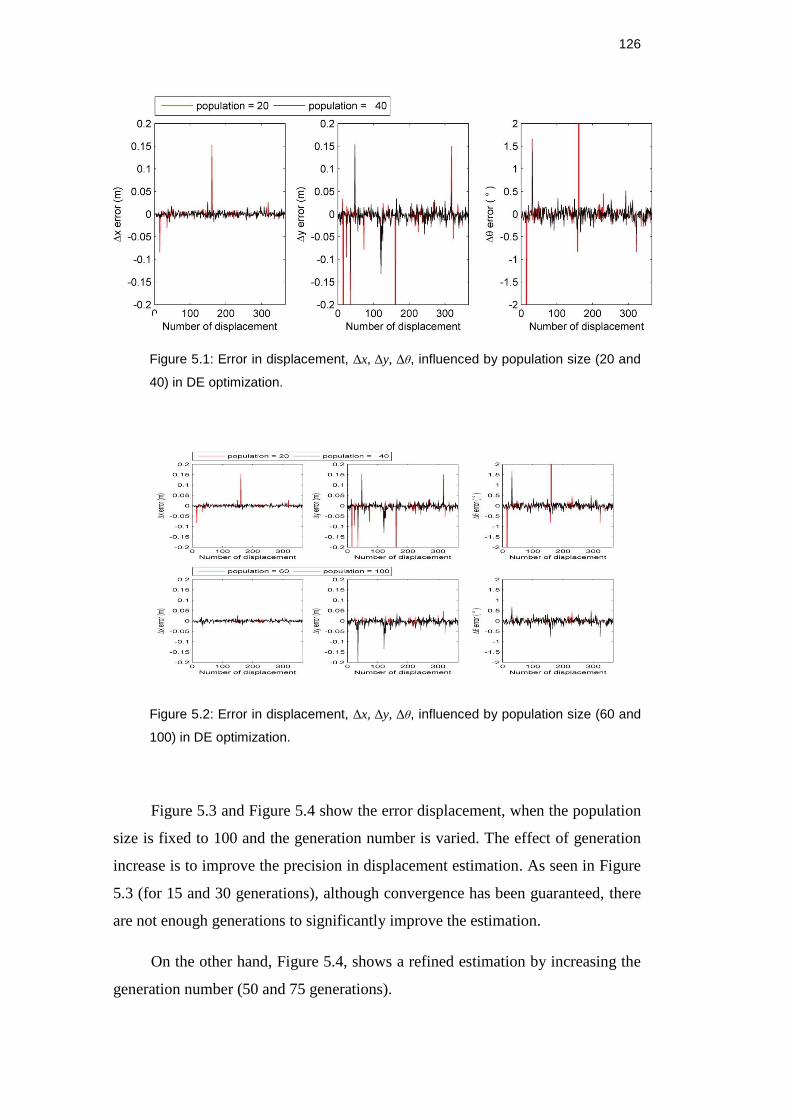
126
Figure 5.1: Error in displacement, Δx, Δy, Δθ, influenced by population size (20 and
40) in DE optimization.
Figure 5.2: Error in displacement, Δx, Δy, Δθ, influenced by population size (60 and
100) in DE optimization.
Figure 5.3 and Figure 5.4 show the error displacement, when the population
size is fixed to 100 and the generation number is varied. The effect of generation
increase is to improve the precision in displacement estimation. As seen in Figure
5.3 (for 15 and 30 generations), although convergence has been guaranteed, there
are not enough generations to significantly improve the estimation.
On the other hand, Figure 5.4, shows a refined estimation by increasing the
generation number (50 and 75 generations).
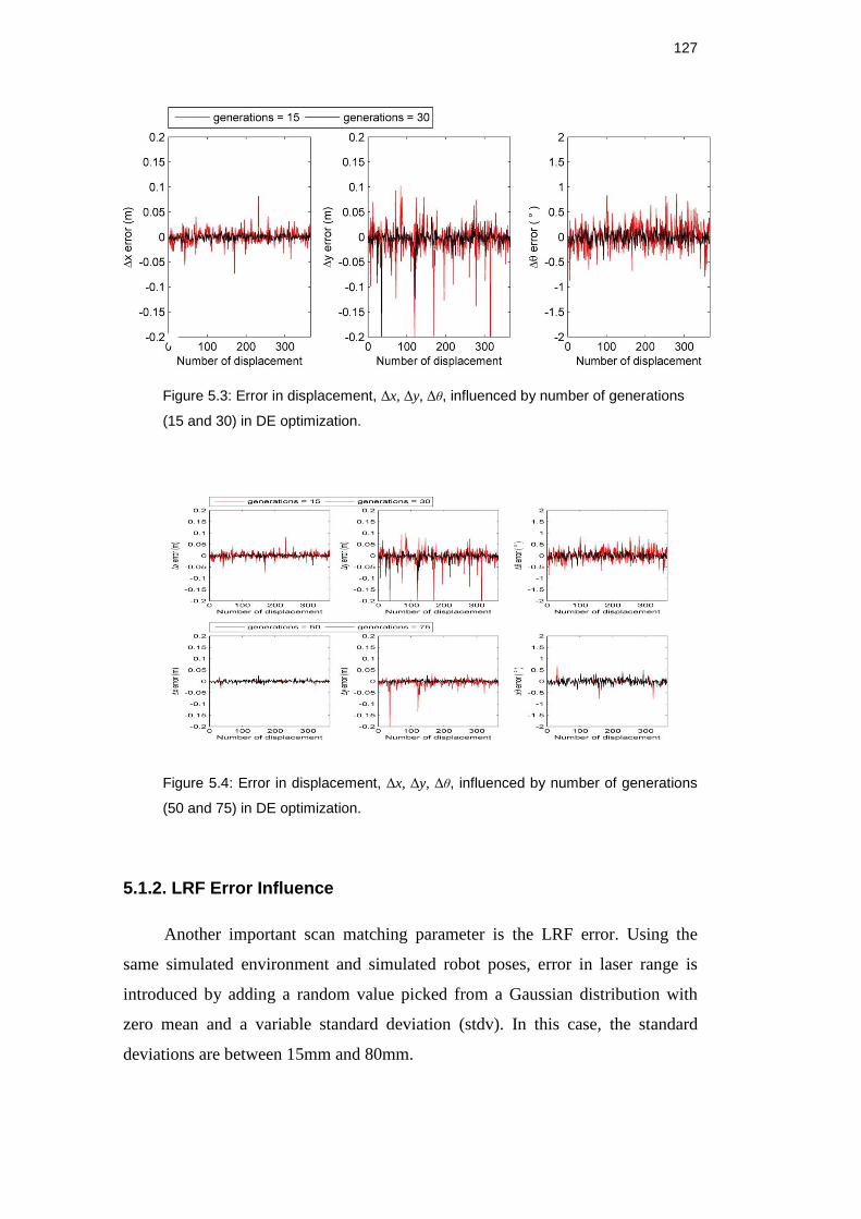
127
Figure 5.3: Error in displacement, Δx, Δy, Δθ, influenced by number of generations
(15 and 30) in DE optimization.
Figure 5.4: Error in displacement, Δx, Δy, Δθ, influenced by number of generations
(50 and 75) in DE optimization.
5.1.2. LRF Error Influence
Another important scan matching parameter is the LRF error. Using the
same simulated environment and simulated robot poses, error in laser range is
introduced by adding a random value picked from a Gaussian distribution with
zero mean and a variable standard deviation (stdv). In this case, the standard
deviations are between 15mm and 80mm.
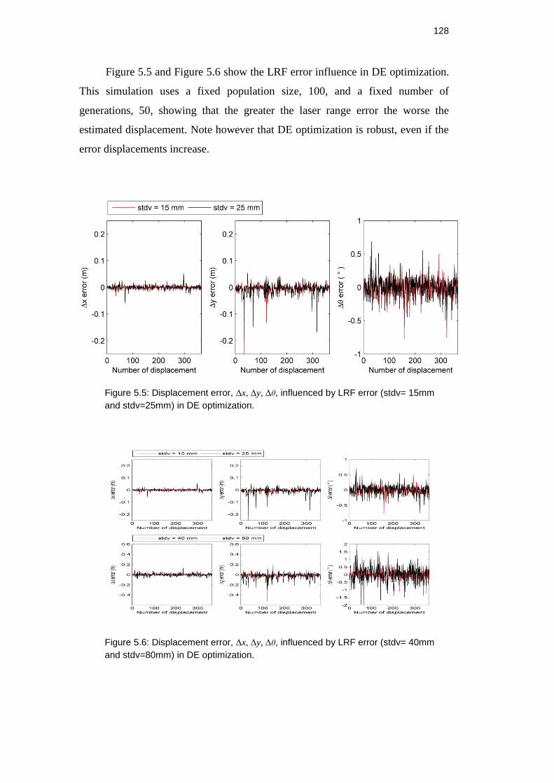
128
Figure 5.5 and Figure 5.6 show the LRF error influence in DE optimization.
This simulation uses a fixed population size, 100, and a fixed number of
generations, 50, showing that the greater the laser range error the worse the
estimated displacement. Note however that DE optimization is robust, even if the
error displacements increase.
Figure 5.5: Displacement error, Δx, Δy, Δθ, influenced by LRF error (stdv= 15mm
and stdv=25mm) in DE optimization.
Figure 5.6: Displacement error, Δx, Δy, Δθ, influenced by LRF error (stdv= 40mm
and stdv=80mm) in DE optimization.
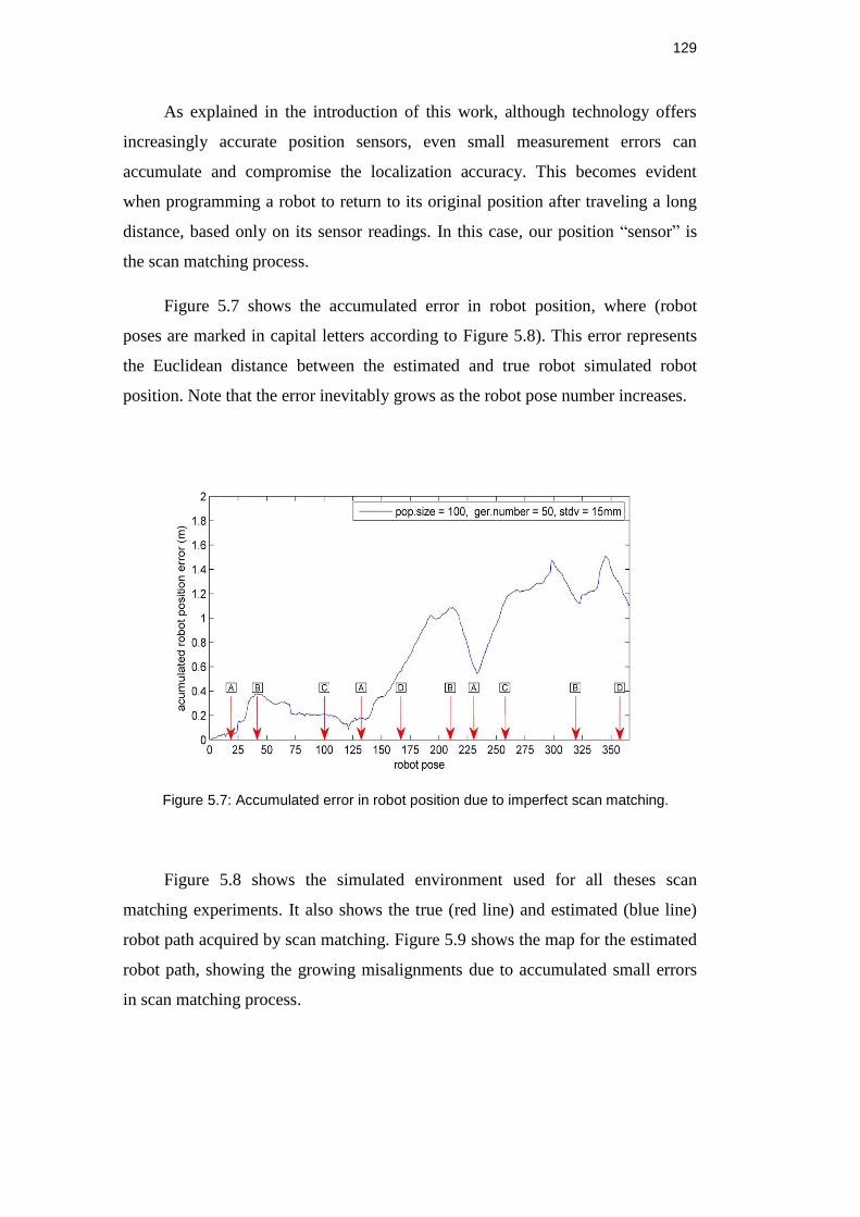
129
As explained in the introduction of this work, although technology offers
increasingly accurate position sensors, even small measurement errors can
accumulate and compromise the localization accuracy. This becomes evident
when programming a robot to return to its original position after traveling a long
distance, based only on its sensor readings. In this case, our position “sensor” is
the scan matching process.
Figure 5.7 shows the accumulated error in robot position, where (robot
poses are marked in capital letters according to Figure 5.8). This error represents
the Euclidean distance between the estimated and true robot simulated robot
position. Note that the error inevitably grows as the robot pose number increases.
Figure 5.7: Accumulated error in robot position due to imperfect scan matching.
Figure 5.8 shows the simulated environment used for all theses scan
matching experiments. It also shows the true (red line) and estimated (blue line)
robot path acquired by scan matching. Figure 5.9 shows the map for the estimated
robot path, showing the growing misalignments due to accumulated small errors
in scan matching process.
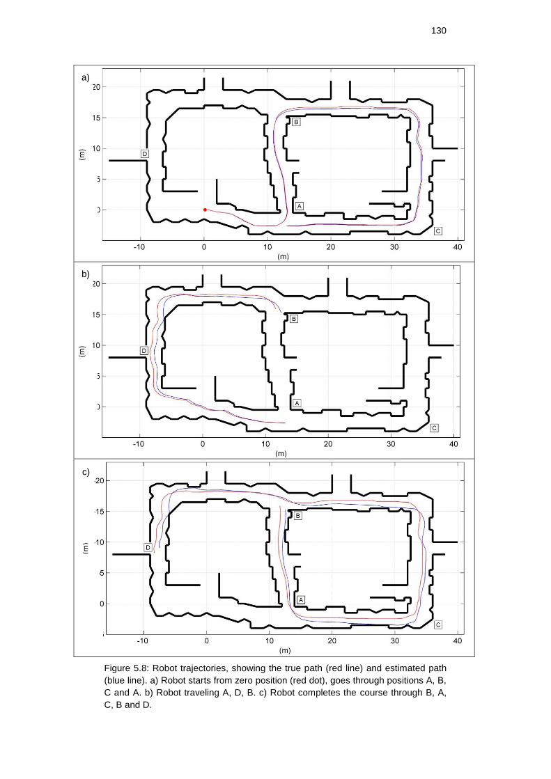
130
Figure 5.8: Robot trajectories, showing the true path (red line) and estimated path
(blue line). a) Robot starts from zero position (red dot), goes through positions A, B,
C and A. b) Robot traveling A, D, B. c) Robot completes the course through B, A,
C, B and D.
a
d
s
a)
b)
c)
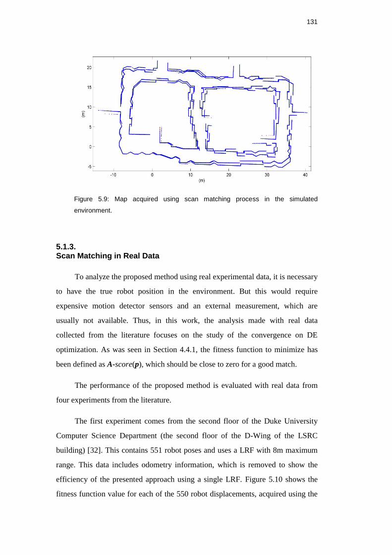
131
Figure 5.9: Map acquired using scan matching process in the simulated
environment.
5.1.3. Scan Matching in Real Data
To analyze the proposed method using real experimental data, it is necessary
to have the true robot position in the environment. But this would require
expensive motion detector sensors and an external measurement, which are
usually not available. Thus, in this work, the analysis made with real data
collected from the literature focuses on the study of the convergence on DE
optimization. As was seen in Section 4.4.1, the fitness function to minimize has
been defined as A-score(p), which should be close to zero for a good match.
The performance of the proposed method is evaluated with real data from
four experiments from the literature.
The first experiment comes from the second floor of the Duke University
Computer Science Department (the second floor of the D-Wing of the LSRC
building) [32]. This contains 551 robot poses and uses a LRF with 8m maximum
range. This data includes odometry information, which is removed to show the
efficiency of the presented approach using a single LRF. Figure 5.10 shows the
fitness function value for each of the 550 robot displacements, acquired using the
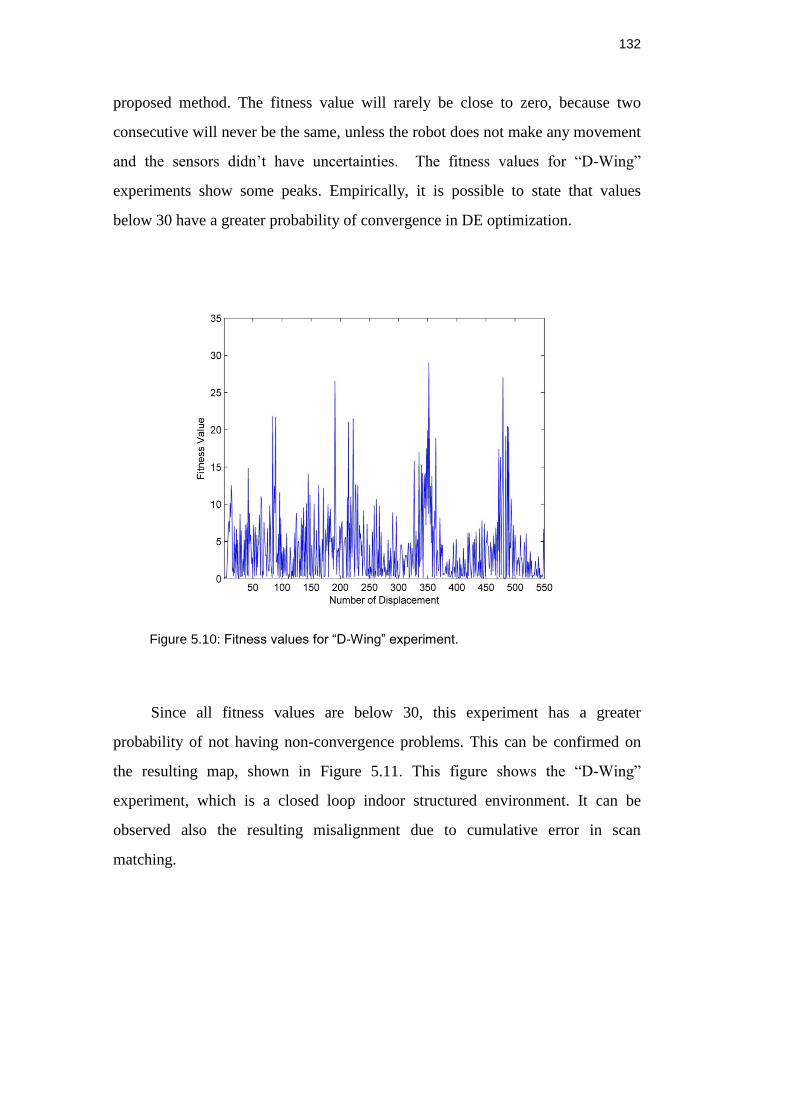
132
proposed method. The fitness value will rarely be close to zero, because two
consecutive will never be the same, unless the robot does not make any movement
and the sensors didn’t have uncertainties. The fitness values for “D-Wing”
experiments show some peaks. Empirically, it is possible to state that values
below 30 have a greater probability of convergence in DE optimization.
Figure 5.10: Fitness values for “D-Wing” experiment.
Since all fitness values are below 30, this experiment has a greater
probability of not having non-convergence problems. This can be confirmed on
the resulting map, shown in Figure 5.11. This figure shows the “D-Wing”
experiment, which is a closed loop indoor structured environment. It can be
observed also the resulting misalignment due to cumulative error in scan
matching.
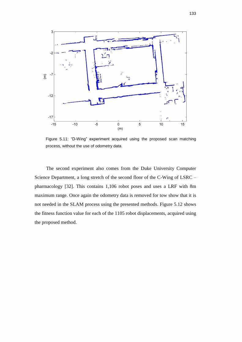
133
Figure 5.11: “D-Wing” experiment acquired using the proposed scan matching
process, without the use of odometry data.
The second experiment also comes from the Duke University Computer
Science Department, a long stretch of the second floor of the C-Wing of LSRC –
pharmacology [32]. This contains 1,106 robot poses and uses a LRF with 8m
maximum range. Once again the odometry data is removed for tow show that it is
not needed in the SLAM process using the presented methods. Figure 5.12 shows
the fitness function value for each of the 1105 robot displacements, acquired using
the proposed method.
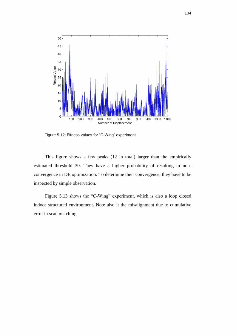
134
Figure 5.12: Fitness values for “C-Wing” experiment
This figure shows a few peaks (12 in total) larger than the empirically
estimated threshold 30. They have a higher probability of resulting in non-
convergence in DE optimization. To determine their convergence, they have to be
inspected by simple observation.
Figure 5.13 shows the “C-Wing” experiment, which is also a loop closed
indoor structured environment. Note also it the misalignment due to cumulative
error in scan matching.
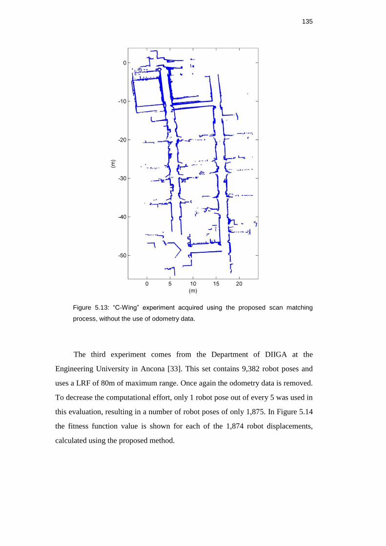
135
Figure 5.13: “C-Wing” experiment acquired using the proposed scan matching
process, without the use of odometry data.
The third experiment comes from the Department of DIIGA at the
Engineering University in Ancona [33]. This set contains 9,382 robot poses and
uses a LRF of 80m of maximum range. Once again the odometry data is removed.
To decrease the computational effort, only 1 robot pose out of every 5 was used in
this evaluation, resulting in a number of robot poses of only 1,875. In Figure 5.14
the fitness function value is shown for each of the 1,874 robot displacements,
calculated using the proposed method.
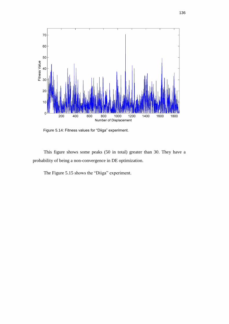
136
Figure 5.14: Fitness values for “Diiga” experiment.
This figure shows some peaks (50 in total) greater than 30. They have a
probability of being a non-convergence in DE optimization.
The Figure 5.15 shows the “Diiga” experiment.
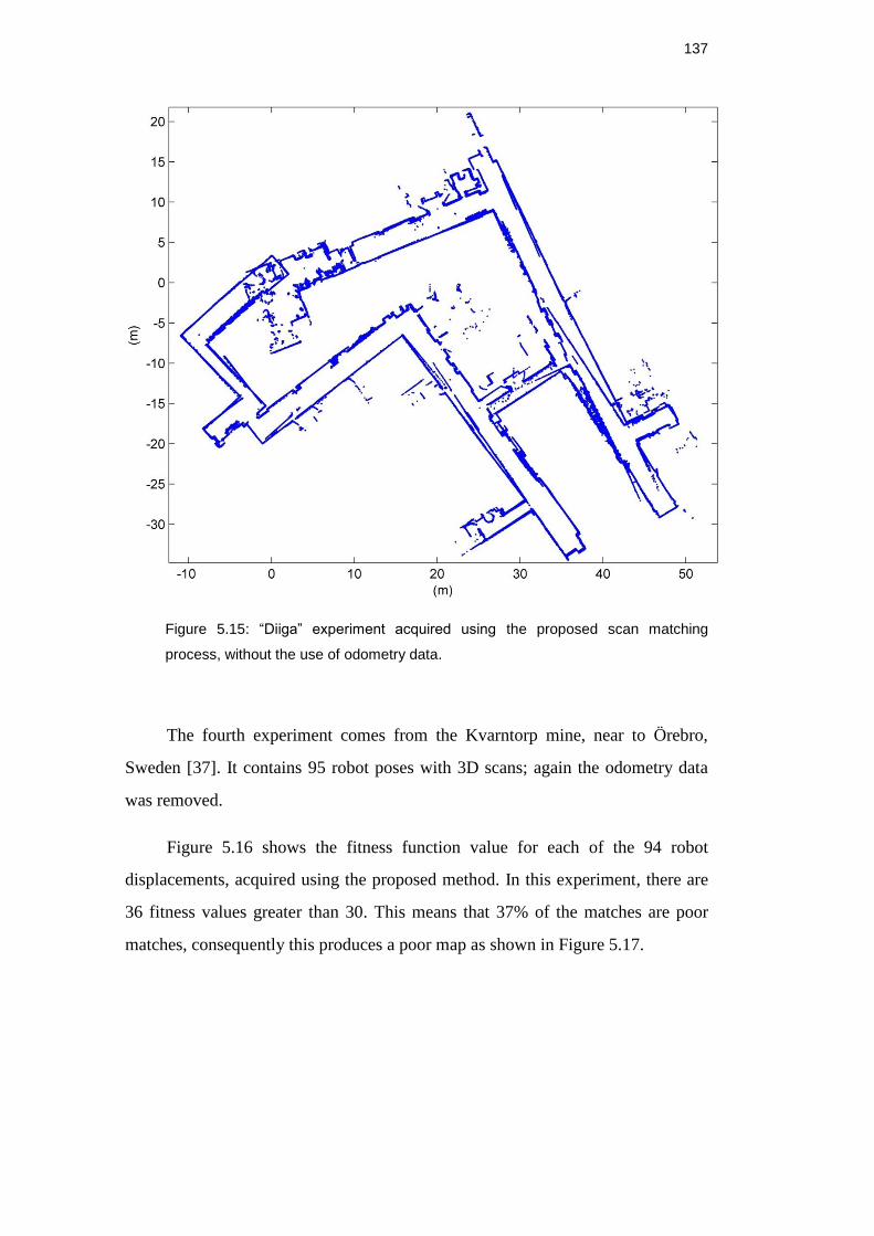
137
Figure 5.15: “Diiga” experiment acquired using the proposed scan matching
process, without the use of odometry data.
The fourth experiment comes from the Kvarntorp mine, near to Örebro,
Sweden [37]. It contains 95 robot poses with 3D scans; again the odometry data
was removed.
Figure 5.16 shows the fitness function value for each of the 94 robot
displacements, acquired using the proposed method. In this experiment, there are
36 fitness values greater than 30. This means that 37% of the matches are poor
matches, consequently this produces a poor map as shown in Figure 5.17.
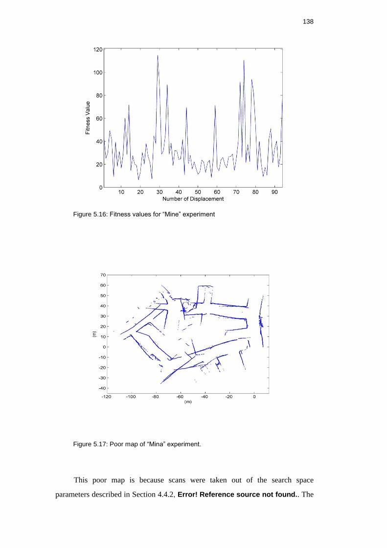
138
Figure 5.16: Fitness values for “Mine” experiment
Figure 5.17: Poor map of “Mina” experiment.
This poor map is because scans were taken out of the search space
parameters described in Section 4.4.2, Error! Reference source not found.. The
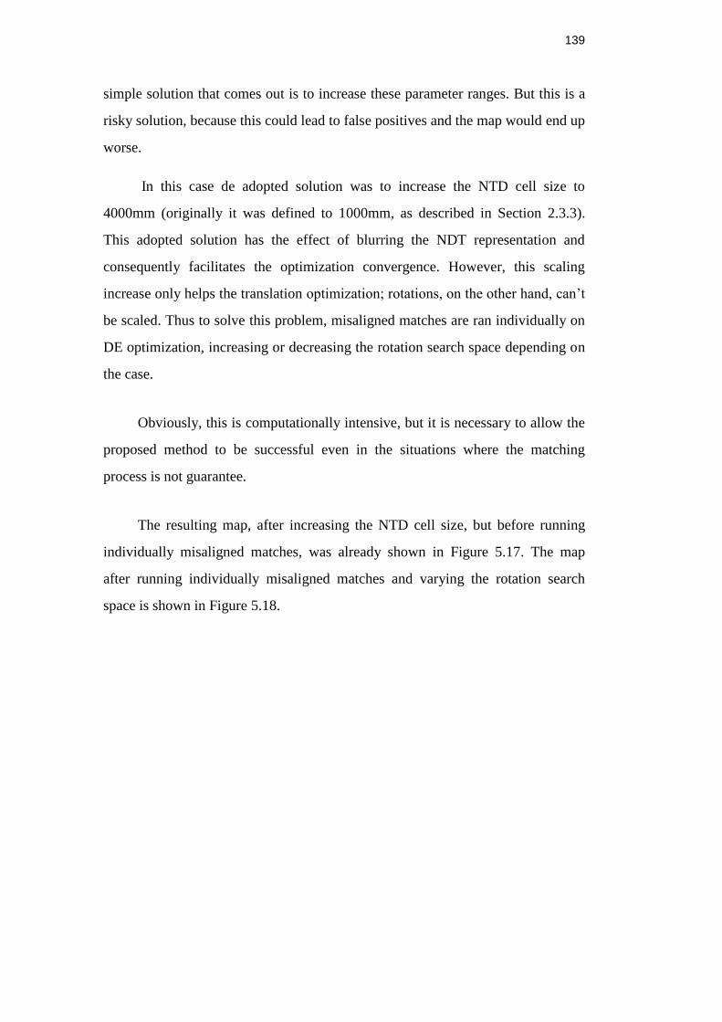
139
simple solution that comes out is to increase these parameter ranges. But this is a
risky solution, because this could lead to false positives and the map would end up
worse.
In this case de adopted solution was to increase the NTD cell size to
4000mm (originally it was defined to 1000mm, as described in Section 2.3.3).
This adopted solution has the effect of blurring the NDT representation and
consequently facilitates the optimization convergence. However, this scaling
increase only helps the translation optimization; rotations, on the other hand, can’t
be scaled. Thus to solve this problem, misaligned matches are ran individually on
DE optimization, increasing or decreasing the rotation search space depending on
the case.
Obviously, this is computationally intensive, but it is necessary to allow the
proposed method to be successful even in the situations where the matching
process is not guarantee.
The resulting map, after increasing the NTD cell size, but before running
individually misaligned matches, was already shown in Figure 5.17. The map
after running individually misaligned matches and varying the rotation search
space is shown in Figure 5.18.
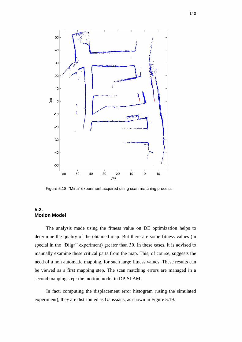
140
Figure 5.18: “Mina” experiment acquired using scan matching process
5.2. Motion Model
The analysis made using the fitness value on DE optimization helps to
determine the quality of the obtained map. But there are some fitness values (in
special in the “Diiga” experiment) greater than 30. In these cases, it is advised to
manually examine these critical parts from the map. This, of course, suggests the
need of a non automatic mapping, for such large fitness values. These results can
be viewed as a first mapping step. The scan matching errors are managed in a
second mapping step: the motion model in DP-SLAM.
In fact, computing the displacement error histogram (using the simulated
experiment), they are distributed as Gaussians, as shown in Figure 5.19.
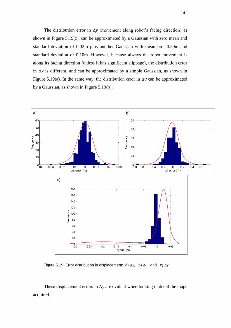
141
The distribution error in Δy (movement along robot’s facing direction) as
shown in Figure 5.19(c), can be approximated by a Gaussian with zero mean and
standard deviation of 0.02m plus another Gaussian with mean on 0.20m and
standard deviation of 0.10m. However, because always the robot movement is
along its facing direction (unless it has significant slippage), the distribution error
in Δx is different, and can be approximated by a simple Gaussian, as shown in
Figure 5.19(a). In the same way, the distribution error in Δθ can be approximated
by a Gaussian, as shown in Figure 5.19(b).
a)
b)
c)
Figure 5.19: Error distribution in displacement: a) Δx, b) Δθ and c) Δy
These displacement errors in Δy are evident when looking in detail the maps
acquired.
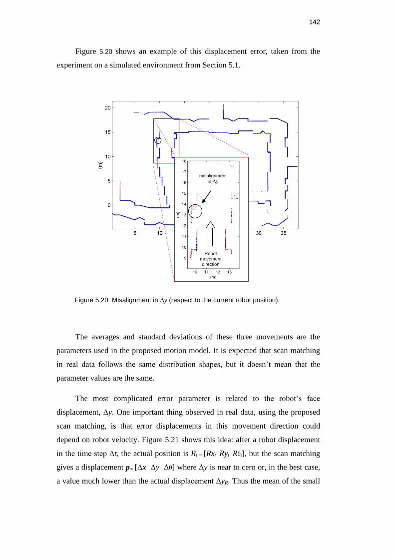
142
Figure 5.20 shows an example of this displacement error, taken from the
experiment on a simulated environment from Section 5.1.
Figure 5.20: Misalignment in Δy (respect to the current robot position).
The averages and standard deviations of these three movements are the
parameters used in the proposed motion model. It is expected that scan matching
in real data follows the same distribution shapes, but it doesn’t mean that the
parameter values are the same.
The most complicated error parameter is related to the robot’s face
displacement, Δy. One important thing observed in real data, using the proposed
scan matching, is that error displacements in this movement direction could
depend on robot velocity. Figure 5.21 shows this idea: after a robot displacement
in the time step Δt, the actual position is Rt = [Rxt Ryt Rθt], but the scan matching
gives a displacement p= [Δx Δy Δθ] where Δy is near to cero or, in the best case,
a value much lower than the actual displacement ΔyR. Thus the mean of the small
misalignment
in Δy
Robot movement direction
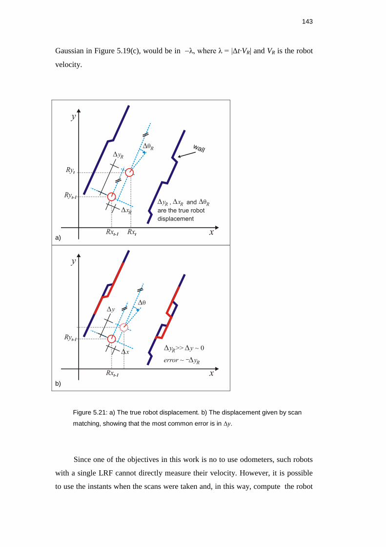
143
Gaussian in Figure 5.19(c), would be in λ, where λ = |Δt·VR| and VR is the robot
velocity.
a)
b)
Figure 5.21: a) The true robot displacement. b) The displacement given by scan
matching, showing that the most common error is in Δy.
Since one of the objectives in this work is no to use odometers, such robots
with a single LRF cannot directly measure their velocity. However, it is possible
to use the instants when the scans were taken and, in this way, compute the robot
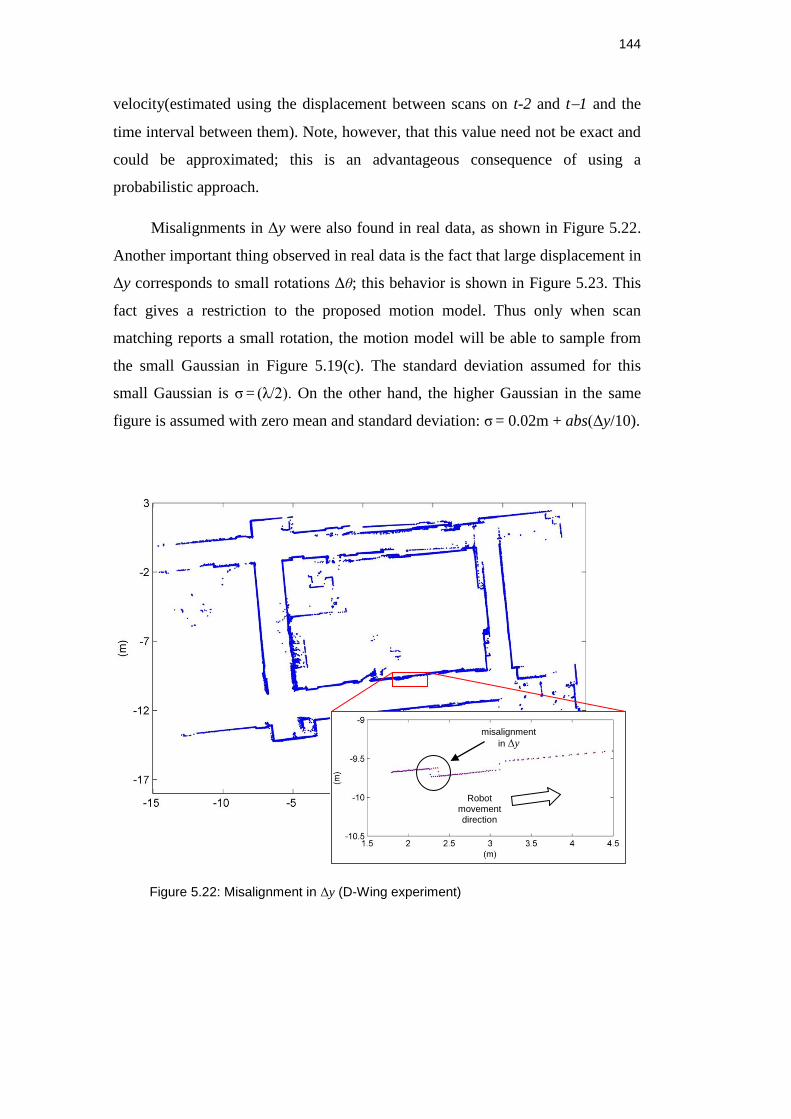
144
velocity(estimated using the displacement between scans on t-2 and t1 and the
time interval between them). Note, however, that this value need not be exact and
could be approximated; this is an advantageous consequence of using a
probabilistic approach.
Misalignments in Δy were also found in real data, as shown in Figure 5.22.
Another important thing observed in real data is the fact that large displacement in
Δy corresponds to small rotations Δθ; this behavior is shown in Figure 5.23. This
fact gives a restriction to the proposed motion model. Thus only when scan
matching reports a small rotation, the motion model will be able to sample from
the small Gaussian in Figure 5.19(c). The standard deviation assumed for this
small Gaussian is σ = (λ/2). On the other hand, the higher Gaussian in the same
figure is assumed with zero mean and standard deviation: σ = 0.02m + abs(Δy/10).
Figure 5.22: Misalignment in Δy (D-Wing experiment)
Robot movement direction
misalignment
in Δy
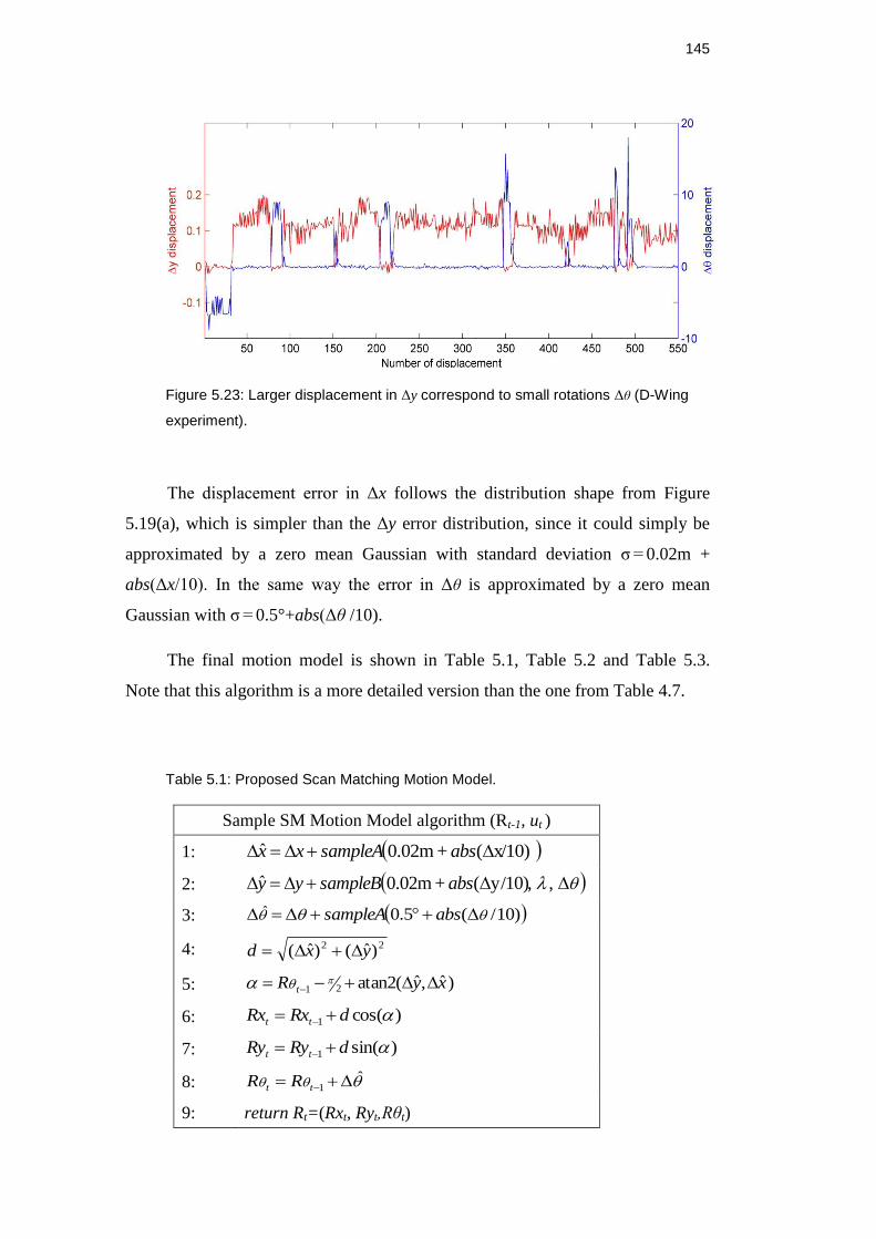
145
Figure 5.23: Larger displacement in Δy correspond to small rotations Δθ (D-Wing
experiment).
The displacement error in Δx follows the distribution shape from Figure
5.19(a), which is simpler than the Δy error distribution, since it could simply be
approximated by a zero mean Gaussian with standard deviation σ = 0.02m +
abs(Δx/10). In the same way the error in Δθ is approximated by a zero mean
Gaussian with σ = 0.5°+abs(Δθ /10).
The final motion model is shown in Table 5.1, Table 5.2 and Table 5.3.
Note that this algorithm is a more detailed version than the one from Table 4.7.
Table 5.1: Proposed Scan Matching Motion Model.
Sample SM Motion Model algorithm (Rt-1, ut )
1: x/10)( + 0.02mˆ abssampleAxx
2: ,,y/10)( + 0.02mˆ abssampleByy
3: )10/(5.0ˆ abssampleA
4: 22 )ˆ()ˆ( yxd
5: )ˆ,ˆ(atan221 xyR t
6: )cos(1 dRxRx tt
7: )sin(1 dRyRy tt
8: ˆ1 tt RR
9: return Rt=(Rxt, Ryt,Rθt)
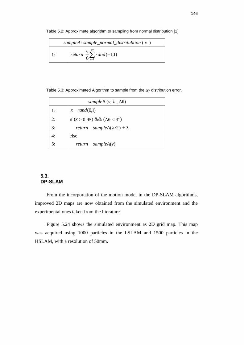
146
Table 5.2: Approximate algorithm to sampling from normal distribution [1]
sampleA: sample_normal_distritubtion ( v )
1:
12
1
)1,1(6 i
randv
return
Table 5.3: Approximated Algorithm to sample from the Δy distribution error.
sampleB (v, λ , Δθ)
1: )1,0(randx
2: if (x > 0.95) && (Δθ < 3°)
3: return sampleA(λ/2) + λ
4: else
5: return sampleA(v)
5.3. DP-SLAM
From the incorporation of the motion model in the DP-SLAM algorithms,
improved 2D maps are now obtained from the simulated environment and the
experimental ones taken from the literature.
Figure 5.24 shows the simulated environment as 2D grid map. This map
was acquired using 1000 particles in the LSLAM and 1500 particles in the
HSLAM, with a resolution of 50mm.
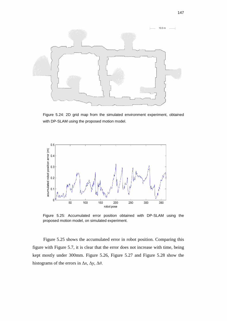
147
Figure 5.24: 2D grid map from the simulated environment experiment, obtained
with DP-SLAM using the proposed motion model.
Figure 5.25: Accumulated error position obtained with DP-SLAM using the
proposed motion model, on simulated experiment.
Figure 5.25 shows the accumulated error in robot position. Comparing this
figure with Figure 5.7, it is clear that the error does not increase with time, being
kept mostly under 300mm. Figure 5.26, Figure 5.27 and Figure 5.28 show the
histograms of the errors in Δx, Δy, Δθ.
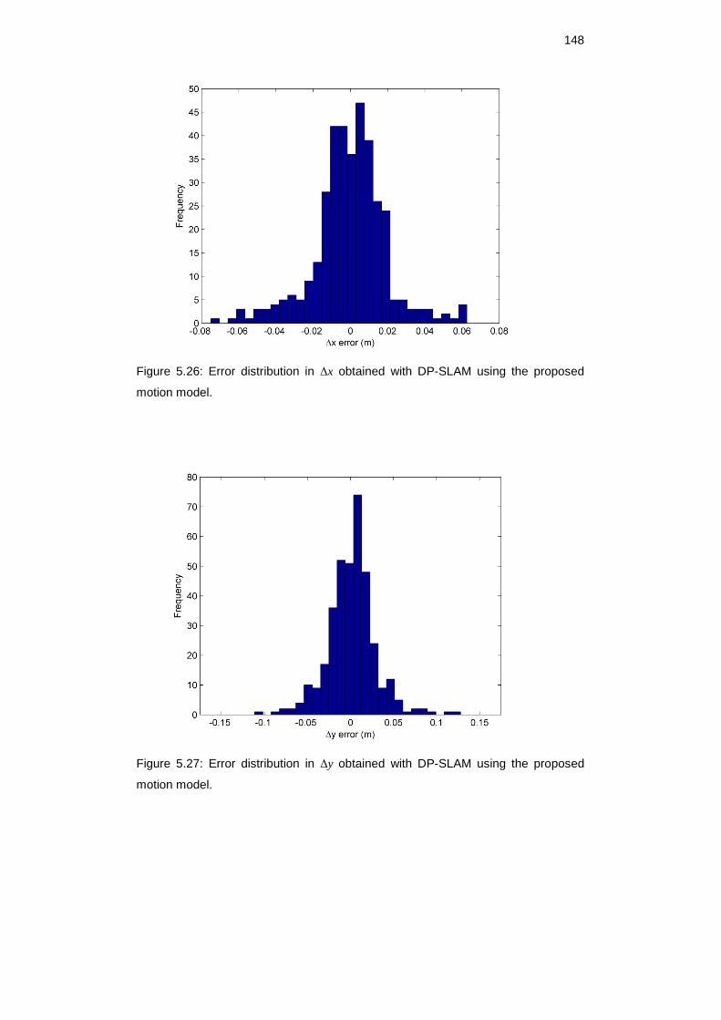
148
Figure 5.26: Error distribution in Δx obtained with DP-SLAM using the proposed
motion model.
Figure 5.27: Error distribution in Δy obtained with DP-SLAM using the proposed
motion model.
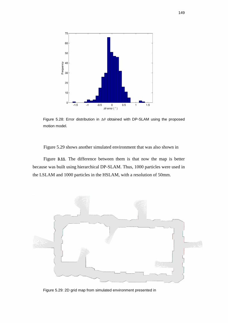
149
Figure 5.28: Error distribution in Δθ obtained with DP-SLAM using the proposed
motion model.
Figure 5.29 shows another simulated environment that was also shown in
Figure 3.11. The difference between them is that now the map is better
because was built using hierarchical DP-SLAM. Thus, 1000 particles were used in
the LSLAM and 1000 particles in the HSLAM, with a resolution of 50mm.
Figure 5.29: 2D grid map from simulated environment presented in
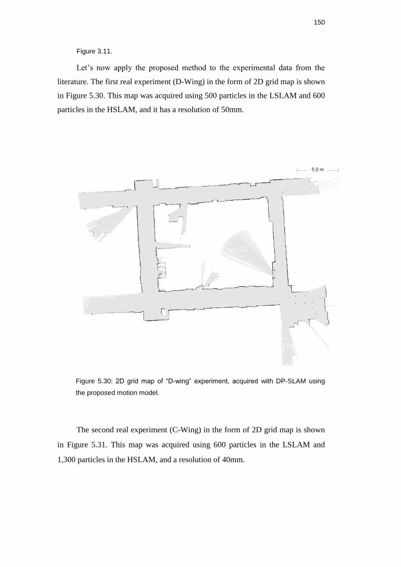
150
Figure 3.11.
Let’s now apply the proposed method to the experimental data from the
literature. The first real experiment (D-Wing) in the form of 2D grid map is shown
in Figure 5.30. This map was acquired using 500 particles in the LSLAM and 600
particles in the HSLAM, and it has a resolution of 50mm.
Figure 5.30: 2D grid map of “D-wing” experiment, acquired with DP-SLAM using
the proposed motion model.
The second real experiment (C-Wing) in the form of 2D grid map is shown
in Figure 5.31. This map was acquired using 600 particles in the LSLAM and
1,300 particles in the HSLAM, and a resolution of 40mm.
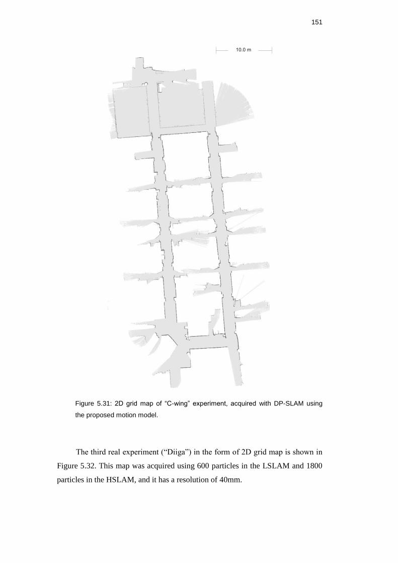
151
Figure 5.31: 2D grid map of “C-wing” experiment, acquired with DP-SLAM using
the proposed motion model.
The third real experiment (“Diiga”) in the form of 2D grid map is shown in
Figure 5.32. This map was acquired using 600 particles in the LSLAM and 1800
particles in the HSLAM, and it has a resolution of 40mm.
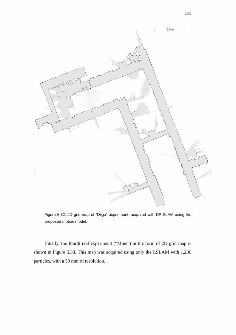
152
Figure 5.32: 2D grid map of “Diiga” experiment, acquired with DP-SLAM using the
proposed motion model.
Finally, the fourth real experiment (“Mine”) in the form of 2D grid map is
shown in Figure 5.33. This map was acquired using only the LSLAM with 1,200
particles, with a 50 mm of resolution.
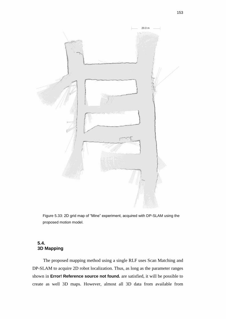
153
Figure 5.33: 2D grid map of “Mine” experiment, acquired with DP-SLAM using the
proposed motion model.
5.4. 3D Mapping
The proposed mapping method using a single RLF uses Scan Matching and
DP-SLAM to acquire 2D robot localization. Thus, as long as the parameter ranges
shown in Error! Reference source not found. are satisfied, it will be possible to
create as well 3D maps. However, almost all 3D data from available from
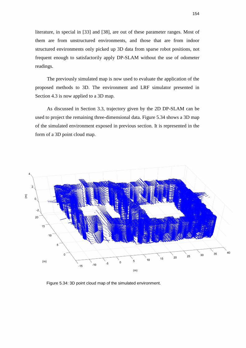
154
literature, in special in [33] and [38], are out of these parameter ranges. Most of
them are from unstructured environments, and those that are from indoor
structured environments only picked up 3D data from sparse robot positions, not
frequent enough to satisfactorily apply DP-SLAM without the use of odometer
readings.
The previously simulated map is now used to evaluate the application of the
proposed methods to 3D. The environment and LRF simulator presented in
Section 4.3 is now applied to a 3D map.
As discussed in Section 3.3, trajectory given by the 2D DP-SLAM can be
used to project the remaining three-dimensional data. Figure 5.34 shows a 3D map
of the simulated environment exposed in previous section. It is represented in the
form of a 3D point cloud map.
Figure 5.34: 3D point cloud map of the simulated environment.
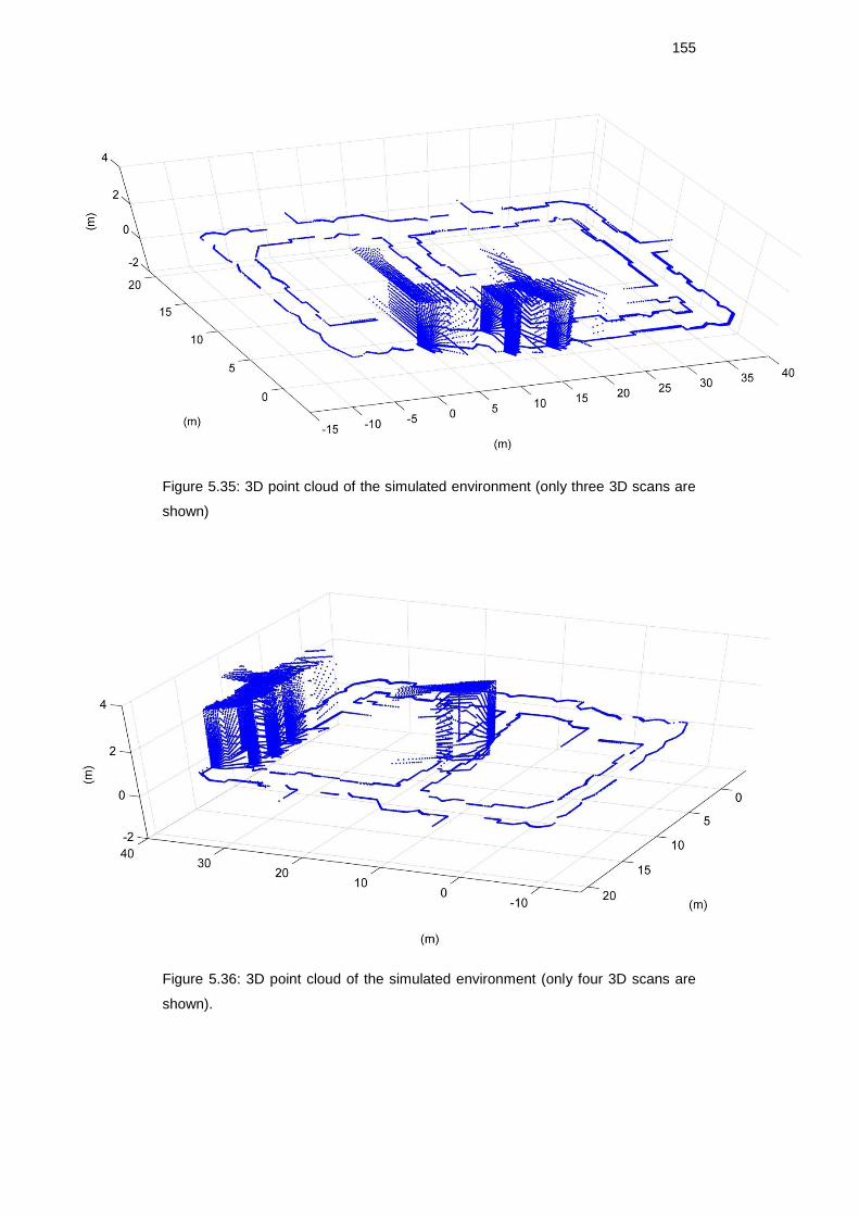
155
Figure 5.35: 3D point cloud of the simulated environment (only three 3D scans are
shown)
Figure 5.36: 3D point cloud of the simulated environment (only four 3D scans are
shown).
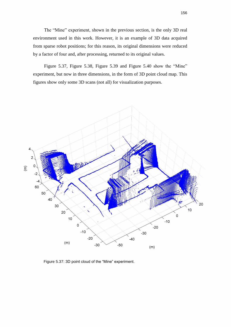
156
The “Mine” experiment, shown in the previous section, is the only 3D real
environment used in this work. However, it is an example of 3D data acquired
from sparse robot positions; for this reason, its original dimensions were reduced
by a factor of four and, after processing, returned to its original values.
Figure 5.37, Figure 5.38, Figure 5.39 and Figure 5.40 show the “Mine”
experiment, but now in three dimensions, in the form of 3D point cloud map. This
figures show only some 3D scans (not all) for visualization purposes.
Figure 5.37: 3D point cloud of the “Mine” experiment.
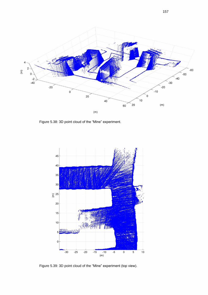
157
Figure 5.38: 3D point cloud of the “Mine” experiment.
Figure 5.39: 3D point cloud of the “Mine” experiment (top view).
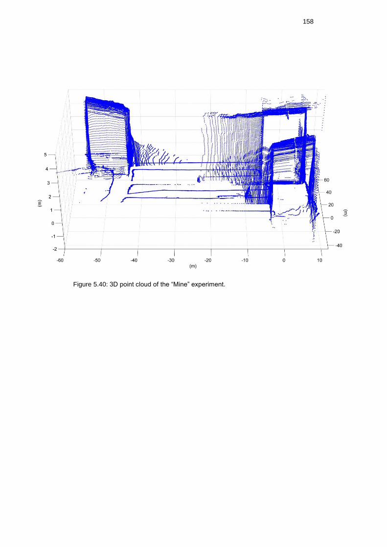
158
Figure 5.40: 3D point cloud of the “Mine” experiment.

159
6. Conclusions
This work explored the main SLAM solutions, given a detailed example for
implementing the EKF-SLAM and FastSLAM; although the adopted solution, for
the proposed application, was the DP-SLAM.
Thus, to perform SLAM without odometry information, the following
algorithms were implemented:
A simulator to acquire 3D data from structured environments; implemented
on MatLab® platform.
A scan matching algorithm, to get robot displacement without odometry
information, based in genetic algorithm optimization for the Normal
Distribution Transform; also implemented on MatLab® platform, using the
Differential Evolution library acquired from reference [21].
A modified DP-SLAM, which included a new motion model: the scan
matching motion model; implemented on Visual C++ platform.
This method can deal as well with 3D environments, as long as the LRF is
mounted on a rotating platform on the mobile robot, to allow both horizontal and
vertical scans. As the robot moves, the LRF acquires 2D scans. Where and when
3D data is required, the robot stops and the platform rotates synchronized with the
LRF to perform further 2D scans on different plane orientations. After traveling
through a desired path, the acquired data is processed to obtain 2D or 3D maps.
In this way, the main contribution of this thesis is the application of DP-
SLAM without the need for odometry information, just by using a single LRF.
Furthermore, this comes with some considerations and advices, along with
specific conclusions, detailed next.
160
6.1. DP-SLAM Conclusions
DP-SLAM is a powerful tool in 2D mapping so that, it doesn’t need a
separated loop detection algorithm.
Such a high performance comes with a high computational cost. Thus, DP-
SLAM is an off-line mapping algorithm, due to the huge data it manages. The
smallest experiment (“Mine”) took about 1 hour to be evaluated and the longest
(“Diiga”) took about 5 hours, using a processor AMD Turion 64 with 2.1GHz.
The time complexity of DP-SLAM is analyzed in detail in [6].
The Motion Model in DP-SLAM has a considerable influence in the
mapping performance. Poor models will need a huge number of particles to obtain
moderate results. Thus, the Scan Matching Motion Model proposed in this work
could be improved to include holonomic robots, so that they can manage both Δx
displacement errors as well as in Δy errors.
The “low map” size in LSLAM (“piece of data” in Figure 4.19) as proposed
by [6] is a function of the number of iterations. Thus, [6] proposes between 75 to
150 iterations. But in the analysis in this thesis, these values didn’t give good
results. Basically, 150 iterations don’t guarantee that the robot travels enough
distance to be considered a low map. The robot could get hundreds of scans
without leaving the same room. In all experiments made by DP-SLAM in this
work, a low map is only created when robot travels about 3m in an approximately
straight path. It was observed that, when a low map is created (the LSLAM
algorithm finishes) within a fast robot rotation, the next low map (that uses a
portion of the previous map) suffers major ambiguities and tends to produces poor
particles.
In LSLAM, DP-SLAM uses the current map for particle weighing. The best
particle is used to grow the map, adding the new observation. If the robot
displacement is higher than the LRF’s maximum range, then DP-SLAM does not
have enough pieces of the map for particle weighing. Thus, it is recommended to
have a LRF with maximum range large enough to avoid this undesired situation.
161
As a way of demonstrating the proposed method performance, the simulated
map (Figure 5.8) is compared with the acquired map using DP-SLAM (Figure
5.24). Thus, in order to compare them, the contours (walls) of both maps are
selected and then converted to bitmaps. In this case the pixel to pixel comparison
gives 93.34% of similarity, this mean 6.66% of wrong pixels.
6.2. Scan Matching Conclusions
The time of convergence in DE optimization depends on population size and
generation number. Population size of 100 with 50 generations takes
approximately 18s using a processor AMD Turion 64 with 2.1GHz. This
relatively long time, coupled with time consumed by DP-SLAM algorithm, make
the proposed method an offline but robust solution.
Errors in Scan Matching, the first or any other, are outweighed by the
motion model proposed in Section 5.2. Note also that the first scan or any other
have the same level of reliability; thus, if the first scan, and consequently the first
grid map, is not good, it can be improved by the subsequent iterations (subsequent
scans), in the sense of a probabilistic fusion.
Misalignments found in scan matching (for Δy displacement) are due to the
cell size defined in Section 2.3.3. I.e. small details in the environment are blurred
in NDT representation, which leads to unclear limits in alignment. One solution
would be to reduce the cell size, but this creates an NDT representation with sharp
shape; this case, DE optimization would need a quite larger population to achieve
convergence. However, with some considerations, the cell size could be
dynamically defined, depending on the measured LRF values. Thus, if LRF
returns small distances, for instance less than 3m, then the cell size would be
reduced to 500 mm. For higher distances, 1m of cell size would be a good choice.
This idea was not implemented in this thesis, but it suggests future works to
determine the distance threshold for each cell size choice.
162
The LRF’s maximum range, as in DP-SLAM, is a very important parameter
in scan matching. Larger maxima mean more data (about the environment) in one
scan, which helps to improve the alignment.
The scan matching proposed was implemented in Matlab®, while DP-
SLAM was implemented in C++ (using the code from [32]). It is possible, of
course, to use the same computer language for Scan Matching and DP-SLAM. To
increase the algorithm speed, it is recommended to implement the scan matching
in C++ as well. A powerful library for evolutionary computing, GCOM [38], can
help in such task. This is a suggestion for future works.
There are solutions for 3D scan matching in non-planar terrain [39], [40]
and [41]. Thus, they could be used as a basis to extend the proposed method to a
3D mapping in uneven terrain, using as well a single LRF without odometry
information.
6.3. 3D Mapping Conclusions
The 3D maps presented in Section 5.4 use point cloud representation. Thus,
the quality of these maps depends on LRF error, because they are simply plotted
using the 2D trajectory given by DP-SLAM. However, DP-SLAM fuses
probabilistic observations made for each cell, so, as the cell is more often
observed as occupied, the darker it becomes. This idea could be applied in 3D
representations as well. Thus, 3D observation may also be fused, similarly to what
is done in 2D. Note that this does not mean using a 3D cell for localization or
perception model: this means only using the 3D cells to print a 3D map output by
fusing the available observations made at each 3D cell. This idea, however, was
not implemented in this thesis but it is another suggestion for future works.
Another representation for 3D maps could be in the form of geometric
planes. The Delaunay triangulation is a popular algorithm to create a simplified
representation of the environment in the form of triangles acquired from a point
cloud. There are commercial and open source software [42] specialized in
processing this kind of data.

163
164
7. References
[1] THRUN, SEBASTIAN et al. Probabilistic Robotics. Cambridge,
Massachusetts - London, England: The MIT Press, 2006.
[2] KLAFTER, RICHARD DAVID, THOMAS A. CHMIELEWSKI, and MICHAEL
NEGIN. Robotic Engineering: An Integrated Approach. Prentice, Hall, 1989.
[3] FERREIRA, EDSON DE PAULA. Robotica Básica. Rio de Janeiro, 1991.
[4] HIEBER-TREUER, BRADLEY. "An Introduction to Robot SLAM
(Simultaneous Localization And Mapping)." Edited by Bachelor of Arts in
Computer Science - Middlebury College. Middlebury, Vermount, USA, 2007.
[5] THRUN, SEBASTIAN. "Robotic Mapping: A Survey." Pittsburgh, PA 15213:
School of Computer Science - Carnegie Mellon University, February 2002.
[6] ELIAZAR, AUSTIN. "DP-SLAM." Department of Computer Science - Duke
University, 2005.
[7] MORAVEC, H. P., and A. ELFES. "High resolution maps from wide angle
sonar." St. Louis, Missouri: ICRA-85, 1985.
[8] BIBER, PETER. "The Normal Distributions Transform: A New Approach to
Laser Scan." Sand 14, 72070 Tüingen, Germany: University of Tübingen,
Germany, 2003.
[9] LU, FENG, and EVANGELOS MILIOS. "Robot Pose Estimation in Unknown
Environments by Matching 2D Range Scans." North York, Canada M3J 1P3:
Department of Computer Science, York University, 1994.
[10] ALSHAWA, M. "ICL: Iterative Closest Line a Novel Point Cloud Registration
Algorithm Based on Linear Features." STRASBOURG, France:
Photogrammetry and Geomatics Group MAP-PAGE UMR 694, 2007.
[11] AGHAMOHAMMADI, A. A., H. D. TAGHIRAD, A. H. TAMJIDI, and E.
MIHANKHAH. "Feature-Based Laser Scan Matching For Accurate and High
Speed Mobile Robot Localization." Advanced Robotics and Automated
Systems (ARAS). Department of Electrical Engineering, K. N. Toosi
University of Technology, 2007.
165
[12] LINGEMANN, KAI, HARTMUT SURMANN, ANDREAS NÜCHTER, and
JOACHIM HERTZBERG. "Indoor and Outdoor Localization for Fast Mobile
Robots." Sankt Augustin, Germany: Fraunhofer Institute for Autonomous
Intelligent Systems (AIS), 2005.
[13] OLSON, EDWIN B. "Real-Time Correlative Scan Matching." Ann Arbor, MI,
USA: Department of Electrical Engineering and Computer Science -
University of Michigan, 2009.
[14] HOLLAND, John H. Adaption in Natural and Artificial Systems. Cambridge,
Massachusetts: MIT Press, 1992.
[15] MAN, K. F., K. S. TANG, and S. KWONG. "Genetic Algorithms: Concepts
and Applications." IEEE Transactions on Industrial Electronics, October
1996.
[16] DAVIS, LAWRENCE. "Handbook of Genetic Algorithms." New York: Davis,
Lawrence, January 1991.
[17] FORREST, STEPHANIE. "Genetic Algorithms: Principles of Natural
Selection Applied to Computation." Science Vol. 261, August 1993.
[18] NELSON, ANDREW L., GREGORY J BARLOW, and LEFTERIS
DOITSIDIS. "Fitness functions in evolutionary robotics: A survey and
analysis." ELSEVIER - Robotics and Autonomous Systems, September
2008.
[19] BABUA, B.V., and S.A. MUNAWARB. "Differential evolution strategies for
optimal design of shell-and-tube heat exchangers." ELSEVIER - Chemical
Engineering Science, April 2007.
[20] STORN, RAINER, and KENNETH PRICE. "Differential Evolution - A simple
and efficient adaptive scheme for global optimization over continuous
spaces." Berkeley, CA, USA: International Computer Science Institute,
March 1995.
[21] STORN, RAINER, and KENNETH PRICE. Differential Evolution (DE).
Availabel on: <http://www.ICSI.Berkeley.edu/~storn/code.html>. Accessed
in: June 2010.
[22] WELCH, GREG, and GARY BISHOP. "An Introduction to the Kalman Filter."
Chapel Hill, NC, USA: University of North Carolina at Chapel Hill, July 2006.
[23] MONTEMERLO, MICHAEL, SEBASTIAN THRUN, DAPHNE KOLLER, and
BEN WEGBREIT. "FastSLAM: A Factored Solution to the Simultaneous
Localization and Mapping Problem." Pittsburgh, Stanford, USA: Carnegie
Mellon University - Stanford University, 2002.
166
[24] TAKEZAWA, S., D. C. HERATH, and G. DISSANAYAKE. "SLAM in Indoor
Environments with Stereo Vision." Sendai, Japan: IEEE/RSJ International
Conference on Intelligent Robots and Systems, 2004.
[25] DAVISON, ANDREW J., YOLANDA GONZÁLEZ CID, and NOBUYUKI
KITA. "Real-Time 3D SLAM with Wide-Angle Vision." Lisboa, Portugal: 5th
IFAC/EURON Symposium on Intelligent Autonomous Vehicles, 2004.
[26] THRUN, SEBASTIAN; THAYER, SCOTT; WHITTAKER, WILLIAM; BAKER,
CHRISTOPHER; BURGARD, WOLFRAM; FERGUSON, DAVID; HÄHNEL,
DIRK; MONTEMERLO, MICHAEL; MORRIS, AARON; WHITTAKER,
WARREN;. "Autonomous Exploration and Mapping of Abandoned Mines."
IEEE Robotics & Automation Magazine, 2004.
[27] WEINGARTEND, JAN, and ROLAND SIEGWART. "EKF-based 3D SLAM
for Structured Environment Reconstruction." Edmonton Alberta, Canada:
IEEE/RSJ International Conference on Intelligent Robots and Systems
(IROS), August 2005.
[28] ZUREIKI, AYMAN, and MICHEL DEVY. "SLAM and Data Fusion from Visual
Landmarks and 3D Planes." Seul, Korea: 17th Congress The International
Federation of Automatic Control, July 2008.
[29] COLON, ERIC, HICHEM SAHLI, and YVAN BAUDOIN. "MoRoS3D, a multi
mobile robot 3D simulator." Brussels, Belgium: Proceedings of the 9th
International Conference on Climbing and Walking Robots, September 2006.
[30] BEDKOWSKI, J., M. KRETKIEWICZ, and A. MASLOWSKI. "3D laser range
finder simulation based on rotated LMS SICK 200." Warsaw, Poland:
Research Institute of Automation and control Intelligent Mobile System
Division, 2008.
[31] LOHANI, BHARAT, and R. K. MISHRA. "Generating LIDAR Data in
Laboratory: LIDAR Simulator." Espoo, Finland: ISPRS Workshop on Laser
Scanning 2007 and SilvilLaser 2007, September 2007.
[32] ELIAZAR, AUSTIN, and RONALD PARR. DP-SLAM. Available on:
<http://www.cs.duke.edu/~parr/dpslam/>. Accessed in: June 2010.
[33] Creative Commons. Radish: The Robotics Data Set Repository - Standard
Data Sets for the Robotics Community. Available on:
<http://radish.sourceforge.net>. Accessed in: May 2010.
[34] SICK-Sensor Intelligence. Laser Measurement Systems. Availabe on:
<https://www.mysick.com/saqqara/pdf.aspx?id=im0012759>. Accessed in:
July 2010.
167
[35] BURGUERA, ANTONI; GONZÁLEZ, YOLANDA; GABRIEL, OLIVER. "On
the Use of Likelihood Fields to Perform Sonar Scan Matching Localization."
Springer Science - Business Media, January 2009.
[36] GUTMANN, JENS-STEFFEN; SCHLEGEL, CHRISTIAN. "AMOS:
Comparison of Scan Matching Approaches for Self-Localization in Indoor
Environments." Ulm, Germany: Research Institute for Applied Knowledge
Processing (FAW), August 2002.
[37] NÜCHTER, ANDREAS, and KAI LINGEMANN. Robotic 3D Scan
Repository. Available on:< http://kos.informatik.uni-
osnabrueck.de/3Dscans/>. Jacobs University Bremen - University of
Osnabrück. Accessed in: November 2010.
[38] PUC-Rio. Inteligencia Computacional Aplicada. Available on:
<http://www.ica.ele.puc-rio.br>. Rio de Janeiro, Accessed in: June 2010.
[39] MAGNUSSON, MARTIN, HENRIK ANDREASSON, ANDREAS NÜCHTER,
and ACHIM J. LILIENTHAL. "Automatic Appaerance-Based Loop Detection
from Three-Dimensional Laser Data Using the Normal Distribution
Transform." Journal of Field Robotics - JFR, vol 26, August 2009.
[40] BORRMANN, DORIT, JAN ELSEBERG, KAI LINGEMANN, ANDREAS
NÜCHTER, and JOACHIM HERTZBERG. "Globally Consistent 3D Mapping
with Scan Matching." Osnabrück, Germany: ELSEVIER - Robotics and
Autonomous Systems, July 2007.
[41] HÄHNEL, DIRK, and WOLFRAM BURGARD. "Probabilistic Matching for 3D
Scan Registration." Freiburg, Germany: Department of Computer Science,
University of Freiburg, 2002.
[42] SOURCE FORGE. Mesh Lab. Available on:
<http://meshlab.sourceforge.net/>. Accessed in: January 2011.
[43] MURPHY, KEVIN P. "Bayesian Map Learning in Dynamic Environments."
Berkely, CA, USA: Computer Science Division - University of California,
2000.