School of Engineering and Design
Challenges in using GPUs for the reconstruction of digital hologram images.
Ivan D Reid, Jindrich Nebrensky, Peter R HobsonCentre for Sensors & Instrumentation
Presented at ACAT, Brunel, 6th September 2011

School of Engineering and Design
Outline
• Digital holography in 5 minutes• Replay of holograms using nVidia GPU• Replay of holograms using Grid resources• Conclusions
School of Engineering and Design
Digital In-line Holography
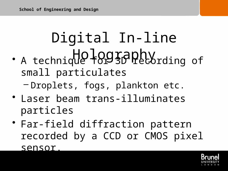
• A technique for 3D recording of small particulates– Droplets, fogs, plankton etc.
• Laser beam trans-illuminates particles• Far-field diffraction pattern recorded by a CCD or
CMOS pixel sensor.• Replay of each depth slice is computationally
intensive.

School of Engineering and Design
Theory of in-line holographyFrom: Hobson P.R. & Raouf A, Proceedings of SPIE. 1732 (1993) 663-676

School of Engineering and Design
Replay a digital in-line hologram1 . Numerically multiply the hologram by the reference wave (for our configuration of in-line holography the reference wave is 1+0i)
2. Take a Fourier transform
3. and multiply the result by a transfer function based on the Rayleigh-Sommerfeld equation.
4. An inverse Fourier transform gives the reconstructed image at one depth plane.

School of Engineering and Design
The in-focus objects, numerically replayed by computer
An in-line hologram of a test target, captured from a CCIR videocamera

School of Engineering and Design
Processing sequence• Digital hologram is read from file
• Image is zero-padded to power-of-two and set to complex by adding i0
• A forward 2D FFT is applied to the array
• A Transfer Function is applied, taking account of recording wavelength and desired image distance
• A reverse 2D FFT is performed
• The power spectrum is calculated and any zero-padding removed
• The reconstructed image is written to a file
School of Engineering and Design
Memory Allocation
HxW Float HxW Float HxW ComplexHxW Complex
Host GPU
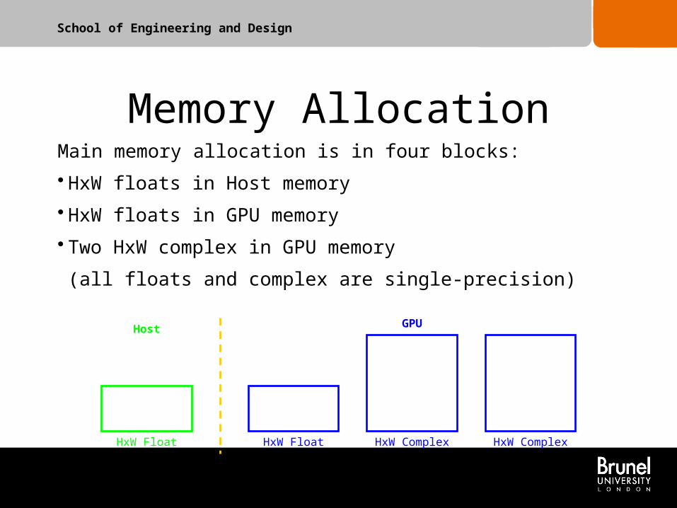
Main memory allocation is in four blocks:
• HxW floats in Host memory
• HxW floats in GPU memory
• Two HxW complex in GPU memory
(all floats and complex are single-precision)

School of Engineering and Design
File Read
HxW Float HxW Float HxW ComplexHxW Complex
Host GPU
Data are read from file into the host memory block as floats, possibly with zero-padding.
PGM::readPGMImage()
Input (float)

School of Engineering and Design
Data Transfer
HxW Float HxW Float HxW ComplexHxW Complex
Host GPU
Data are transferred into GPU memory.
cudaMemcpy()
Input (float) Input (float)

School of Engineering and Design
Forward FFT
HxW Float HxW Float HxW ComplexHxW Complex
Host GPU
A CUDA library real-to-complex FFT is performed, with the output placed in the second GPU buffer in packed form.
fftw_executeR2C()
Input (float) Input (float) FFT
(packed complex)
School of Engineering and Design
Unpack Data
HxW Float HxW Float HxW ComplexHxW Complex
Host GPU
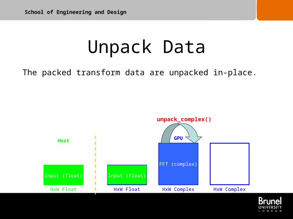
The packed transform data are unpacked in-place.
unpack_complex()
Input (float) Input (float)
FFT (complex)

School of Engineering and Design
Transform FFT
HxW Float HxW Float HxW ComplexHxW Complex
Host GPU
The Transfer Function for a given distance from the detector is applied to the FFT, taking into account wavelength and pixel size; the results are stored in the third GPU buffer.
applyTransferFunctionInFreqDomain()
Input (float) Input (float)
FFT (complex)
Transfer
Function
(complex)
School of Engineering and Design
Reverse FFT
HxW Float HxW Float HxW ComplexHxW Complex
Host GPU
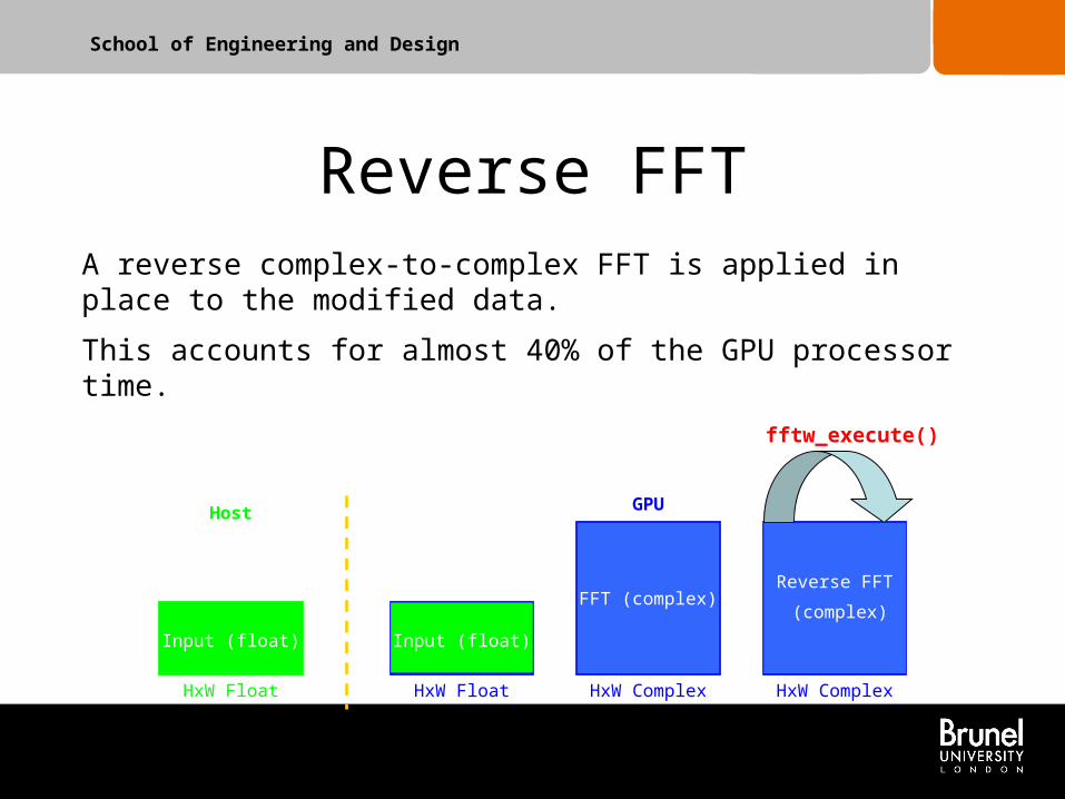
A reverse complex-to-complex FFT is applied in place to the modified data.
This accounts for almost 40% of the GPU processor time.
fftw_execute()
Input (float) Input (float)
FFT (complex)Reverse FFT
(complex)

School of Engineering and Design
Convert to Magnitudes
HxW Float HxW Float HxW ComplexHxW Complex
Host GPU
The magnitudes of the complex data are calculated and the resulting real data placed in the first GPU buffer. The cuPower16()function accounts for 18% of GPU processor time.
cuPower16()
Input (float)
FFT (complex)
Magnitude (float)
Reverse FFT
(complex)

School of Engineering and Design
Remove Zero-padding
HxW Float HxW Float HxW ComplexHxW Complex
Host GPU
If the data were zero-padded, the portion of the buffer corresponding to the initial pixels is copied back to the third buffer using a 2D memory-copy routine.
cudaMemcpy2D()
Input (float)
FFT (complex)
Magnitude (float)
Magnitude (float)

School of Engineering and Design
Normalise and Pack
HxW Float HxW Float HxW ComplexHxW Complex
Host GPU
The magnitude data has any constant offset removed and is then normalised to the required grey-scale level, the result being stored into the other buffer as unsigned 8- or 16-bit integers.
normpack()
Input (float)
FFT (complex)
Output (int) Output (int)

School of Engineering and Design
File Output: Transfer to Host
HxW Float HxW Float HxW ComplexHxW Complex
Host GPU
The packed integer data are now transferred back to the host.
cudaMemcpy()
FFT (complex)
Output (int) Output (int)Output (int)
School of Engineering and Design
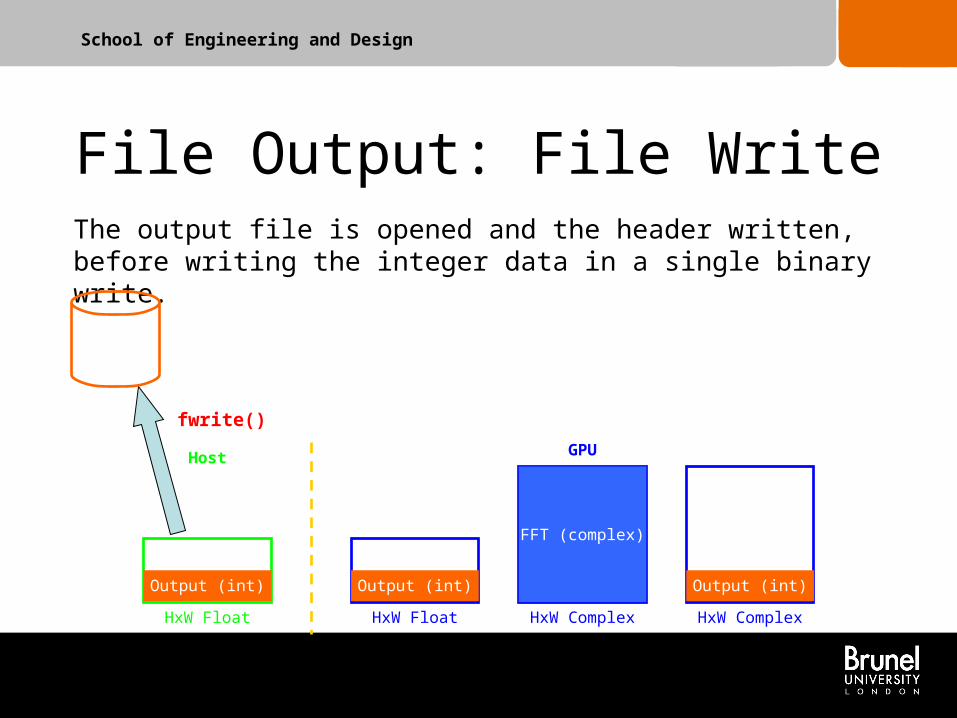
File Output: File Write
HxW Float HxW Float HxW ComplexHxW Complex
Host GPU
The output file is opened and the header written, before writing the integer data in a single binary write.
fwrite()
FFT (complex)
Output (int)Output (int) Output (int)

School of Engineering and Design
Open GL: Transfer to Display
HxW Float HxW Float HxW ComplexHxW Complex
Host GPU
The packed integer data are now transferred to a data buffer set up by the OpenGL compatability library for display.
cudaMemcpy()
FFT (complex)
Output (int) Output (int)
HxW Byte
Output (byte)

School of Engineering and Design
...and Loop!
HxW Float HxW Float HxW ComplexHxW Complex
Host GPU
If any more images are required at different distances, the programme continues looping from the transfer-function step (the forward FFT data remain in the second buffer); otherwise the buffers are deallocated and the programme terminated.
applyTransferFunctionInFreqDomain()
FFT (complex)
OutputN-1 (int)OutputN-1 (int)
Transfer
FunctionN
(complex)
School of Engineering and DesignFrom this

School of Engineering and Design
To this

School of Engineering and Design
Is a GPU a plug & play solution?Hologram: 2300x2500 px with 256 grey-levels, ASCII input, Times in cpu
seconds
CPU (8 core) GPU (Tesla S1070* (4GB) x3 gpu; 3.24 Tflops)
Read (ASCII) 2.55 2.52 (Serial)
Forward FFT 6.27 0.16 (Parallel – 2 host/device transfers)
Transfer Fn 1.20 1.17 (Serial)
Reverse FFT 6.06 0.19 (Parallel – 2 host/device transfers)
Write (ASCII) 1.37 1.40 (Serial)
Total 17.46 5.46
Simple-minded use of a powerful GPU with existing code is not sensible!
* S1070: 240 thread processors per gpu core, core clocked at 602 MHz

School of Engineering and Design
Code refactoring• Process several planes from one input and forward FFT to avoid expensive
read. Still requires transfer to/from device after serial transfer function calculation.
• Careful tuning of the transfer function and the (ASCII) write gave modest gains.
• After many code rearrangements, a way to parallelise inner loops of the transfer function was realised.
• This allows the results of the forward FFT to be kept in the GPU for the transfer function and reverse FFT, so no data movement needed until output stage.
• Transfer function time reduced to 0.08 s.• All calculations in single-precision.
Also parallelise the transfer function – the key improvement
School of Engineering and Design
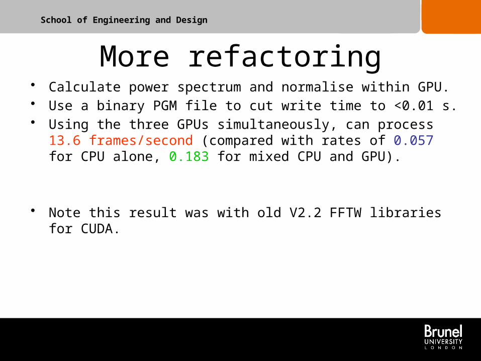
More refactoring• Calculate power spectrum and normalise within GPU.• Use a binary PGM file to cut write time to <0.01 s.• Using the three GPUs simultaneously, can process 13.6 frames/second
(compared with rates of 0.057 for CPU alone, 0.183 for mixed CPU and GPU).
• Note this result was with old V2.2 FFTW libraries for CUDA.
School of Engineering and Design
Real-world digital holography
Two clearly different user cases for hologram visualisation:
1) Expert user (e.g. a Marine Biologist) searches through video stream of replayed hologram depth slices looking for “interesting” objects. Very good use of the expert until she/he becomes bored!
2) Expert image-processing system searches through replayed hologram image slices looking for “objects”. Set of objects then sent to classifier.

School of Engineering and Design
GPU video replay of hologramsSome powerful NVidia GPU cards also have video outputs and there is an OpenGL compatability library available.
For human visualisation these are ideal since one can efficiently copy (using cudaMemcpy()) the replayed hologram to the video buffer and overall performance is not compromised.
Our latest results are:
For a Tesla C2050*; CUDA 4.0; Driver 285.03; in a Xeon 5620 @ 2.40 GHz, Ubuntu 10.10:
2300x3500 hologram, padded to 4Kx4K 15.1 frames/s2048x1389 hologram, padded to 2Kx2K 41.2 frames/s
* C2050: 448 thread processors in one gpu core, core clocked at 558 MHz
http://www.youtube.com/watch?v=WiE82RjqMzI

School of Engineering and Design
What about Grid computing?• Hobson & Watson* proposed grid computing for
silver-halide hologram image analysis (and digital hologram replay and analysis) nearly ten years ago.
• Digital hologram replay is trivially parallel.• Large scale production grids (and clouds) are
available.
* Hobson P.R. & Watson J. “The principles and practice of holographic recording of plankton” J. Opt. A: Pure Appl. Opt. 4 (2002) S34
School of Engineering and Design
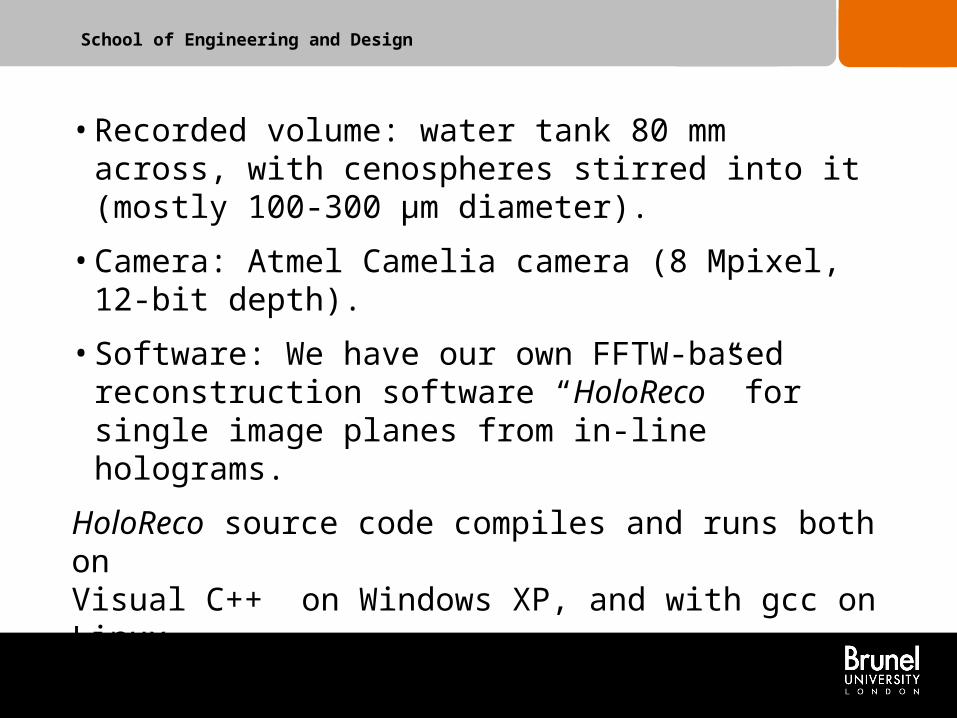
• Recorded volume: water tank 80 mm across, with cenospheres stirred into it (mostly 100-300 µm diameter).
• Camera: Atmel Camelia camera (8 Mpixel, 12-bit depth).
• Software: We have our own FFTW-based reconstruction software “HoloReco” for single image planes from in-line holograms.
HoloReco source code compiles and runs both on Visual C++ on Windows XP, and with gcc on Linux.
HoloReco is available from SourceForge.net
School of Engineering and Design
MethodWe submitted batches of Grid jobs each between 10 and 100
single slices to reconstruct the water tank with 0.1mm axial spacing (total 2200 slices = 91 GB), and looked at how long it took between starting the submission and the replayed images arriving back at the SE.
Each job loops, replaying a slice and immediately sending it back to the SE.
Compare this with replaying the slices sequentially on a single cpu.
Note: this grid performance data was shown at “EOS Blue Photonics”, Aberdeen, UK in August 2009.
School of Engineering and Design
0
500
1000
1500
2000
2500
00:00:00 02:24:00 04:48:00 07:12:00 09:36:00 12:00:00
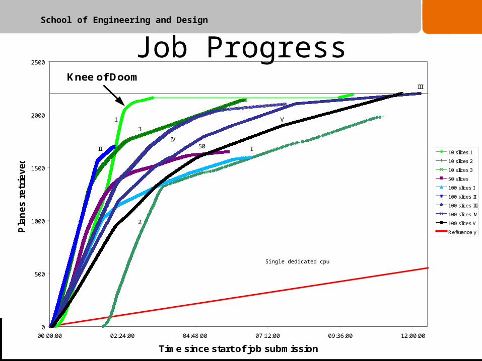
Time since start of job submission
Pla
ne
s r
etr
iev
ed
10 slices 1
10 slices 2
10 slices 3
50 slices
100 slices I
100 slices II
100 slices III
100 slices IV
100 slices V
Reference y
1
2
3
50 III
III
IV
V
Knee of Doom
Single dedicated cpu
Job Progress

School of Engineering and Design
Speed-up in practice
0.0
5.0
10.0
15.0
20.0
50% 70% 90% 100%
Percentage of 2200 slices completed
Ave
rage
spe
ed-u
p fa
ctor
10 slices per job
100 slices per job

School of Engineering and Design
Recent results with grid
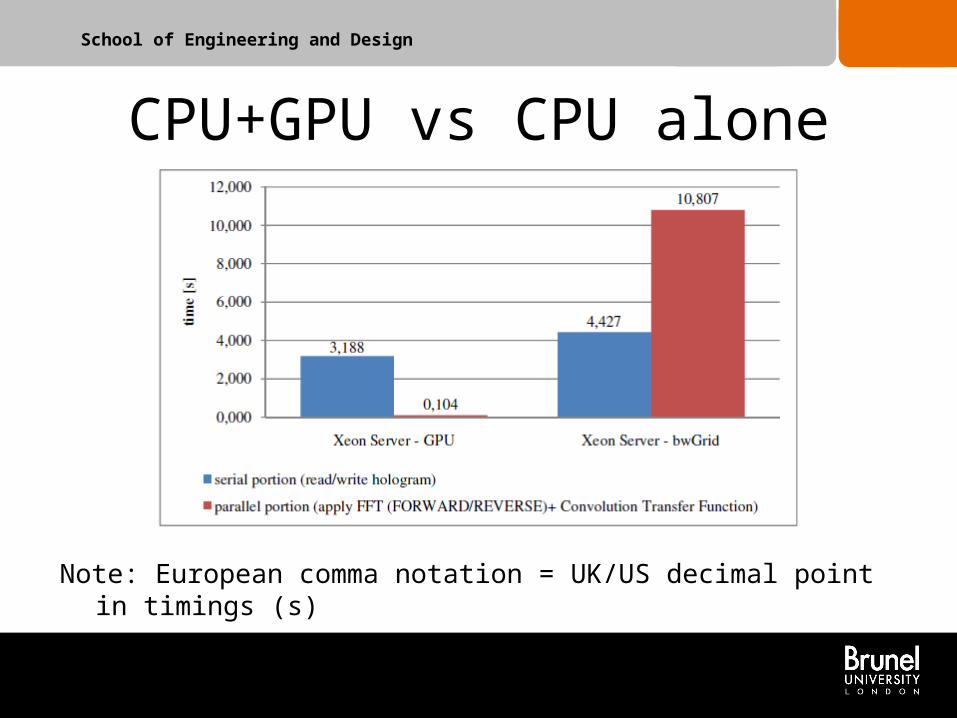
• A second comparison, using “bwGrid” in Esslingen and an nVidia Tesla C1060* at Brunel both using 4-core Xeon X5550 host processors has been carried out in 2011.
• In these tests we are writing to local storage the replayed images (no video).
* C1060: 240 thread processors in one gpu core, core clocked at 602 MHz
School of Engineering and Design
CPU+GPU vs CPU alone
Note: European comma notation = UK/US decimal point in timings (s)

School of Engineering and Design
Calculated values for sequential processing.
Measured values for other categories.

School of Engineering and Design
Conclusions - 1• For digital hologram scanning by human expert with
highly optimised code current GPU are clearly the hardware of choice.
• We now have a highly GPU optimised version (> 200 times faster) of HoloReco, with another ~10% to be gained from further refactoring.
• Grids suffer from both non-deterministic return time/slice ordering of data and from the real possibility of non-completion of all depth slices.

School of Engineering and Design
Conclusions - 2• For the complete automation of all processing
(hologram replay to classified object) the case is less clear. 3D image processing (IP) requires many depth-slices to be available simultaneously on a node.
• It is not clear that existing IP software libraries used on conventional x86 systems will be ported efficiently to GPU architecture (legacy code issue).
• Possibly a hybrid “GPU + Grid/Cloud” approach is currently the optimum.

School of Engineering and Design
Acknowledgements• Access to the S1070 GPU system was generously
provided by Viglen (UK).• GridPP and London Tier 2 institutes for UK grid
resources supporting the LTWO VO.• HS Esslingen for “bwGrid” resources in Germany.• Sven Sander for running jobs and providing data using
bwGrid.
Recommended