SiF 2020 – The 11th International Conference on Structures in Fire
The University of Queensland, Brisbane, Australia, 30th November - 2nd December, 2020
PROBABILISTIC MODELS FOR THERMAL PROPERTIES OF CONCRETE
Balša Jovanović1, Negar Elhami Khorasani2, Thomas Thienpont3, Ranjit Kumar Chaudhary4, Ruben Van
Coile5
ABSTRACT
Thermal conductivity and specific heat of concrete are highly influential parameters for the heat transfer
into the material during fire exposure. Reviewing the available literature has shown that there is a large
scatter in the data for these thermal parameters. To quantify that uncertainty, novel probabilistic models for
thermal conductivity and specific heat of concrete at elevated temperatures are developed.
Analysis of available experimental data indicates that a temperature-dependent Gamma distribution can
be recommended for both thermal properties. Closed-form equations for the temperature-dependent mean
and standard deviation are derived. Thus, for both the thermal conductivity and the specific heat, a
continuous probability distribution as a function of temperature is obtained, which can be easily
implemented in numerical simulations. Using the example of the probabilistic analysis of a simply
supported concrete slab exposed to the standard fire, the models are compared with the commonly used
deterministic representation of the thermal properties. It is shown that the calculated probabilities of
failure using the deterministic models are an order of magnitude lower and therefore
unconservative. This analysis suggests that accounting for the uncertainty in thermal properties for
concrete slabs can have a significant effect on evaluating the safety and therefore should not be ignored
in cases of high importance.
Keywords: Fire; specific heat; thermal conductivity; uncertainty; failure probability
1 INTRODUCTION
Fire is a rare event that can have a significant negative impact on people’s safety. Luckily many fires are
extinguished or suppressed early on by the occupants of the building or active measures (e.g. sprinklers).
However, when fires progress beyond this level, they can cause serious damage to the structure. The effects
of these, often referred to as ‘structurally significant’, fires are analysed in structural fire engineering (SFE).
The main task of SFE is to produce a design solution that provides an adequate safety level, more precisely
a solution with the failure probability below an explicit or implicit acceptable value.
1 Corresponding author, Ghent University e-mail: [email protected], ORCID: https://orcid.org/0000-0001-5200-58482 University at Buffaloe-mail: [email protected], ORCID: https://orcid.org/0000-0003-3228-00973 Ghent Universitye-mail: [email protected], ORCID: https://orcid.org/0000-0003-1466-33774 Ghent Universitye-mail: [email protected], ORCID: https://orcid.org/0000-0002-1104-5859 5 Ghent University
e-mail: [email protected], ORCID: https://orcid.org/0000-0002-9715-6786
https://doi.org/10.14264/363ff91
342

In most design situations, the combination of prescribed fire resistance ratings and standardized calculation
methods is sufficient to prove that the structure has an adequately low, although unquantified, failure
probability. In special cases of high importance, however, adequate safety needs to be demonstrated
explicitly. In those situations, (semi-)probabilistic calculations are required which directly take into account
the stochastic nature of the input parameters. Even though the appropriate probabilistic models for some of
these input variables are well-defined, others are often regarded as deterministic due to the lack of the
appropriate models.
Probabilistic structural fire engineering (PSFE) is traditionally conducted using a large number of
calculations with varying parameters and using numerical simulations. As the probabilistic approach is
much more developed in classical structural engineering, the stochastic description of a large number of
input variables needed for the structural analysis is well defined. This involves the geometry [1], loads [2]
and material strength at ambient and elevated temperatures [3]. However, concerning the heat transfer part
of the calculation, there is not much information available on the stochastic description of needed inputs.
Heat transfer has three modes: convection, radiation, and conduction. When conducting the heat transfer
analysis for the temperature within structural members, the first two modes can be considered as a boundary
condition and the last, conduction, as the main mode of temperature propagation through the concrete
element. Conduction represents the diffusion of thermal energy (heat) within the material.
Thermal conductivity, k describes the material’s ability to conduct heat, and specific heat, cp represents the
amount of energy needed to heat up a unit mass of the material by a unit temperature. Both of these
properties are highly material and temperature dependant. Their influence on the thermal gradient within
an element is defined by Fourier’s law of (1D) conduction:
𝜕𝑇
𝜕𝑡=
𝑘
𝜌𝑐𝑝∇2𝑇 (1)
where 𝜕𝑇
𝜕𝑡 represents the change of temperature with time, 𝒌 [ 𝑾𝒎∙𝑲] is the thermal conductivity, 𝒄𝒑 [
𝑱
𝒌𝒈∙𝑲] is
the specific heat and 𝜌 is the material density.
The heat transfer analysis in SFE in its essence represents the numerical solution of the multidimensional
version of equation (1). The most commonly used approach is to use the deterministic models for these
thermal properties as provided in guidance documents. For concrete, some of the most widely used models
are those presented in Eurocode [4]. Thermal conductivity is defined by two limits (upper and lower) that
are given as quadratic functions of the temperature 𝑇:
𝑘𝑢𝑝𝑝𝑒𝑟 = 2.00 − 0.2451 ∙ (𝑇/100) + 0.0107 ∙ (𝑇/100)2 for 20°𝐶 ≤ 𝑇 ≤ 1200°𝐶 (2)
𝑘𝑙𝑜𝑤𝑒𝑟 = 1.36 − 0.1360 ∙ (𝑇/100) + 0.0057 ∙ (𝑇/100)2 for 20°𝐶 ≤ 𝑇 ≤ 1200°𝐶 (3)
where the choice of the exact value between these two limits is left to the user, but the lower values are
recommended
On the other hand, specific heat is given as a single piecewise function:
𝑐𝑝 = 0.9 for 20°𝐶 ≤ 𝑇 ≤ 100°𝐶
𝑐𝑝 = 0.9 + (𝑇 − 100)/1000 for 100°𝐶 ≤ 𝑇 ≤ 200°𝐶 (4)
𝑐𝑝 = 1.0 + (𝑇 − 200)/2000 for 200°𝐶 ≤ 𝑇 ≤ 400°𝐶
𝑐𝑝 = 1.1 for 400°𝐶 ≤ 𝑇 ≤ 1200°𝐶
343
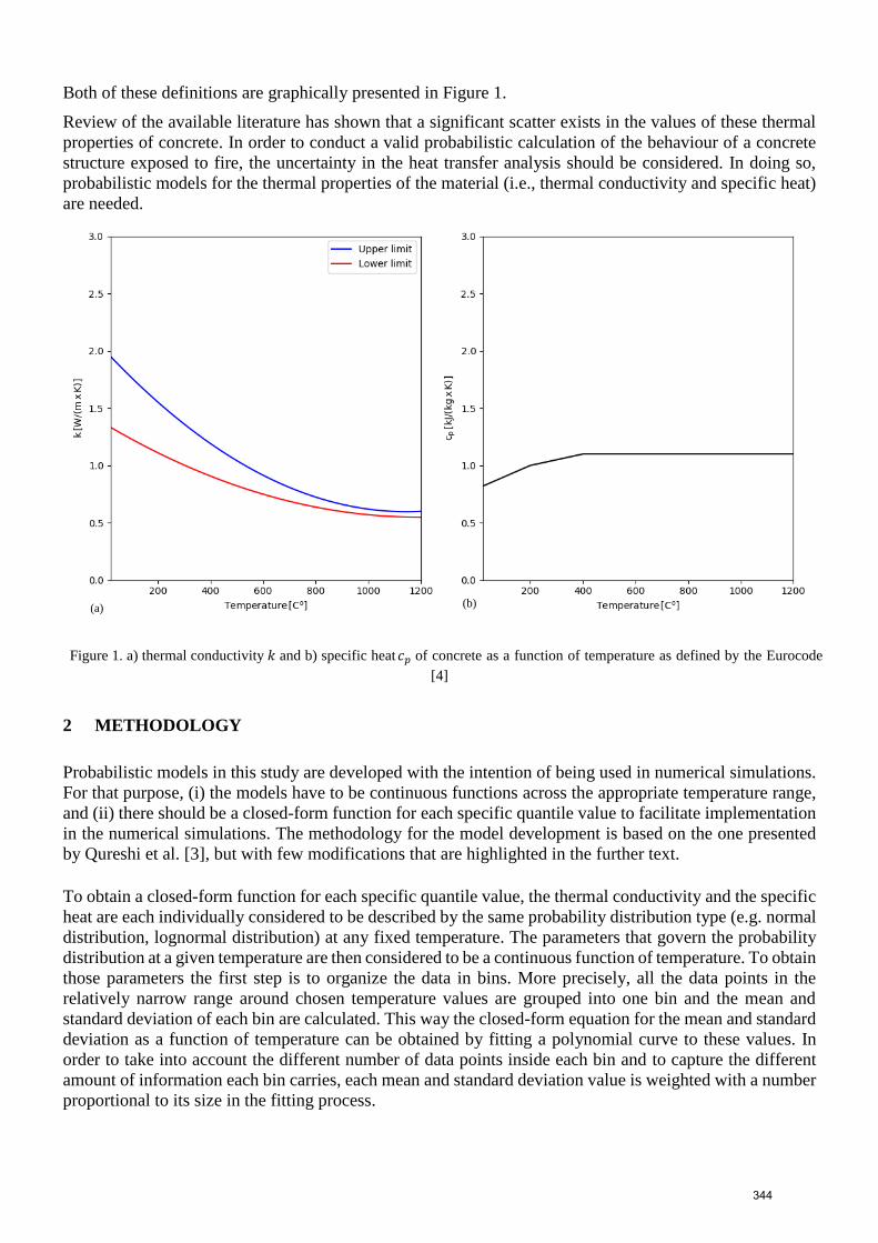
Both of these definitions are graphically presented in Figure 1.
Review of the available literature has shown that a significant scatter exists in the values of these thermal
properties of concrete. In order to conduct a valid probabilistic calculation of the behaviour of a concrete
structure exposed to fire, the uncertainty in the heat transfer analysis should be considered. In doing so,
probabilistic models for the thermal properties of the material (i.e., thermal conductivity and specific heat)
are needed.
Figure 1. a) thermal conductivity 𝑘 and b) specific heat 𝑐𝑝 of concrete as a function of temperature as defined by the Eurocode [4]
2 METHODOLOGY
Probabilistic models in this study are developed with the intention of being used in numerical simulations.
For that purpose, (i) the models have to be continuous functions across the appropriate temperature range,
and (ii) there should be a closed-form function for each specific quantile value to facilitate implementation
in the numerical simulations. The methodology for the model development is based on the one presented
by Qureshi et al. [3], but with few modifications that are highlighted in the further text.
To obtain a closed-form function for each specific quantile value, the thermal conductivity and the specific
heat are each individually considered to be described by the same probability distribution type (e.g. normal
distribution, lognormal distribution) at any fixed temperature. The parameters that govern the probability
distribution at a given temperature are then considered to be a continuous function of temperature. To obtain
those parameters the first step is to organize the data in bins. More precisely, all the data points in the
relatively narrow range around chosen temperature values are grouped into one bin and the mean and
standard deviation of each bin are calculated. This way the closed-form equation for the mean and standard
deviation as a function of temperature can be obtained by fitting a polynomial curve to these values. In
order to take into account the different number of data points inside each bin and to capture the different
amount of information each bin carries, each mean and standard deviation value is weighted with a number
proportional to its size in the fitting process.
(a) (b)
344

After both the mean value and standard deviation are fitted in the form of a polynomial function, the
appropriate probability distribution must be determined. This is done based on the Akaike Information
Criteria (AIC) [5]:
𝐴𝐼𝐶 = 2𝑚 − 2ln(𝐿) (5)
where 𝑚 represents the number of estimated parameters in the model and 𝐿 is the likelihood of the model
for the given data. It must be noted that the AIC value can only be used as a comparative measure, more
precisely, a single absolute value of AIC on its own does not contain any useful information. It can only be
used to compare two or more models in a way that the model with the lowest AIC value represents the best
fit.
The procedure to find the most appropriate distribution is as follows: Firstly, for each data point, the
corresponding model mean and the standard deviation are calculated, based on the data point’s temperature
and the previously fitted polynomial functions. Based on those two values a specific theoretical distribution
is defined and the likelihood of the data point is calculated. Lastly, the total likelihood is calculated by
multiplying the values for each data point, and the AIC for a specific theoretical distribution is then obtained
through (5). Using all the AIC values the best distribution is chosen.
It should be highlighted that even though the methodology described here is based on the work presented
in [3] it has a couple of distinctive differences. First, the choice of adequate theoretical distribution is done
more holistically, using the AIC for every data point based on the fitted curves for the governing parameters,
instead of fitting the distribution for each bin separately, summing the AIC for each bin and then fitting a
curve on the parameters. As its direct consequence, the second difference is fitting of the polynomial
functions on mean and standard deviation values instead of the specific chosen distribution’s parameters.
The main advantage of this modified approach is that the best candidate distribution is chosen based on the
final model and all the data points instead of only the data in the bins.
3 RESULTS AND DISCUSSION
The temperature range of 20 − 1200°𝐶 is chosen based on three factors, firstly the available data for
constructing the model, secondly the fact that damage to the concrete at temperatures higher than 1000°𝐶
is large enough that it loses all of its mechanical properties, and finally the range of the commonly used
Eurocode models.
Based on the available literature data, it is evident that the thermal properties differ significantly based on
the type of concrete, whether its lightweight, normal strength (NSC) or high strength concrete (HSC). The
focus in this paper is on the NSC as it is the most commonly used type. When considering the type of
aggregate used in the concrete, it is decided to not make the distinction between siliceous and calcareous,
in order to be in sync with the widely used Eurocode models for thermal properties [4].
Data needed for the creation of the models have been collected from the literature. Some data was found as
tabulated values, but the majority had to be extrapolated from figures. The thermal conductivity dataset
collected in this study consists of 382 points taken from 12 sources [6–17]. On the other hand, the specific
heat data consists of 343 points taken from 9 sources [6, 8, 9, 12, 14–16, 18, 19].
345
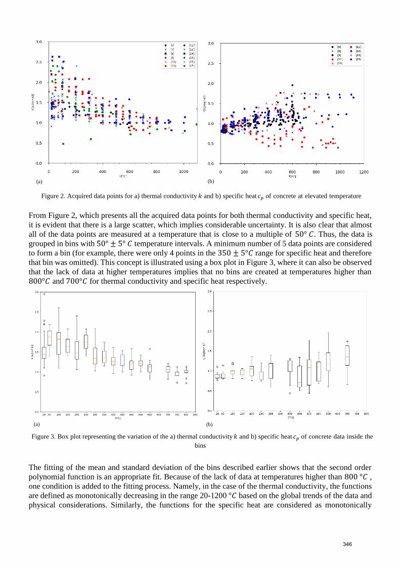
Figure 2. Acquired data points for a) thermal conductivity 𝑘 and b) specific heat 𝑐𝑝 of concrete at elevated temperature
From Figure 2, which presents all the acquired data points for both thermal conductivity and specific heat,
it is evident that there is a large scatter, which implies considerable uncertainty. It is also clear that almost
all of the data points are measured at a temperature that is close to a multiple of 50°𝐶. Thus, the data is
grouped in bins with 50° ± 5°𝐶 temperature intervals. A minimum number of 5 data points are considered
to form a bin (for example, there were only 4 points in the 350 ± 5°𝐶 range for specific heat and therefore
that bin was omitted). This concept is illustrated using a box plot in Figure 3, where it can also be observed
that the lack of data at higher temperatures implies that no bins are created at temperatures higher than
800°𝐶 and 700°𝐶 for thermal conductivity and specific heat respectively.
Figure 3. Box plot representing the variation of the a) thermal conductivity 𝑘 and b) specific heat 𝑐𝑝 of concrete data inside the bins
The fitting of the mean and standard deviation of the bins described earlier shows that the second order
polynomial function is an appropriate fit. Because of the lack of data at temperatures higher than 800°𝐶 ,
one condition is added to the fitting process. Namely, in the case of the thermal conductivity, the functions
are defined as monotonically decreasing in the range 20-1200°𝐶 based on the global trends of the data and
physical considerations. Similarly, the functions for the specific heat are considered as monotonically
(a) (b)
(a) (b)
346

increasing in the same domain. The resulting equations are graphically presented in Figure 4 and are the
following:
𝑚𝑒𝑎𝑛𝑘 = 6.627 × 10⁻⁷ × 𝑇2 − 1.458 ×10⁻³ × 𝑇 + 1.772 (6)
𝑠𝑡𝑑𝑘 = 3.139 ×10⁻⁷ × 𝑇2 − 0.691 × 10⁻³ × 𝑇 + 0.434 (7)
𝑚𝑒𝑎𝑛𝑐𝑝 =−2.953 ×10⁻⁷ × 𝑇2 + 6.498 × 10⁻⁴ × 𝑇 + 0.872 (8)
𝑠𝑡𝑑𝑐𝑝 = −3.500 × 10⁻⁷ × 𝑇2 + 7.700 ×10⁻⁴ × 𝑇 + 0.042 (9)
Figure 4. Polynomial function fit for the mean and standard deviation values for a) thermal conductivity 𝑘 and b) specific heat
𝑐𝑝 of concrete
Numerous two parameter theoretical distributions have been fitted in order to find the most adequate
one for the models. More precisely, the fitted distributions were: Normal, Lognormal, Gamma, Gumbel,
Beta44, Weibull, Inverse Gaussian, Logistic, Log-logistic, Rican, Nakagami and Birnbaum Saunders.
Figure 5 shows the AIC values obtained for different distributions (for clarity only the five best fits are
presented, as the values for the others were an order of magnitude larger). Both in the case of thermal
conductivity and specific heat, the best fits (i.e., the lowest AIC score) are obtained by Normal and Gamma
distributions. From the two, the Gamma distribution is chosen given that, on the contrary to the Normal
distribution, it has zero probability for negative values (which are theoretically impossible for these thermal
properties).
Figure 6 presents the obtained models alongside with the data points and Eurocode models. In the case of
the specific heat, it can be seen that the 50% quantile values are close to those prescribed in Eurocode,
however, that is not the case for thermal conductivity where the overlap between the two is minimal,
especially at higher temperatures. Also, it can be seen that even though the data points for temperatures
higher than 800°𝐶 were not used for the fiting of polygonal functions due to the lack of data, the overall
model behaviour describes them relatively well.
(a) (b)
347

Figure 5. Akaike information criteria (AIC) comparison of a few theoretical distributions for a) thermal conductivity and b)
specific heat of concrete
For the specific heat, the Eurocode [4] recommends an additional peak between 100°𝐶 and 200°𝐶, as a
function of the moisture content, to take into account the moisture inside the concrete and the needed energy
for moisture evaporation. Due to the great similarities of the 50% quantile curve, the same approach with
the same values is recommended when using the probabilistic model for the specific heat of concrete. More
precisely, the same moisture peak values are added to the specific heat curve for the desired quantile value.
Even though the models do not provide a direct closed-form equation for any quantile value, the needed
value can be easily calculated in two steps. Firstly the mean and the standard deviation are calculated for a
given temperature and then based on the two calculated values and the desired quantile, the thermal property
is evaluated using the well-known equations defining the Gamma distribution.
Figure 6. Probabilistic models for (a) thermal conductivity and (b) specific heat of concrete at elevated temperatures: 5%,
50%, and 95% quantiles, together with the model from Eurocode and the raw data.
4 EXAMPLE
An example of a simply supported concrete slab exposed to the standard fire will be used to demonstrate
the influence of stochasticity in concrete thermal properties on the probability of failure. This example, but
(a) (b)
(a) (b)
348

with deterministic thermal properties, in accordance with the Eurocode, was used in [20]. The slab in
question is exposed to the fire only on the bottom side, while the top side is subjected to the ambient
conditions. Thus, for the considered slab thickness, it is safe to assume that the temperatures on the top (i.e.,
the compression side) will not achieve values high enough to cause considerable strength reduction. For
those reasons, it is justifiable to use the following equation to calculate the resisting moment of the slab,
𝑀𝑅:
𝑀𝑅 = 𝑘𝑓𝑦 ∙ 𝑓𝑦,20 ∙ 𝐴𝑆 ∙ (ℎ −∅2⁄ − 𝑐) −
(𝑘𝑓𝑦 ∙𝑓𝑦,20∙𝐴𝑆)2
2∙𝑏∙𝑓𝑐(10)
where 𝑏 is the slab width (taken as 1 m) and all the other parameters, along with their distributions, are
presented in Table 1.
A probabilistic analysis based on 104 Latin Hypercube Samples (LHS) is conducted in three parts: (i) first
the heat transfer analysis using finite difference method and newly presented probabilistic models for
thermal conductivity and specific heat are conducted in order to obtain the temperature distribution inside
the slab; (ii) next, taking into account the temperature of the reinforcements inside the slab and Eqn. (10),
the moment capacity of the slab is calculated; and (iii) finally, the probability of failure is calculated based
on the loads and model uncertainties presented in Table 2 and using the limit state equation:
𝑍 = 𝑅 − 𝐸 = 𝐾𝑅 ∙ 𝑀𝑅 − 𝐾𝐸 ∙ (𝐺 + 𝑄) (11)
Figure 7 (a) shows the results of the heat transfer analysis, specifically the temperature gradient inside the
slab after 120 and 180 minutes of standard fire exposure. In the figure, also the temperature gradient
obtained using the Eurocode equations (lower limit) for thermal properties is presented. The most notable
observation is that the temperatures are higher when calculated using the probabilistic models. The
Eurocode temperature gradient is on the level of the 5% quantile of the probabilistic model for both fire
exposure times, and only close to the top surface of the slab, where the temperature is close to ambient
condition, does the Eurocode temperature gradient come closer to the median results obtained with the
probabilistic model.
Table 1. Stochastic input parameters used for the moment capacity calculation
Parameter Distribution Mean μ Standard deviation σ Ref
20°C concrete compressive strength, 𝑓𝑐,20 [MPa] Lognormal 42.9 (𝑓𝑐𝑘 = 30𝑀𝑃𝑎) 6.44 [21]
20°C reinforcement yield strength, 𝑓𝑦,20 [MPa] - 560 (𝑓𝑦𝑘 = 500𝑀𝑃𝑎) - -
Steel yield stress retention factor, 𝑘𝑓𝑦[-] Lognormal Temperature dependent Temperature dependent [3]
Reinforcement area, 𝐴𝑆[𝑚𝑚2/𝑚] Normal 785 16 [21]
Reinforcement diameter, ∅[𝑚𝑚] - 10 - -
Slab height, ℎ[𝑚] - 0.2 - -
Concrete cover, 𝑐 [mm] Beta [μ ±3σ] 30+5 = 35 5 [1]
Figure 7 (b) shows the Probability Density Function (PDF) of moment capacity of the slab. It can be seen
that an analysis using the Eurocode thermal properties overestimates the slab capacity compared to an
analysis using the probabilistic models for thermal properties. This indeed can be explained by the higher
temperatures in the reinforcement. The difference is even better illustrated in Figure 8, which shows the
Cumulative Distribution Function (CDF) of the limit state from the Eqn. 11. The CDF value at 0𝑘𝑁𝑚
represents the probability of failure. Probabilites of failure in the case where the probabilistic model for the
349

thermal properties is used are an order of magnitude higher compared to those obtained using the Eurocode
thermal models, more precisely 2.82 ∙ 10−4 vs 2.37 ∙ 10−5 and 7.32 ∙ 10−2 vs 3.07 ∙ 10−3 for 120 and 180
min respectively. This difference in the probability of reaching the limit state illustrates how important it is
to take into account the uncertainties in the thermal properties of concrete, especially since using the
deterministic model is unconservative.
Figure 7. a) Temperature gradient inside of the concrete slab after 120 and 180 minutes of standard fire exposure at the
bottom side, b) PDFs of the slab bending capacity calculated using the probabilistic and deterministic models for the thermal
properties of concrete
Table 2. Stochastic input parameters used for calculation for the probability of failure
Parameter Distribution Mean μ Standard deviation σ Ref
Dead load, 𝐺[𝑘𝑁𝑚] Normal 15 1.5 [2]
Live load, Q[𝑘𝑁/𝑚2] Gamma 1.875 1.78 [2]
Model uncertainty for the load effect, 𝐾𝐸[-] Lognormal 1 0.1 [2]
Model uncertainty for the resistance effect, 𝐾𝑅[-] Lognormal 1 0.15 [2]
Figure 8 CDFs of the limit state calculated using the probabilistic and deterministic models for the thermal properties of
concrete
(a) (b)
350

5 CONCLUSION
Novel probabilistic models for thermal conductivity and specific heat of concrete are developed. The
motivation for this study is the large uncertainty in the thermal properties of concrete that is evident from
the large scatter in data reported in the literature. The models provide an efficient way to define the value
of the thermal property at a specific temperature for the required quantile value, which is highly suitable
for numerical simulations.
Models for both thermal parameters are defined using two steps. First, the mean and standard deviation are
calculated for a specific temperature using Eqn. (6)-(9). Afterwards, the thermal property value can be
generated based on the mean, standard deviation and the specified quantile value using the Gamma
distribution.
In the case of the specific heat, the median, 50% quantile, values are similar to those prescribed in Eurocode,
but the overall model still shows considerable variation. For thermal conductivity, however, the values are
much larger and show a relatively small overlap with the Eurocode models. The influence of such
differences is demonstrated using the probabilistic structural fire engineering analysis of a simply supported
concrete slab. It was shown that a considerable difference in the temperature gradient, moment capacity
and finally probability of failure could be expected when using the developed models as opposed to existing
deterministic relationships.
Using the traditional deterministic models for thermal properties is justified for simple design situations,
but the uncertainty of the thermal properties values cannot be neglected for special cases where the
probabilistic calculations are needed, as traditional models could lead to unconservative results.
REFERENCES
1. JCSS, (2001). Probabilistic Model Code. Part 3.10 Dimensions. Joint Committee on Structural Safety
2. Jovanović, B, Van Coile, R, Hopkin, D, Elhami Khorasani, N, Lange, D, Gernay, T, (2020). Review of
Current Practice in Probabilistic Structural Fire Engineering: Permanent and Live Load Modelling. Fire
Technol. https://doi.org/10.1007/s10694-020-01005-w
3. Qureshi, R, Ni, S, Elhami Khorasani, N, Van Coile, R, Hopkin, D, Gernay, T, (2020). Probabilistic models
for temperature dependent strength of steel and concrete. Journal of Structural Engineering 146:04020102.
https://doi.org/10.1061/(asce)st.1943-541x.0002621
4. CEN, (2004). EN 1992-1-2:2004: Eurocode 2: Design of concrete structures - Part 1-2: General rules.
Structural fire design. European Standard
5. Akaike, H, (1974). A new look at the statistical model identification. IEEE Transactions on Automatic Control
19:716–723
6. Harmathy, T, Allen, L, (1973). Thermal properties of selected masonry unit concretes. Journal of The
American Concrete Institute 70:132–142
7. Harada, T, Takeda, J, Yamane, S, Furumura, F, (1972). Strength, Elasticity and Thermal Properties of
Concrete Subjected to Elevated Temperatures. ACI Structural Journal 34:377–406
8. Schneider, U, (1988). Concrete at high temperatures - A general review. Fire Safety Journal 13:55–68.
https://doi.org/10.1016/0379-7112(88)90033-1
9. Adl-Zarrabi, B, Boström, L, Wickström, U, (2006). Using the TPS method for determining the thermal
properties of concrete and wood at elevated temperature. Fire and Materials 30:359–369.
https://doi.org/10.1002/fam.915
10. Banerjee, DK, (2016). An analytical approach for estimating uncertainty in measured temperatures of concrete
slab during fire. Fire Safety Journal 82:30–36. https://doi.org/10.1016/j.firesaf.2016.03.005
11. Kodur, KR, Dwaikat, MMS, Dwaikat, MB, (2009). High-temperature properties of concrete for fire resistance
modeling of structures. ACI Materials Journal 106:390
12. Shin, K-Y, Kim, S-B, Kim, J-H, Chung, M, Jung, P-S, (2002). Thermophysical Properties and Transient Heat
Transfer of Concrete at elevated temperature. Nuclear Engineering and Design 212:233–241
13. Anderberg, Y, (1976). Fire-exposed concrete structures. An experimental and theoretical study. Bull Div
351

Struct Mech Concr Constr
14. Lie, TT, Kodur, VKR, (1995). Thermal properties of fibre-reinforced concrete at elevated temperatures.
National Research Council Canada, Institute for Research in Construction
15. Kakae, N, Miyamoto, K, Momma, T, Sawada, S, Kumagai, H, Ohga, Y, Hirai, H, Abiru, T, (2017). Physical
and thermal properties of concrete subjected to high temperature. Journal of Advanced Concrete Technology
15:190–212. https://doi.org/10.3151/jact.15.190
16. Hu, XF, Lie, TT, Polomark, GM, Maclaurin, JW, (1993). Thermal properties of building materials at elevated
temperatures. Intern report/National Res Counc Canada, Inst Res Constr no 643
17. Marechal, J, (1972). Conductivity and Thermal Expansion Coefficients of Concrete as a Function of
Temperature and Humidty. Special Publication 34:1047--1058
18. T.T. Lie, (1980). Structural Fire Protection
19. Naus, DJ, (2006). The effect of elevated temperature on concrete materials and structures-A literature review.
Oak Ridge National Laboratory (United States)
20. Thienpont, T, Van Coile, R, De Corte, W, Caspeele, R, (2019). Determining a global resistance factor for
simply supported fire exposed RC slabs. In: Concrete : innovations in materials, design and structures: fib
Symposium 2019. pp 2191–2197
21. Holický, M, Sýkora, M, (2010). Stochastic models in analysis of structural reliability. In: International
symposium on stochastic models in reliability engineering, life sciences and operation management, Beer
Sheva, Israel
352
Recommended