Chi

A prospective study for probabilistic approach of thermal fatigue in mixing tees

V. Radu E. Paffumi N. Taylor K.-F. Nilsson

EUR 23570 EN - 2009

The Institute for Energy provides scientific and technical support for the conception, development, implementation and monitoring of community policies related to energy. Special emphasis is given to the security of energy supply and to sustainable and safe energy production. European Commission Joint Research Centre Institute for Energy Contact information Address: E. Paffumi E-mail: elena.paffumi@jrc.nl Tel.: +31 224 565082 Fax: +31 224 565641 http://ie.jrc.ec.europa.eu http://www.jrc.ec.europa.eu Legal Notice Neither the European Commission nor any person acting on behalf of the Commission is responsible for the use which might be made of this publication. A great deal of additional information on the European Union is available on the Internet. It can be accessed through the Europa server http://europa.eu/ JRC 48003 EUR 23570 EN ISSN 1018-5593 Luxembourg: Office for Official Publications of the European Communities © European Communities, 2009 Reproduction is authorised provided the source is acknowledged Printed in The Netherlands

2

A prospective study for probabilistic approach of thermal fatigue in mixing tees

V. Radu E. Paffumi N. Taylor K.-F. Nilsson

3

Contents

1. INTRODUCTION................................................................................................................................................... 3

2. BACKGROUND ON THE STRUCTURAL RELIABILITY METHOD .......................................................... 4

2.1 Limit States............................................................................................................................................. 4 2.2 Probabilistic approach and assessment procedure................................................................................ 5 2.3 Objective of structural reliability analysis ............................................................................................. 6 2.4 Structural reliability theory.................................................................................................................... 7

3. PROBABILITY ANALYSIS................................................................................................................................ 10

4. PROSPECTIVE STUDY FOR PROBABILISTIC ANALYSIS APPLIED TO CIVAUX 1 CASE .............. 12

4.1 Case description................................................................................................................................... 12 4.2 Failure mode and function ................................................................................................................... 14 4.3 Input parameters and distributions ...................................................................................................... 16 Crack size distribution................................................................................................................................ 16 Paris law parameters distribution ............................................................................................................... 17 4.4 Analysis and discussion........................................................................................................................ 18

5. CONCLUSIONS ................................................................................................................................................... 21

GLOSSARY............................................................................................................................................................... 23

APPENDIX: THE CDFS AND PDFS USED FOR PROBABILISTIC FATIGUE APPROACH ..................... 25

a) Normal distribution (Gauss distribution) ............................................................................................... 25 b) Exponential distribution......................................................................................................................... 25 c) Log-normal distribution ......................................................................................................................... 26 d) Empirical cumulative distribution.......................................................................................................... 26

FIGURES................................................................................................................................................................... 28

REFERENCES.......................................................................................................................................................... 34

4

1. INTRODUCTION

The cracking in the NPP piping system remains a main concern and deterministic

structural integrity assessment need to be combined with probabilistic approaches in

order to consider uncertainties in material, environment and loading properties. The

deterministic fracture mechanics approach for a defined problem can be transformed to

a probabilistic approach by considering some of the inputs to be random variables.

Candidates as random variables include initial crack locations and size (depth and

length), fracture toughness, subcritical crack growth characteristics, stress levels,

environmental effects, etc. In addition, the effects of inspection can be included through

their influence on crack detection, sizing and repair. The characterization of the

statistical distribution of fracture mechanics random variables consists of collecting

information from testing and literature and, also, characterizing its scatter by selection

the type of distribution and the parameters of the distribution. The analytical

developments could be sustained by finite element analyses (FEA) performed to

provide input stress loadings.

Thermal fatigue has caused through-wall cracking and leakage in BWR and PWR plants

from low-cycle and high-cycle thermal fatigue. Experience [1], [2] suggests that service-

induced fatigue in operating plants are caused primarily by thermal stratification or hot-

cold water mixing conditions, such as thermal striping, and cyclic turbulent mixing not

analyzed in the original plant designs. The problem of thermal fatigue in mixing areas

arises in pipes where turbulent mixing or vortices produce rapid fluid temperature

fluctuations with random frequencies. These loadings consist of many cycles with the

cyclic boundary conditions changing quickly, causing cracks to initiate and grow at

multiple locations on the inside surface of the pipe. The large nonlinear gradient stress

profiles associated with these service conditions yield to cause growing of the cracks in

the length direction where the highest surface stresses appear. Under thermal transient

conditions typically associated with component failures, the high-cycle loadings

attributed to thermal striping, turbulence penetration and thermal mixing can lead to

mainly surface cracking with shallow flaw depths. Also, the crack growth in thermal

fatigue is strongly dependent on the aspect ratio of the surface crack and on cyclic

stress gradients.

3

A methodology for fatigue crack growth assessment in a pipe subjected to sin-wave

thermal loading has been developed and implemented in a MATLAB software

environment based on the analytical solutions for thermal and associated stress field,

developed in previous works [3],[4],[5],[6]. A beneficial aspect of this type of

methodology, based on analytical solutions in case of thermal stripping modeling is the

fact that can be easily modified in their definition to check the influence of various

parameters (component geometry, thermal loading, thermal stress components, critical

frequencies, crack shape ratios, crack geometry, etc.) in a systematic way.

To reasonably account for uncertainties, scatter and randomness of the thermal loading

data and material properties the present work deals with a prospective analysis to

define a probabilistic approach for thermal fatigue crack growth in mixing areas using

the computed elastic stress distribution through the pipe wall. Because the initial crack

size was known to be a critical input to the fatigue crack growth calculation, a reliability

model taking into account initial crack size distribution would be useful to evaluate the

cumulative probability of the crack arrest/penetration during a specified reference

period. Probabilistic assessment of thermal fatigue crack growth in high-cycle loadings,

under the large nonlinear gradient stress profiles through wall-thickness is an on-going

assessment approach in many research programs [7], [8], [9], [10], [11].

The present work constitutes a prospective study on probabilistic approach of thermal

fatigue in mixing tees (Civaux 1 damage case) by means of the limit state function (or

failure function) and using Monte Carlo Simulation (MCS).

2. BACKGROUND ON THE STRUCTURAL RELIABILITY METHOD

Probabilistic structural analysis may be defined as the art of formulating a mathematical

model which is able to give the probability that a structure behaves in a specific way,

given one or more of its material properties to be of random or incompletely known

nature, or that the actions on the structure in some respects have random or

incompletely known properties [12].

2.1 Limit States A limit state is generally defined as a state of a structure or part of the structure that no

longer meets the requirements laid down for its performance or operation. In other way,

the limit states can be defined as a specific set of states that separate a desired state

from an undesirable state which fails to meet the design requirements. Also, more

generally, we can say that a Limit State is a mathematical criterion that categorises any

4

set of values of the relevant structural variables (loads, material and geometrical

variables) into one of two categories: a “safe” set and a “failure” set [12].

A component or system may fail a limit state in any of a number of failure modes.

Modes of failure (at both component and system levels) may include mechanisms such

as: yielding, bursting, ovality, bending, buckling (local or large scale), creep, ratcheting,

fatigue, fracture, corrosion (internal or external), erosion, environmental cracking,

excessive displacement, excessive vibration.

The internationally approved format for general principles is to categorise limit states as:

- ultimate limit state (ULS), which corresponds to the maximum load carrying

capacity, and include all types of collapse behavior;

- serviceability limit states (SLS), which concerns normal functional use and all

aspects of structure at working loads.

A number of definitions for limit states for operating pipelines have been proposed. Most

use the concepts of ULS and SLS and many of these are confined to these two limit

states only. Examples of ULS include leaks and ruptures and examples of SLS include

permanent deformation due to yielding or denting.

A Fatigue Limit State (FLS) is a ULS condition accounting for accumulated cyclic load

effects (crack initiation and crack growth).

2.2 Probabilistic approach and assessment procedure Probabilistic analysis, based on structural reliability analysis methods, is an extension of

deterministic analysis since deterministic quantities can be interpreted as random

variables of a particularly nature in which their density functions are concentrated to

spikes and in which their standard deviations tend to zero. Variations in the values of

the basic engineering parameters occur because of: natural physical variability, poor

information and accidental events involving human error. In addition to the uncertainties

associated with individual load and strength parameters, also both the methods of

global analysis and the equations used for assessing the strength of individual

components are not exact.

In the case of global structural analysis, the true properties of the materials and

components often deviate from the idealizations on which the methods are based.

Without exception, all practical structural systems exhibit behavior that is nonlinear and

dynamic, and have properties that are time-dependent, strain-rate dependent and

spatially non-uniform. Moreover, the practical structures contain some levels of residual

stresses resulting from a particular fabrication and installation sequence adopted. In

5

addition they can often contain non-structural components which are normally ignored in

the analysis, but which often contribute in a significant way, particularly to stiffness.

These differences between real and predicted behavior can be termed global analysis

model uncertainty.

The variability in load and strength parameters (including model uncertainty) arising

from physical variability and inadequacies in modeling are allowed for in deterministic

design and assessment procedures by an appropriate choice of safety factors and by

an appropriate degree of bias in the Code design equations. In probabilistic methods

the variability in the basic design variables, including model uncertainty, is taken into

account directly in the probabilistic modeling of the quantities.

2.3 Objective of structural reliability analysis The risk analysis approaches often used in the safety assessment of process or plant

operations are generally referred to as quantitative risk assessment (QRA). QRA can be

defined as the formal and systematic approach of identifying potentially hazardous

events, and estimating the likelihood and consequences to people, the environment and

resources due to accidents developing from these events. A definition of risk is based

on a function of the probability of failure and the consequences of failure. Thus,

esConsequencPesConsequencPfunctionRisk ff ⋅== ),( (1)

The probability of failure or frequency of an event is expressed as “event per time”,

usually per year. Consequences can be expressed as number of people affected,

amount of leak (or area affected, money lost, etc.). Consequences are expresses “per

event”. For pressure vessels, pipeline systems, etc. the probability of partial or complete

failure of structural integrity during the life is one input, often the key input into a risk

assessment.

The structural reliability analysis (SRA) techniques to determine structural failure

probabilities differ from the other techniques and input to typical QRAs. Primarily,

structural reliability analysis uses probability distributions to model the uncertainty in the

basic engineering variables influencing the problem in order to synthesize the

probability of component or system failure. Statistics and probability can be confused.

Probability applies to events that have happened, may be occurring, or may yet occur.

Statistics, on the other hand, applies only to events that have happened.

6

The results of structural reliability analysis are often combined with failure rates for

process operations in order to assess the failure probability of complete systems;

structural failure is therefore only part of the total failure probability.

The important point is that the risk analysis and structural reliability analysis are not

fundamentally different and it is important that in future these techniques become fully

integrated.

The objective of structural reliability analysis is to determine the probability of an event occurring during a specified reference period.

There are two following points to remark.

a) The first one is that the probability refers to the occurrence of an event. Normally, the

events are defined in terms of the overtaken of a criterion or limit state, that means the

failure of a component or system, Pf. They may also be defined in terms of non-failure

or safety, i.e. 1-Pf. For structural analysis, limit states are generally defined for ultimate

failure, but also other limit states may also be defined, including serviceability or

operability criteria. A failure event may refer to the:

- Failure of a component in a particular failure mode (component may be a single

structural item, but also a complete pipeline system or pressure vessel may be

treated a single component);

- Failure of a component from any of number of specified failure modes;

- Failure a group or system of components in a particular failure modes;

- Sequential failure of a number of components;

- Failure of a complete structural systems (a system in reliability terminology is the

combination of a number of individual failure events for components and/or

failure modes; failure events may be combined in series or parallel).

b) The second point is that the failure probability relates to an event occurring within a

specified reference period. Where comparisons with failure rates for other types of

events or hazard are being considered the failure probability may be evaluated on an

annual basis. It is particularly important to ascertain and understand the significance of

the reference period when comparing evaluated probabilities with targets. Important to

note is that probabilities evaluated using structural reliability techniques are often

referred to as notional.

2.4 Structural reliability theory A rigorous structural reliability assessment involves modeling all of the sources of

uncertainty that may affect failure of the component or system [12]. This means

7

modeling the fundamental quantities entering in problem, and also the uncertainties that

arise from lack of knowledge and idealized modeling (terms referred to as basic

variables). Basic variables include common engineering quantities: diameter, wall

thickness, material and contents density, yield stress, maximum operating pressure,

maximum operating temperature, corrosion rate, fatigue crack growth rate, etc.

The sources of uncertainty that are relevant to structural reliability analysis can be

classified into two categories: those that are a function of the physical uncertainty or

randomness (aleatoric uncertainties), and those that are a function of understanding or

knowledge (epistemic uncertainties). These can be subdivided further, but this fact is

not mentioned here.

Reliability is defined as:

(2) fPyreliabilit −= 0.1

where Pf is the probability of failure of an event.

Usually reliability is expressed in terms of a reliability index (or safety index):

(3) )()0.1( 11ff PP −− Φ−=−Φ=β

where Φ-1(z) is the inverse of the standard normal distribution function. The standard

normal function has zero mean and unit standard deviation.

The probability of failure is defined mathematically as a multi-dimensional integral:

(4) [ ] ∫≤

=≤=0

)(0g

xf dxxfgPP

where g is the failure criterion or failure function (sometimes termed limit state function

or performance function) for the event, and fx(x) is the probability density function for

the basic variables, X. A particular realization of the failure function, g, for a particular

structure, is termed the margin of safety.

The simplest failure function is of the form:

(5) loadrezistg −= .

In this case the failure occurs when g≤0.

If the uncertainty in the resistance is modeled by a single variable R, and the load by a

single variable S, and if the two variables are independent (uncorrelated), then the joint

probability density function of the basic variables can be expressed as:

(6) )()(),()( , sfrfsrfxf SRSRx ==

8

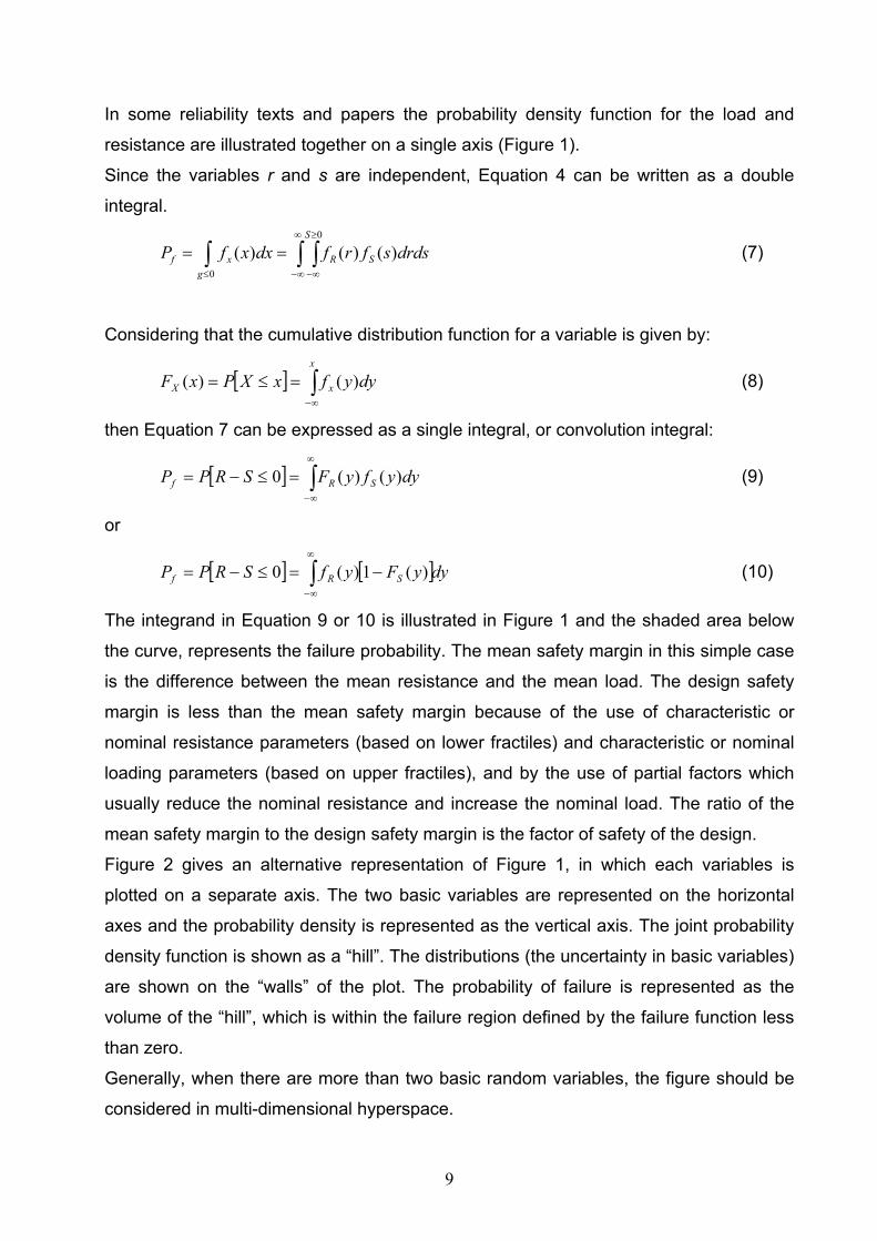
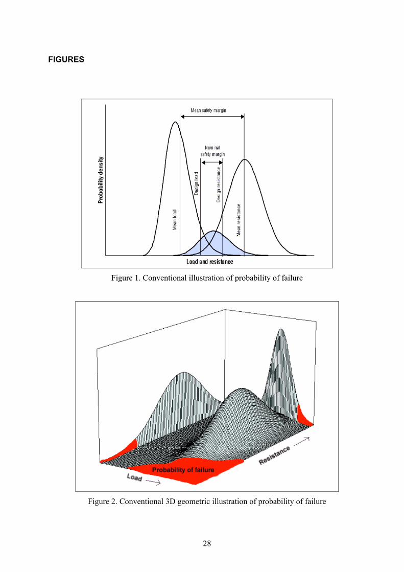
In some reliability texts and papers the probability density function for the load and

resistance are illustrated together on a single axis (Figure 1).

Since the variables r and s are independent, Equation 4 can be written as a double

integral.

(7) ∫ ∫ ∫≤

∞

∞−

≥

∞−

==0

0

)()()(g

S

SRxf drdssfrfdxxfP

Considering that the cumulative distribution function for a variable is given by:

(8) [ ] ∫∞−

=≤=x

xX dyyfxXPxF )()(

then Equation 7 can be expressed as a single integral, or convolution integral:

(9) [ ] ∫∞

∞−

=≤−= dyyfyFSRPP SRf )()(0

or

(10) [ ] [ dyyFyfSRPP SRf ∫∞

∞−

−=≤−= )(1)(0 ]

The integrand in Equation 9 or 10 is illustrated in Figure 1 and the shaded area below

the curve, represents the failure probability. The mean safety margin in this simple case

is the difference between the mean resistance and the mean load. The design safety

margin is less than the mean safety margin because of the use of characteristic or

nominal resistance parameters (based on lower fractiles) and characteristic or nominal

loading parameters (based on upper fractiles), and by the use of partial factors which

usually reduce the nominal resistance and increase the nominal load. The ratio of the

mean safety margin to the design safety margin is the factor of safety of the design.

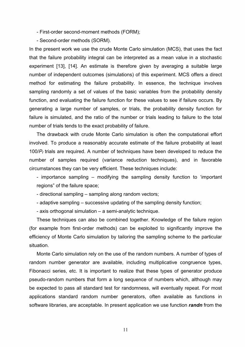
Figure 2 gives an alternative representation of Figure 1, in which each variables is

plotted on a separate axis. The two basic variables are represented on the horizontal

axes and the probability density is represented as the vertical axis. The joint probability

density function is shown as a “hill”. The distributions (the uncertainty in basic variables)

are shown on the “walls” of the plot. The probability of failure is represented as the

volume of the “hill”, which is within the failure region defined by the failure function less

than zero.

Generally, when there are more than two basic random variables, the figure should be

considered in multi-dimensional hyperspace.

9

3. PROBABILITY ANALYSIS

As already was mentioned the structural reliability and failure probability should always

be defined for a specified reference period of time. There are two classes of time

dependent problems which are generally considered:

- overload failure;

- cumulative failure.

The analysis of overload failure can be greatly simplified if time-varying resistance

effects (i.e. fatigue and corrosion) are being ignored. In this case the failure of structure

or structural component is going to occur under the maximum load effect during the

reference period or period of exposure. By treating the loading in this way the analysis

is termed time invariant reliability analysis.

In the case of cumulative failure, i.e. due to fatigue, corrosion, etc. , the total history of

the load up to the point in question is of importance. Failure may occur solely as the

results of cumulative loading, e.g. the formatting of a through-thickness crack due to

cyclic failure.

The structural reliability analysis for various failure modes requires an accurate model to

predict the failure. In present application the failure model is derived from the existing

deterministic model for crack growth rate (Paris law), and thermal fatigue damage due

to sin-wave temperature loading and non-uniform stress gradient through wall-thickness

[6].

As already discussed above, the probability of failure is defined:

[ ] ∫≤

=≤=0

)(0g

xf dxxfgPP (4’)

In some cases this equation can be integrated analytically. In principle, the

probability of failure or reliability can be evaluated using numerical integration

(trapezoidal rule, Simpson’s rule, etc.). In practice, this is not generally practical in

structural reliability because of the number of dimensions of the problem – one

dimension for each basic variable –, and because the area of interest is generally

located in the tails of the distributions. There are a number of other more commonly

used methods available for estimating the failure probability, and four are more often

used:

- Monte Carlo simulation methods;

- Mean value estimates;

10

- First-order second-moment methods (FORM);

- Second-order methods (SORM).

In the present work we use the crude Monte Carlo simulation (MCS), that uses the fact

that the failure probability integral can be interpreted as a mean value in a stochastic

experiment [13], [14]. An estimate is therefore given by averaging a suitable large

number of independent outcomes (simulations) of this experiment. MCS offers a direct

method for estimating the failure probability. In essence, the technique involves

sampling randomly a set of values of the basic variables from the probability density

function, and evaluating the failure function for these values to see if failure occurs. By

generating a large number of samples, or trials, the probability density function for

failure is simulated, and the ratio of the number or trials leading to failure to the total

number of trials tends to the exact probability of failure.

The drawback with crude Monte Carlo simulation is often the computational effort

involved. To produce a reasonably accurate estimate of the failure probability at least

100/Pf trials are required. A number of techniques have been developed to reduce the

number of samples required (variance reduction techniques), and in favorable

circumstances they can be very efficient. These techniques include:

- importance sampling – modifying the sampling density function to ‘important

regions” of the failure space;

- directional sampling – sampling along random vectors;

- adaptive sampling – successive updating of the sampling density function;

- axis orthogonal simulation – a semi-analytic technique.

These techniques can also be combined together. Knowledge of the failure region

(for example from first-order methods) can be exploited to significantly improve the

efficiency of Monte Carlo simulation by tailoring the sampling scheme to the particular

situation.

Monte Carlo simulation rely on the use of the random numbers. A number of types of

random number generator are available, including multiplicative congruence types,

Fibonacci series, etc. It is important to realize that these types of generator produce

pseudo-random numbers that form a long sequence of numbers which, although may

be expected to pass all standard test for randomness, will eventually repeat. For most

applications standard random number generators, often available as functions in

software libraries, are acceptable. In present application we use function randn from the

11

library of MATLAB Statistics Toolbox (which generates numbers from normal standard

distribution).

The Monte Carlo methods are an easily applied tool. They can be used to produce

‘exact” answers to problems, and can be used to provide answers to problems that

cannot be accurately modelled using first - or second-order methods. Such problems

include load combinations problems and time-varying problems (as fatigue).

4. PROSPECTIVE STUDY FOR PROBABILISTIC ANALYSIS APPLIED TO CIVAUX 1 CASE

In the following sections an example of the application of probability analysis on a case

study - Civaux 1 thermal fatigue damage – is illustrated. A description of the Civaux I

thermal fatigue damage case is given in the reference [15] and a short summary is

given below.

4.1 Case description In 1998 a longitudinal crack was discovered at outer edge of an elbow in a mixing zone

of the Residual Heat Removal System (RHRS) of the Civaux NPP unit 1. It is worth

mentioning that the time for crack development to a significant depth through the wall

was only about ≈1500 hours. The system operated at a pressure of 36 bar, the hot leg

contains water at 180o C and the cold leg contains water at 20oC. In the damage zone

of interest the pipe inner radius was ri ≅120 mm and outer radius was ro =129 mm.

Thermal and mechanical properties of austenitic steel (304L) at room temperature were

referred as: specific heat coefficient cheat=480 J/kg⋅C; thermal conductivity λ=14.7

W/m⋅C; mass density ρ=7800 kg/m3; mean thermal expansion α=16.4⋅10-6 C-1; Young’s

modulus E=177⋅109 Pa; Poison’s coefficient ν=0.3; thermal diffusivity coefficient

κ=3.93⋅10-6 m2/s.

The temperature fluctuation was reported to be in the range 20-180o C, and at the inner

surface of the pipe the maximum temperature fluctuation range was estimated to be

120oC. In the scope of the present work we consider a simple model for pipe as a

hollow cylinder having geometrical and material characteristics similar to those

mentioned before for Civaux 1 case. The transient temperature loading is considered in

the sin-wave form time dependence, which acts at inner surface of the cylinder, of

amplitude θ0=60 °C.

A deterministic study based on SIN-method has been developed [4], [6] and analytical

solutions for thermal and associated thermal stress were used to assess the crack

12

initiation and crack growth in a hollow cylinder. The main parameters in deterministic

analysis, which we also use in the probabilistic approach, are: pipe geometry, thermal

loading, critical frequencies, Paris law.

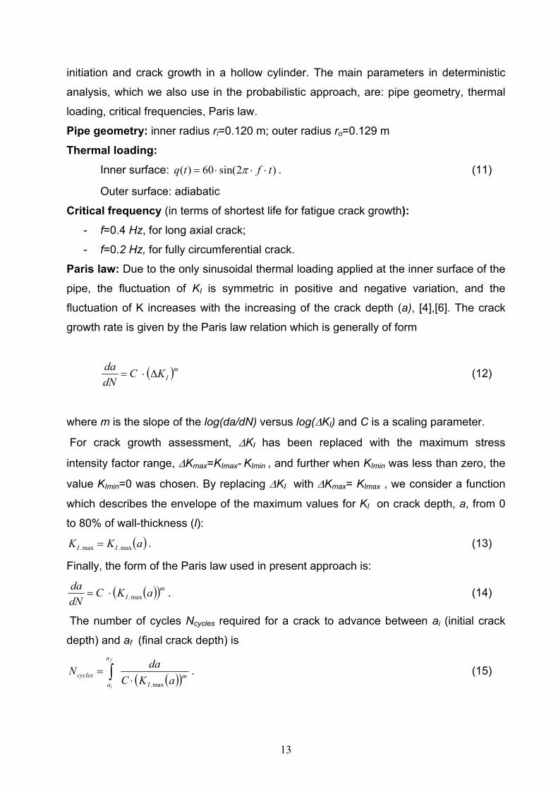
Pipe geometry: inner radius ri=0.120 m; outer radius ro=0.129 m

Thermal loading: Inner surface: )2sin(60)( tftq ⋅⋅⋅= π . (11)

Outer surface: adiabatic

Critical frequency (in terms of shortest life for fatigue crack growth): - f=0.4 Hz, for long axial crack;

- f=0.2 Hz, for fully circumferential crack.

Paris law: Due to the only sinusoidal thermal loading applied at the inner surface of the

pipe, the fluctuation of KI is symmetric in positive and negative variation, and the

fluctuation of K increases with the increasing of the crack depth (a), [4],[6]. The crack

growth rate is given by the Paris law relation which is generally of form

( )mIKC

dNda

∆⋅= (12)

where m is the slope of the log(da/dN) versus log(∆KI) and C is a scaling parameter.

For crack growth assessment, ∆KI has been replaced with the maximum stress

intensity factor range, ∆Kmax=KImax- KImin , and further when KImin was less than zero, the

value KImin=0 was chosen. By replacing ∆KI with ∆Kmax= KImax , we consider a function

which describes the envelope of the maximum values for KI on crack depth, a, from 0

to 80% of wall-thickness (l):

( )aKK II max.max. = . (13)

Finally, the form of the Paris law used in present approach is:

( )( mI aKC

dNda

max.⋅= )

)

. (14)

The number of cycles Ncycles required for a crack to advance between ai (initial crack

depth) and af (final crack depth) is

( )( mI

a

acycles aKC

daNf

i max.⋅= ∫ . (15)

13

The fatigue crack growth rates are in the units of mm/cycle with KI in units of MPa√m.

The threshold stress intensity factor range for this steel was assumed to be ∆Kth =5.0

MPa√m.

In previous works [4],[6], the ( )aKI max. dependence for two types of cracks have

been determined as follow:

a) long axial crack at the inner surface of the cylinder under hoop thermal stress

(f=0.4 Hz)

( ) 73.91071.31007.11017.5 22537max. +⋅⋅+⋅⋅−⋅⋅= aaaaKI (16)

b) fully circumferential crack at the inner surface of the cylinder under axial thermal

stress (f=0.2 Hz, fixed end boundary for the cylinder)

( ) 35.81068.31043.41022.3 32537max. +⋅⋅+⋅⋅−⋅⋅= aaaaKI . (17)

The information provided above are used in each Monte Carlo trial, in a manner which

are specified in the following sections.

4.2 Failure mode and function The present work on probabilistic approach of thermal fatigue crack growth depends on

the following basic elements:

- establishment of the limit states to be considered;

- identification of the failure modes that could lead to the limit states;

- construction of the limit state functions;

- data analysis and the construction of appropriate probability density functions;

- evaluation of failure probabilities;

The damage due to thermal fatigue in mixing tees is characterized by a high gradient of

thermal stress through the wall-thickness and as a consequence "long" shallow cracks

will appear at the pipe inner surface. During a thermal loading at the inner surface,

some of these cracks could penetrate the wall-thickness during the thermal loading, or

also can arrest. Leakage occurs with through-wall crack formation, most probable after

coalescence of long cracks. Therefore, a possibility is to perform fatigue crack

assessment considering a single equivalent crack with large crack shape ratio [8]. In the

present work we consider two type of cracks: long axial crack and fully circumferential

crack at the inner surface of the pipe.

This probabilistic approach considers as limit state of thermal fatigue damage due to

sinusoidal thermal loading a crack penetration depth of 80% wall thickness. Thus, it is

14

possible to define the failure function or limit state function as function of number of

thermal fatigue cycles, Ncycles, as

( ) ( )cyclesfcrcycles NaaNg −= (18)

or equivalent

cr

cyclesfcycles a

NaNg

)(1)( −= (19)

where acr is a critical depth of the fatigue crack, corresponding to 80% of the wall-

thickness, and af(Ncycles) is the final crack depth after N cycles of thermal loading. The

failure is predicted when the number of cycles Ncycles, will produce the following

condition

0)( ≤cyclesNg (20)

which means af > acr., failure condition. We should note that in the present study, we

consider long cracks; as a consequence the limit state function is referred just to the

crack depth.

During the Monte Carlo simulation (MCS), the trials which satisfy condition (20) are

accounted as nfail and the probability of failure for a certain period of time is given by

trials

failf N

nP = (21)

where Ntrials is the total number of trials simulation.

The limit state function, defined in Equations 18 or 19 contains the final crack depth,

af(Ncycles), which is obtained using the Paris law crack growth rate, in connection with a

specified period of time (Time). To specify that N cycle, time is fixed in this analysis.

The number of fatigue cycles (Ncycles) required to reach the final crack depth, af(Ncycles),

depends also on the loading frequency (f), as :

fTimeNcycles ×= . (22)

The frequency is fixed in this case by the sinusoidal load applied with 0.4Hz and

0.2Hz respectively.

The crack growth could be calculated on a cycle-by-cycle basis or as a group of N’

identical cycles. The crack size after the block of N’ cycles is given by

( )[ ]mbeforeIbeforeafter aKCNaa )(' max.⋅⋅+= . (23)

15

N’ is also referred to as the “blocking factor”, and the case of cycle-by-cycle crack

growth corresponding to N’=1 is used in the present work. As already mentioned the

crack length has not been considered, because just long axial crack and fully

circumferential crack (equations 16 and 17) are considered in the present prospective

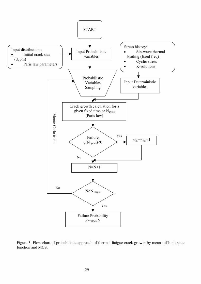
study. Figure 3 shows a flow chart of probabilistic approach used in the present study

based on crude MCS and limit state function from Equation (19).

The probabilistic variables used in this study were: the starting crack depth, ai, the Paris

law parameter C for a fixed m, while the deterministic variables were the thermal load at

the inner surface given a certain loading frequency, the correlated stress distributions

across the wall thickness, the K solutions for varying crack depth and a fixed number of

cycle or life time for evaluating the failure criteria.

4.3 Input parameters and distributions The distributions used in the paper to model parameters involved in thermal fatigue

crack growth are given in Appendix, see also [16].

During the Monte Carlo simulation it is necessary to model non-standard distributions in

a standard manner via a transformation and involving a standard normal distribution in

the following way as in Ref. [17].

Considering the cumulative form F(x) of the distribution concerned in the following

identity:

, (24) )()( uxF Φ=

where x is the variable concerned (i.e. initial crack depth ai or scaling parameter C from

Paris law), and Φ(u) is CDF (cumulative distribution function) for standard normal

distribution. The inverse of this is found:

. (25) ))((1 uFx Φ= −

and u is standard normally distributed variable [18] or uniform random number [19]. This

has the effect of forcing the variable x to adopt the required probability density function.

Crack size distribution The initial crack size distribution has a very strong influence on the deterministic and

also probabilistic assessment of a component lifetime. Usually, the initial crack

distribution involves three kinds of distributions:

- crack depth distribution;

- crack aspect ratio distribution;

16

- crack existence frequencies.

The present approach considers only cracks that start out as long inner surface cracks,

characterized by initial crack depth distribution as an exponential distribution [20]. The

corresponding probability density function (pdf) is

( ) µ

µµ

x

exf−

=1; , x≥0; µ>0 (26)

In present work we adopted the pdf from equation (26) in the following form

( ) a

a

aa eap µ

µµ

−

=1; 00 aa ≤≤ (27)

For a pipe thickness l=9 mm as in the present work, we consider a mean value of the

crack depth as

µa=1 mm (28)

and the coefficient of variation in this case is CoV=1. The mean value of the crack depth

is small, but in deterministic assessments this value is generally assumed as a started

depth for fatigue crack growth. The proposed value to be used for a0 in Eq.(27), which

usually is considered ∞ in the case of thick pipe-wall, can be seen as cracks detected

by ISI, before assessment. Therefore, in this application, a value of 3 mm is chosen,

which means about 30% of the wall pipe. In this way the cracks with depth bigger than 3

mm, generated by MC sampling from exponential distribution, are not accounted for

crack growing.

The exponential distribution is used to produce random value for initial crack depth ai,

with the following sequence in MATLAB Statistics Toolbox [21]:

ai= ;µ( auF µ);(1 Φ− )

)

a=1mm; (29)

where is the MATLAB inverse function of exponential cumulative

distribution function (CDF) and Φ(u) is CDF for standard normal distribution.

( auF µ);(1 Φ−

Paris law parameters distribution For this study, the fatigue crack growth rates were calculated using stainless steel crack

growth law given in ASME [22]:

( )mIKC

dNda

∆⋅= (30)

17

where m=3.3 is the slope of the log(da/dN) versus log(∆KI) and C is a scaling

parameter. Slopes (m) and intercepts (C) for all fatigue data are usually highly

correlated. Ignoring this correlation can give misleading results in a simulation.

An alternate method to account for this correlation is to use a constant slope and put all

of variability into the intercept. For a constant slope, the variability in fatigue lives will be

directly related to variability in the material constant C. The scatter in the experimental

fatigue data is represented by a lognormal distribution for C scaling parameter, with the

following pdf

( )2

0

0ln21

000 2

1,;

−−

⋅= σ

µ

πσσµ

x

ex

xf , (31)

where µ0, σ0, are parameters, calculated from the median/mean value and standard

deviation as shown in Appendix.

From reference [8] we consider the following parameters:

Median: Cmedian=10.04⋅10-12 (m/cycle/ MPa√m) , (32)

Standard deviation: σC=2.2⋅10-11 . (33)

With these parameters a mean value is derived as Cmean= 1.664⋅10-11 and coefficient of

variation by CoV=1.32. The log-normal distribution is used to produce random values

for C constant in Paris law with the following sequence in MATLAB Statistics Toolbox:

C= ; µ( 001 ,);( σµuF Φ− )

)

0= - 25.3244; σ0=1.0053. (34)

Here is the MATLAB function for inverse function of log-normal CDF.

The parameters µ

( 001 ,);( σµuF Φ−

0 and σ0 were derived with relationships from Appendix.

4.4 Analysis and discussion The probabilistic approach of thermal fatigue crack growth by means of crude Monte

Carlo simulation and based on the limit state function (failure function) follows the main

steps from flow chart shown in Figure 3. To develop a prospective study for probabilistic

fatigue approach, the Civaux 1 fatigue damage case is used, where a crack growth

fatigue life of 1000 hours was estimated [6].

Procedure is summarized below.

Geometry:

• a pipe model with main parameters from Civaux 1 fatigue damage case and

thermal loading as sin-wave time dependence with fixed frequency at the inner

pipe surface is assumed;

18

Defects:

• long shallow defects exist at the inner surface of the pipe (axial or

circumferential), and after growing through the wall-thickness they are not

coalesced with the other;

• the defects originated at the inner surface grow only due to the thermal stresses

arising from sinusoidal thermal loading applied at the inner surface;

• it is assumed that the initial crack depth distribution follows the exponential

distribution; none crack shape distributions are considered;

Crack growth:

• the crack growth rate is given by Paris law, and dependence on crack depth,

∆Kmax= KImax(a), have been obtained for long axial and circumferential cracks

under associated elastic thermal stresses in previous works;

• the scatter in the experimental fatigue data is represented by a lognormal

distribution for value of scaling parameter C; the slope m has a specified fixed

value;

Method:

• the crude Monte Carlo method is used in simulation (see flow chart in Figure 3);

• the procedure uses the limit state function approach to obtain probability of

failure, Pf, for a specified fixed period of time (or for a defined fatigue life);

• the empirical cumulative density function approach is used to benchmark results

for Pf.

The specific routines were implemented to perform the trials in concordance with the

sequences from the flaw chart shown in Figure 3, using Statistics Toolbox from

MATLAB software.

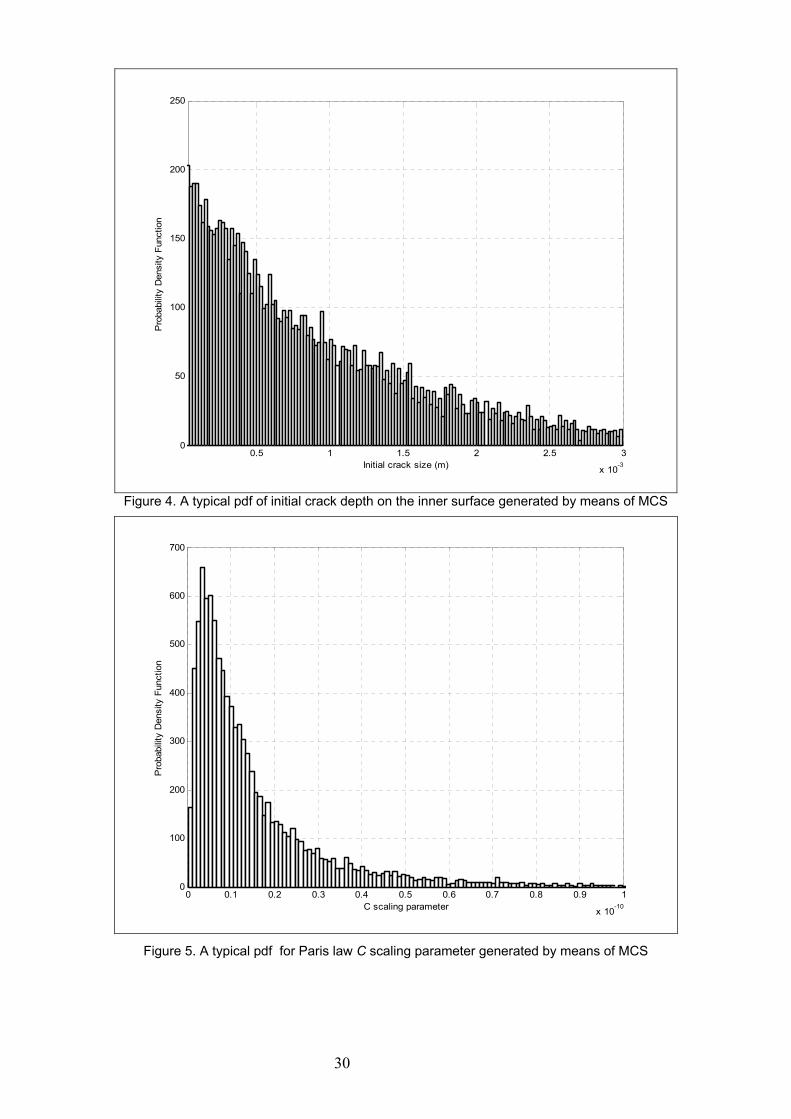
For a MC sampling simulation of 104-105 trials, a typical pdf histogram for initial crack

depth distribution is shown in Figure 4, which is based on the hypotheses of a mean

value of the crack µa= 1mm, and that flaws grater then 3 mm don’t exist. Note that these

hypotheses are not based on the real ISI measurements, but they are useful for a

prospective analysis. As can be seen, it approximates quite well the shape of known

theoretical exponential pdf. In the case of Paris law C scaling parameter the log-normal

pdf histogram is shown in Figure 5, with modeling parameters already mentioned.

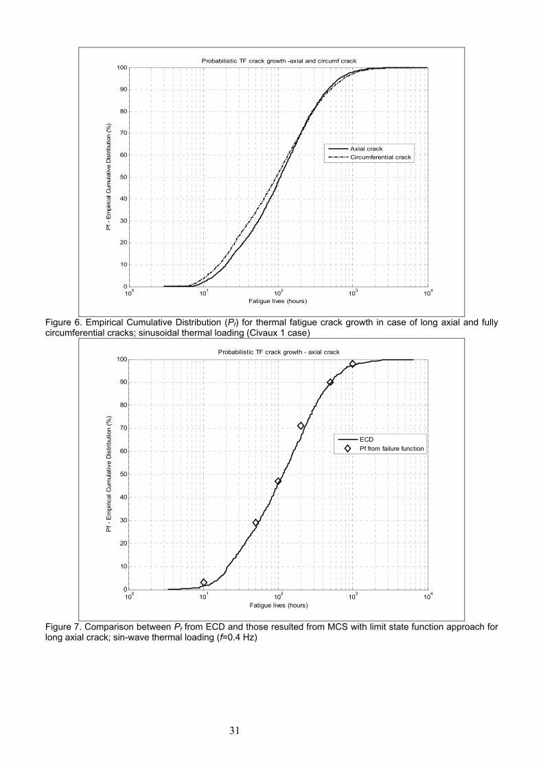
The result of MC simulations gives the probabilities associated with crack growth lives

for specified periods of time (fatigue lives), for both axial and circumferential crack. In

19

order to check the probabilities failure predictions obtained by means of limit state

function, we use the empirical cumulative distribution (ECD) (see Appendix) to

represent an output from the Monte Carlo simulation in sense of cumulative probability

of failure, Pf. Thus, it is firstly derived Pf and Figure 6 compares these ECDs for axial

and circumferential crack as function of fatigue lives in hours. Dependences have

typical shape for both directions and slightly higher Pf predictions are obtained for

circumferential crack up to fatigue lives of 200 hours.

In the case of probabilistic fatigue assessment for axial crack by means of failure

function and MCS, the sinusoidal thermal loading with frequency f=0.4 Hz has been

considered. We have to recall that this frequency was found to be the critical frequency

in term of shortest life for long axial crack [6]. By using Paris law within MCS trials with

dependence from equation (16) and failure function g(N( )aKI max. cycles) given by

equation (19) the results are plotted in Figure 7. A good agreement is found with

predictions from ECD for whole range of fatigue lives.

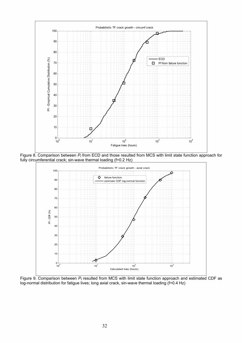
In the case of probabilistic fatigue assessment for circumferential crack, a similar

estimation as before, but with f=0.2 Hz and ( )aKI max. dependence from equation (17),

has been done. The comparison with predictions from ECD is shown in Figure 8.

Figures 7 and 8 show that the crack growth lifetime of 1000 hours has a very high

probability to occur, although only thermal stresses have been used in the assessment.

An important task is to estimate cumulative distribution functions for fatigue lives after

finding probabilities failure associated with corresponding fatigue lives. The following

characteristics of fatigue life distributions were estimated, by means of the specific

MATLAB functions from Statistics Toolbox: probability density function, associated

mean value of life and coefficient of variation (CoV). The log-normal distribution has

been found to best fit the results from failure function approach with MCS, for both

cases. The results of fitting are summarized in the next.

Long axial crack growth (f=0.4 Hz):

- pdf: ( )2

0

0ln21

000 2

1,;

−−

⋅= σ

µ

πσσµ

x

ex

xf ; µ0=4.63; σ0=1.20; (35)

- mean=212 hours;

- CoV=1.83.

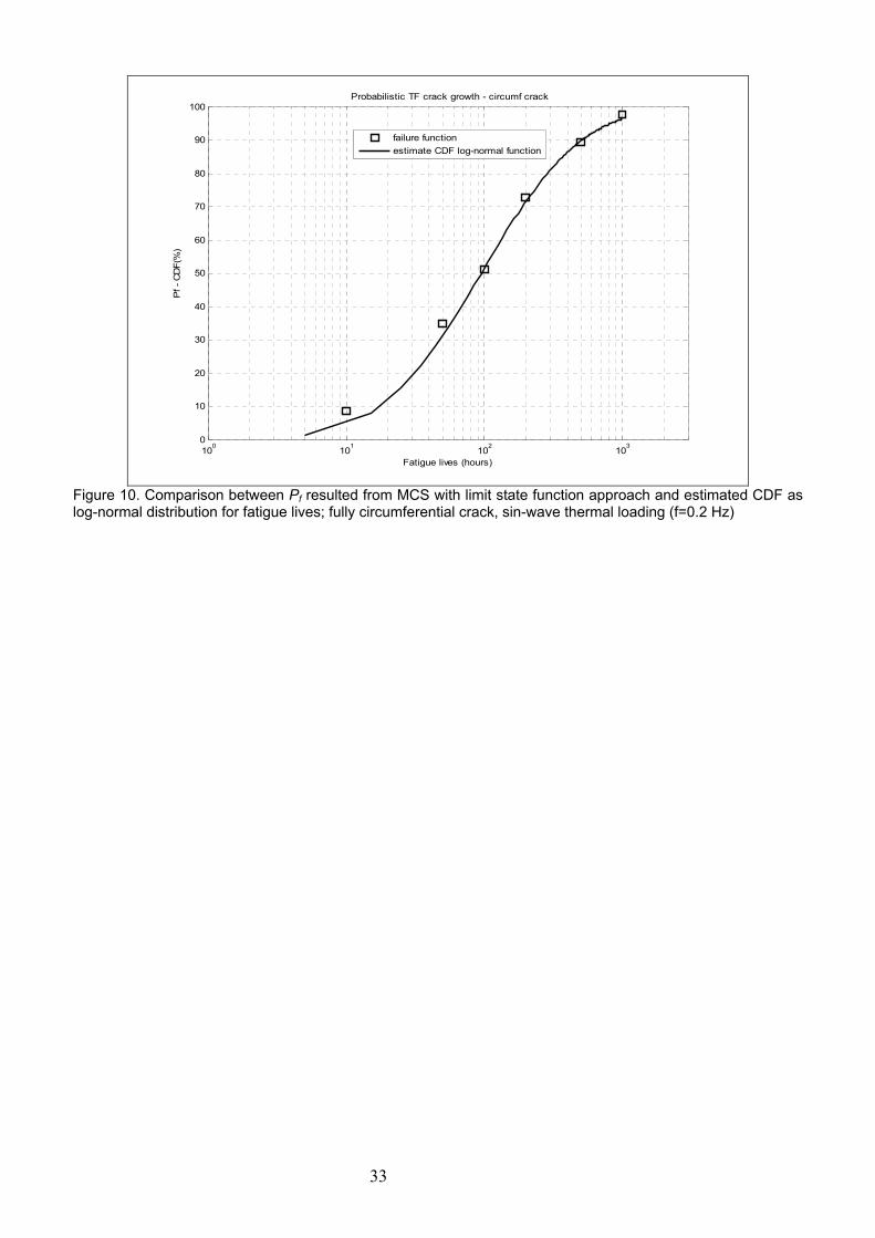
Fully circumferential crack growth (f=0.2 Hz):

20

- pdf: ( )2

0

0ln21

000 2

1,;

−−

⋅= σ

µ

πσσµ

x

ex

xf ; µ0=4.52; σ0=1.30; (36)

- mean=223 hours;

- CoV=2.13.

Figures 9 and 10 show a comparison between cumulative distribution functions

estimated with parameters from Equations (35) and (36), and results from approach of

limit state function. The agreement is quite good for both cases and we can conclude

that fatigue lives in this case of fatigue crack growth follow a log-normal distribution.

However, the parameters which define the mentioned pdf (Equations 35 and 36) were

derived assuming some hypothesis (initial mean value of the initial crack depth, a

constant slope m, sin-wave thermal loading, only thermal stresses, etc.). More refined

probabilistic analysis needs to be performed in order to account for a realistic thermal

loading spectrum, and also the variability of more specific parameters.

5. CONCLUSIONS

The present work performs a prospective study on probabilistic approach of thermal

fatigue in mixing tees (Civaux 1 damage case) by means of the limit state function and

Monte Carlo simulation. It is based on previous work where a deterministic assessment

for thermal fatigue crack growth in high-cycle loadings, under the large nonlinear

gradient stress profiles through wall-thickness due to sinusoidal thermal loading, has

been done.

The probabilistic approach considers variability in initial crack depth and Paris law C

scaling parameter by means of specific probability density distributions. A given

sinusoidal load has been considered as first step approach, even though the real load

represents the main variable, being the most difficult to be determined. In the case of

first variable a hypothetic mean value of initial crack depth is adopted, and for second

one values from literature are used. The crude Monte Carlo Simulations are performed

using specific routines implemented in MATLAB software with Statistics Toolbox, and

probabilities of failure are derived using the failure function which is defined based on a

21

limit state given by the critical crack depth. The results were checked against

predictions from empirical cumulative distribution and good agreements was found. An

important task was to estimate distribution function for fatigue lives after finding

probabilities failure associated with corresponding fatigue lives by means of the failure

function approach. Using specific MATLAB functions from Statistics Toolbox, for both

axial and circumferential cracks, then the pdf, associated mean value of the fatigue life

and CoV have been estimated. The log-normal distribution has been found to best fit

the results from failure function approach with MCS, for both cases.

The prospective study results will be used for a probabilistic approach of thermal fatigue

in mixing tees (initiation and crack growth), based on a realistic thermal loading

spectrum and mechanical loading, and also for the variability of more specific

parameters.

22

GLOSSARY

Basic variables: A set of variables entering the failure function equation to define failure.

They may include basic engineering parameters, such as wall thickness,

yield stress, allowed crack depth etc., as well as model uncertainty in the

failure function itself.

Beta-point: The point with maximum probability density, and values of the basic

variables at this point represent the most probable values to cause

failure.

CoV (Coefficient of Variation): The ratio of standard deviation to mean value of a

variable:

X

CoVµσ

= .

Expected value, E[X ]): The mean value of a variable. It is defined as first moment of the

distribution function of a variable, and is evaluated from distribution

function fX(x):

. [ ] ∫∞

∞−

== dxxfXE XX )(µ

Failure function, g: The failure function (or limit state function) in reliability analysis is a

mathematical function used to predict the failure event for a component,

part of a structure, or a structural system. The failure function is

expressed in terms of basic variables, and is defined such that g≤0

correspond to failure.

Model uncertainty: The inherent uncertainty associated with the mathematical models

used to predict resistance (and loading).

Probability of failure, Pf: The probability of failure of an event is the probability that

the limit state criterion or failure function defining the event will be

exceeded in a specified reference period.

Probability density function, pdf: The probability that a random variable X shall appear

in the interval [x, x+dx] is fX(x)dx where fX(x) is the probability density.

Reference period: Reliabilities and probabilities of failure should be defined in terms of

a reference period, which may typically be one year of the design life.

Reliability: The probability that a component will fulfill its design purposes. Defined

as 1-Pf.

23

Reliability index,β: A useful measure to compare Pfs. it is defined using the standard

normal distribution function Φ(u),

( ) ( )ff PP 11 1 −− Φ−=−Φ=β .

Standard deviation, Sd[X ] or σ: The standard deviation is defined as square root of

the Variance of a variable:

)(XVar=σ

Standard normal space, U-space: A space of independent normally distributed random

variable with zero mean and unit standard deviation. Basic variable

space is transformed into standard normal space in some reliability

analysis procedures (FORM, SORM).

Variance, Var[X ]: The variance of a variable is defined as the second central moment

of the distribution function of a variable, and is evaluated from the

distribution function fX(x):

, [ ] ( )∫∞

∞−

−= dxxfxxXVar XX )()( 2µ

where µX is the mean or expected value.

24

APPENDIX: THE CDFS AND PDFS USED FOR PROBABILISTIC FATIGUE APPROACH

a) Normal distribution (Gauss distribution) Probability density function (pdf):

( )2

21

21,;

−

−= σ

µ

πσσµ

x

exf , -∞<x<∞; -∞<µ<∞; σ2>0. (A1)

Cumulative distribution function (CDF):

( ) ( ) dttxFx

∫∞−

−−= 2

2

2exp

21,;

σµ

πσσµ (A2)

Note: For µ=0 and σ=1 we refer to this distribution as standard normal distribution

( )2

21

21 x

exf−

=π

(A3)

which has the cumulative distribution (CFD)

dttuu

∫∞−

−=Φ

2exp

21)(

2

π (A4)

Moments:

mean (expected value):

( ) µµ == XXE . (A5)

variance:

(A6) ( ) 2σ=XVar

standard deviation:

( )XVar=σ (A7)

b) Exponential distribution Probability density function (pdf):

( ) µ

µµ

x

exf−

=1; x≥0; µ>0 (A8)

Cumulative distribution function (CDF):

( ) µµx

exF−

−= 1; . (A9)

Moments:

mean (expected value):

25

( ) µµ == XXE . (A10)

variance:

(A11) ( ) 2µ=XVar

standard deviation:

( ) µσ == XVar . (A12)

The exponential (Marshal) distribution is used to produce random value for initial crack

depth ai.

c) Log-normal distribution Probability density function (pdf):

( )2

0

0ln21

000 2

1,;

−−

⋅= σ

µ

πσσµ

x

ex

xf (A13)

Cumulative distribution function (CDF):

( ) ( ) dttt

xFx

∫

−−⋅=

020

20

000 2

)ln(exp12

1,;σ

µπσ

σµ (A14)

with µ0, σ0, parameters.

Moments:

mean (expected value):

( ) 2

20

0σ

µµ

+== eXE X (A15)

variance:

( ) ( )120

2002 −= + σσµ eeXVar (A16)

standard deviation:

( )XVar=σ (A17)

median:

(A18) 0µemed =

The log-normal distribution is used to produce random value for C constant in Paris law

and to fit fatigue lives distribution.

d) Empirical cumulative distribution The cumulative distribution function is given by

(A19) ( ) ∫∞−

=x

dttfxF )(

for a continuum variable and by

26

(A20) ∑≤

=xy

ii

yfxF )()(

for a discrete random variable.

When is not suitable to assume a distribution for a random variable, then we can use a

cumulative distribution function called the empirical distribution function, as an estimate

of the underlying distribution. One can call this a nonparametric estimate of a

distribution function, because it is not assuming a specific parametric form for the

distribution that generates the random phenomena. In a parametric setting we would

assume a particular distribution generated the sample and estimate the cumulative

distribution function by estimating the appropriate parameters.

The empirical distribution function is based on the order statistics. The order statistics

for a sample are obtained by putting the data in ascending order. Thus, for a random

sample of size n, the order statistics are defined as

, (A21) )()4()3()2()1( ... nXXXXX ≤≤≤≤

with X(i) denoting the ith order statistic. The empirical distribution function Fn(x) is defined

as the number of data points less than or equal to x (#(Xi≤x)) divided by the sample size

n. It can be expressed in terms of the order statistics as follows

≥

≤≤

<

= +

)(

)1()(

)1(

;1

;

;0

)(

n

jjn

Xx

XxXnj

Xx

xF (A22)

We use the empirical cumulative distribution (ECD) to represent an output from the

Monte Carlo simulation in sense of cumulative probability of failure for estimated fatigue

life derived by means of Paris law fatigue crack growth.

27

FIGURES

Figure 1. Conventional illustration of probability of failure

Figure 2. Conventional 3D geometric illustration of probability of failure

28

START

Input Probabilistic variables

Input distributions: • Initial crack size

(depth) • Paris law parameters

Monte C

arlo trials

No

No

Yes

Yes

Failure Probability Pf=nfail/N

N≥NTarget

N=N+1

nfail=nfail+1 Failure g(Ncycles)<0

Crack growth calculation for a given fixed time or Ncycle

(Paris law)

Probabilistic Variables Sampling

Stress history: • Sin-wave thermal

loading (fixed freq) • Cyclic stress • K-solutions

Input Deterministic variables

Figure 3. Flow chart of probabilistic approach of thermal fatigue crack growth by means of limit state function and MCS.

29

0.5 1 1.5 2 2.5 3

x 10-3

0

50

100

150

200

250

Initial crack size (m)

Pro

babi

lity

Den

sity

Fun

ctio

n

Figure 4. A typical pdf of initial crack depth on the inner surface generated by means of MCS

0 0.1 0.2 0.3 0.4 0.5 0.6 0.7 0.8 0.9 1

x 10-10

0

100

200

300

400

500

600

700

C scaling parameter

Pro

babi

lity

Den

sity

Fun

ctio

n

Figure 5. A typical pdf for Paris law C scaling parameter generated by means of MCS

30

100 101 102 103 1040

10

20

30

40

50

60

70

80

90

100

Fatigue lives (hours)

Pf -

Em

piric

al C

umul

ativ

e D

istri

butio

n (%

)

Probabilistic TF crack growth -axial and circumf crack

Axial crackCircumferential crack

Figure 6. Empirical Cumulative Distribution (Pf) for thermal fatigue crack growth in case of long axial and fully circumferential cracks; sinusoidal thermal loading (Civaux 1 case)

100

101

102

103

104

0

10

20

30

40

50

60

70

80

90

100

Fatigue lives (hours)

Pf -

Em

piric

al C

umul

ativ

e D

istri

butio

n (%

)

Probabilistic TF crack growth - axial crack

ECDPf from failure function

Figure 7. Comparison between Pf from ECD and those resulted from MCS with limit state function approach for long axial crack; sin-wave thermal loading (f=0.4 Hz)

31

100 101 102 103 1040

10

20

30

40

50

60

70

80

90

100

Fatigue lives (hours)

Pf -

Em

piric

al C

umul

ativ

e D

istri

butio

n (%

)

Probabilistic TF crack growth - circumf crack

ECDPf from failure function

Figure 8. Comparison between Pf from ECD and those resulted from MCS with limit state function approach for fully circumferential crack; sin-wave thermal loading (f=0.2 Hz)

100 101 102 1030

10

20

30

40

50

60

70

80

90

100

Calculated lives (hours)

Pf -

CD

F (%

)

Probabilistic TF crack growth - axial crack

failure functionestimate CDF log-normal function

Figure 9. Comparison between Pf resulted from MCS with limit state function approach and estimated CDF as log-normal distribution for fatigue lives; long axial crack, sin-wave thermal loading (f=0.4 Hz)

32

100 101 102 1030

10

20

30

40

50

60

70

80

90

100

Fatigue lives (hours)

Pf -

CD

F(%

)

Probabilistic TF crack growth - circumf crack

failure functionestimate CDF log-normal function

Figure 10. Comparison between Pf resulted from MCS with limit state function approach and estimated CDF as log-normal distribution for fatigue lives; fully circumferential crack, sin-wave thermal loading (f=0.2 Hz)

33

34

REFERENCES

[1] S. R. Gosselin, F. A. Simonen, S. P. Pili, B. O. Y. Lydell, Probabilities of Failure and Uncertainty estimate

Information for Passive Components – A literature review, NUREG/CR-6936, PNNL-16186, May 2007,

U.S. Nuclear Regulatory Commission, Washington, DC 20555-0001, NRC Job Code N6019.

[2] IAEA-TECDOC-1361, Assessment and management of ageing of major nuclear power plant components

important to safety-primary piping in PWRs, IAEA, July 2003.

[3] V. Radu, E. Paffumi, N. Taylor, New analytical stress formulae for arbitrary time dependent thermal loads

in pipes, European Commission Report EUR 22802 DG JRC, June 2007, Petten, NL.

[4] V. Radu, E. Paffumi, N. Taylor, K.-F. Nilsson, Assessment of thermal fatigue crack growth in the high

cycle domain under sinusoidal thermal loading – An application-Civaux 1 case, published as European

Commission Report EUR 23223 EN, ISSN: 1018-5593, ISBN: 978-92-79-08218-4, DOI: 10.2790/4943,

DG JRC, 2007, Petten, The Netherlands.

[5] V. Radu, N. Taylor, E. Paffumi, Development of new analytical solutions for elastic thermal stress

components in a hollow cylinder under sinusoidal transient thermal loading, International Journal of

Pressure Vessels and Piping 85 (2008) 885-893.

[6] V. Radu E. Paffumi N. Taylor K.-F. Nilsson, A study on fatigue crack growth in high cycle domain

assuming sinusoidal thermal loading, paper under revision in International Journal of Pressure Vessels

and Piping.

[7] M. A. Khaleel, F. A. Simonen, Effect of through-wall stress gradients on piping failure probabilities,

Nuclear Engineering and Design 197 (2000) 89-106

[8] S.R. Gosselin, F.A. Simonen, P.G. Heasler, S.R. Doctor, Fatigue Crack Flaw Tolerance in Nuclear Power

Plant Piping ; A basis for Improvements to ASME Code Section XI Appendix L, NUREG/CR-6934, PNNL-

16192, May 2007.

[9] I. Varfolomeyev, Probabilistic analysis of cracking phenomenon in a mixing tee under thermal fatigue,

Proceedings of PVP 2007, 2007 ASME Pressure Vessels and Piping Division Conference, July 22-26,

2007, San Antonio, Texas.

[10] Z. Guédé, B. Sudret, M. Lemaire, Life-time reliability based assessment of structures submitted to thermal

fatigue, International Journal of Fatigue 29 (2007) 1359-1373.

[11] B. Sudret, Z. Guédé, Probabilistic assessment of thermal fatigue in nuclear components, Nuclear

Engineering and Design 235 (2005) 1819-1835.

[12] James W. Provan (editor), Probabilistic fracture mechanics and reliability, 1987 by Martinus Nijhoff

Publishers, Dordrecht, The Netherlands.

[13] O. Ditlevsen and H. O. Madsen, Structural Reliability Methods, Monograph, John Wiley & Sons Ltd, CW,

2007

[14] W. J. Metzger, Statistical Methods in Data Analysis, Nijmegen, The Netherlands, June 2002

[15] S. Chapuliot, C. Gourdin, T. Payen, J.P. Magnaud, A. Monavon, Hydro-thermal-mechanical analysis of

thermal fatigue in a mixing tee, Nuclear Engineering and Design 235 (2005) 575-596.

[16] C. L. Atwood, J. L. LaChance, H. F. Martz, D. J. Anderson, M. Englehardt, D. Whitehead, T. Wheeler,

Handbook of Parameter Estimation for Probabilistic Risk Assessment, NUREG/CR-6823, SAND2003-

3348P, September 2003, U.S. Nuclear Regulatory Commission, Washington, DC 20555-0001, NRC Job

Code W6970

35

[17] Wendy L. Martinez, Angel R. Martinez, Computational Statistics Handbook with MATLAB, Chapman &

Hall/CRC 2002.

[18] B. Limited, Probabilistic methods: Uses and abuses in structural integrity, HSE books, 2001

[19] The MathWorks, Statistics Toolbox User’s Guide, version 5, 2005

[20] Peter Dillström, ProSINTAP – A probabilistic program implementing the SINTAP assessment

procedure, Engineering Fracture Mechanics 67 (2000) 647-668.

[21] The MathWorks, Statistics Toolbox For Use with MATLAB, User’s Guide, version 3, 2001.

[22] ASME, 2004 ASME Boiler & Pressure Vessel Code XI, Rules for In-service Inspection of Nuclear Power

Plant Components, New York, 2004 Edition July 1, 2004.

European Commission EUR 23570 EN – Joint Research Centre – Institute for Energy Title: A prospective study for probabilistic approach of thermal fatigue in mixing tees Author(s): V. Radu, E. Paffumi, N. Taylor, K. –F. Nilsson Luxembourg: Office for Official Publications of the European Communities 2009 – 35 pp. – 21 x 29.7 cm EUR – Scientific and Technical Research series – ISSN 1018-5593 Abstract The work performs a prospective study on probabilistic approach of thermal fatigue in mixing tees (Civaux 1 damage case) by means of the limit state function and Monte Carlo simulation. It is based on previous work where a deterministic assessment for thermal fatigue crack growth in high-cycle loadings, under the large nonlinear gradient stress profiles through wall-thickness due to sinusoidal thermal loading, has been done. The probabilistic approach considers variability in initial crack depth and Paris law C scaling parameter by means of specific probability density distributions. The crude Monte Carlo Simulations are performed using specific routines implemented in MATLAB software with Statistics Toolbox, and probabilities of failure are derived using the failure function which is defined based on a limit state given by the critical crack depth. The results were checked against predictions from empirical cumulative distribution and a good agreement was found. An important task was to estimate distribution function for fatigue lives after finding probabilities failure associated with corresponding fatigue lives by means of the failure function approach. Using specific MATLAB functions from Statistics Toolbox, the probability density function, associated mean value of the fatigue life and CoV have been estimated for both axial and circumferential crack growth. The log-normal distribution has been found to best fit the results from failure function approach with MCS, for both cases.

The mission of the JRC is to provide customer-driven scientific and technical support for the conception, development, implementation and monitoring of EU policies. As a service of the European Commission, the JRC functions as a reference centre of science and technology for the Union. Close to the policy-making process, it serves the common interest of the Member States, while being independent of special interests, whether private or national.