'
&
$
%
General Outline
• Part 0: Background, Motivation, and Goals.
• Part I: Some Basics.
• Part II: Diversity Systems.
• Part III: Co-Channel Interference.
• Part IV: Multi-Hop Communication Systems.
'
&
$
%
Outline - Part III: Co-Channel Interference
1. Co-Channel Interference (CCI) Analysis
• Effect of Shadowing
• Effect of Multipath Fading
– Single Interferer
– Multiple Interferers
– Minimum Desired Signal Requirement
– Random Number of Interferers
2. CCI Mitigation
• Diversity Combining
• Optimum Combining/Smart Antennas
• Optimized MIMO Systems in Presence of CCI
'
&
$
%
Effect of Shadowing
• Finding the statistics of the sum of log-normalrandom variables.
• No known exact closed-form available.
• Several analytical techniques have been devel-oped over the years.
• As an example, we cover the Farley bounds onthe sum of log-normal random variables.
'
&
$
%
Effect of Multipath Fading (1)
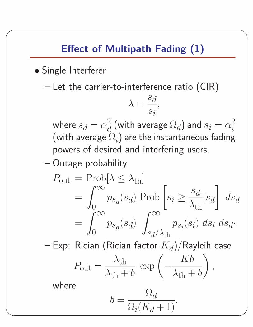
• Single Interferer
– Let the carrier-to-interference ratio (CIR)
λ =sd
si,
where sd = α2d (with average Ωd) and si = α2
i(with average Ωi) are the instantaneous fadingpowers of desired and interfering users.
– Outage probability
Pout = Prob[λ ≤ λth]
=
∫ ∞
0psd(sd) Prob
[si ≥
sd
λth|sd
]dsd
=
∫ ∞
0psd(sd)
∫ ∞
sd/λth
psi(si) dsi dsd·
– Exp: Rician (Rician factor Kd)/Rayleih case
Pout =λth
λth + bexp
(− Kb
λth + b
),
where
b =Ωd
Ωi(Kd + 1).
'
&
$
%
Effect of Multipath Fading (2)
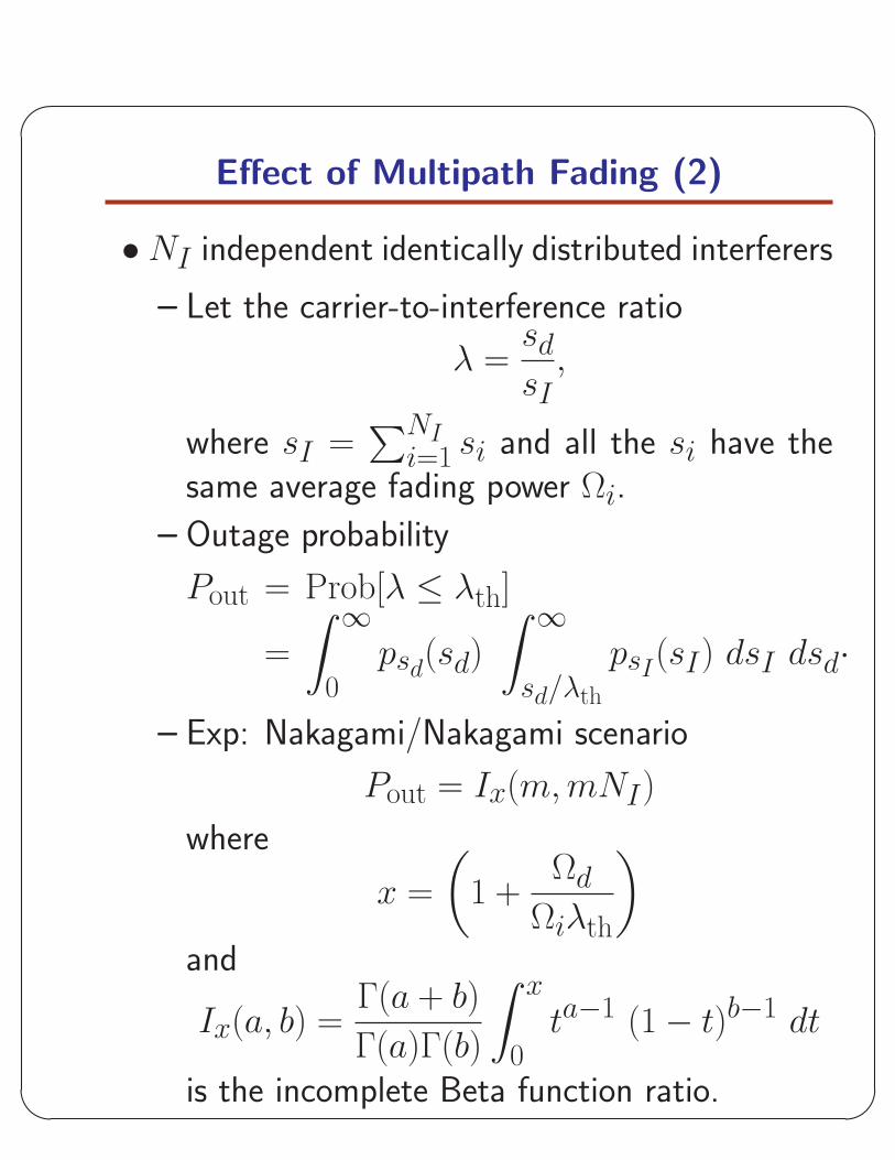
• NI independent identically distributed interferers
– Let the carrier-to-interference ratio
λ =sd
sI,
where sI =∑NI
i=1 si and all the si have thesame average fading power Ωi.
– Outage probability
Pout = Prob[λ ≤ λth]
=
∫ ∞
0psd(sd)
∫ ∞
sd/λth
psI(sI) dsI dsd·
– Exp: Nakagami/Nakagami scenario
Pout = Ix(m,mNI)
where
x =
(1 +
Ωd
Ωiλth
)
and
Ix(a, b) =Γ(a + b)
Γ(a)Γ(b)
∫ x
0ta−1 (1− t)b−1 dt
is the incomplete Beta function ratio.
'
&
$
%
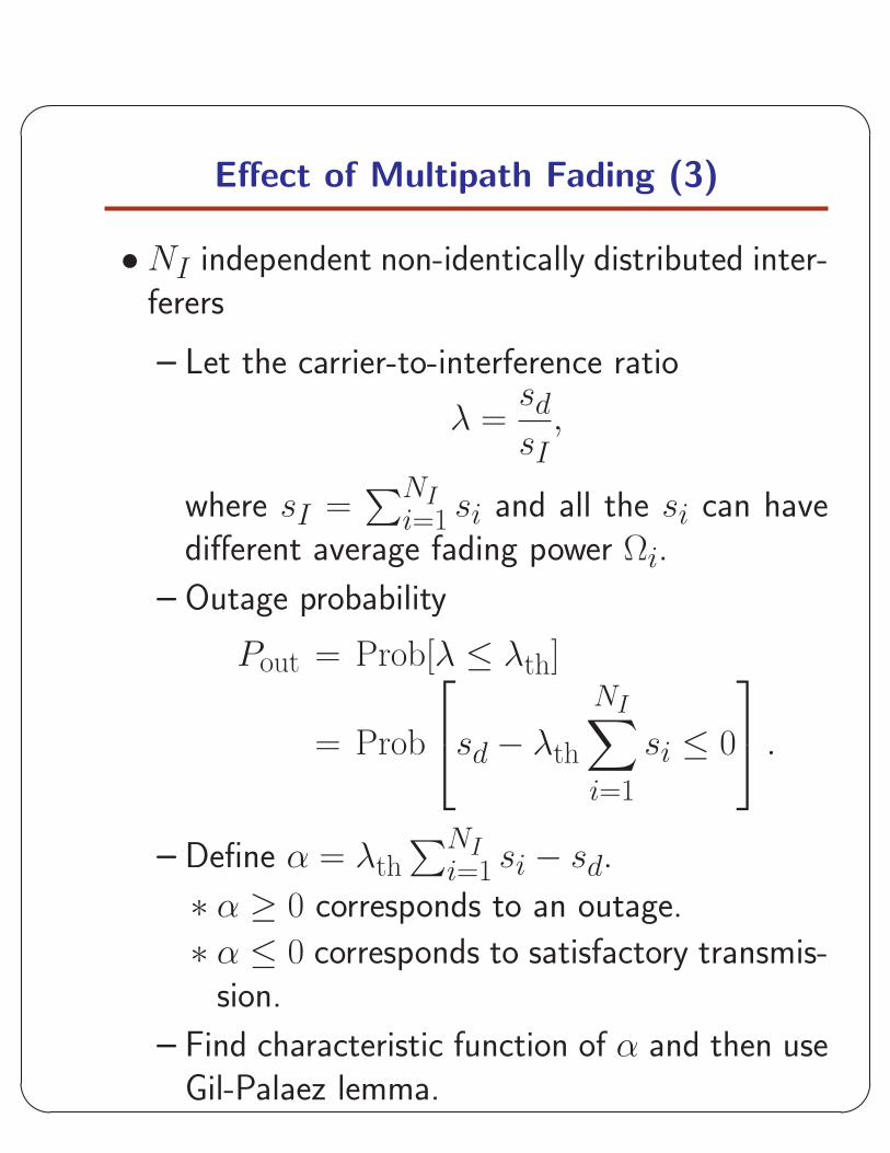
Effect of Multipath Fading (3)
• NI independent non-identically distributed inter-ferers
– Let the carrier-to-interference ratio
λ =sd
sI,
where sI =∑NI
i=1 si and all the si can havedifferent average fading power Ωi.
– Outage probability
Pout = Prob[λ ≤ λth]
= Prob
sd − λth
NI∑
i=1
si ≤ 0
.
– Define α = λth∑NI
i=1 si − sd.
∗ α ≥ 0 corresponds to an outage.
∗ α ≤ 0 corresponds to satisfactory transmis-sion.
– Find characteristic function of α and then useGil-Palaez lemma.
'
&
$
%
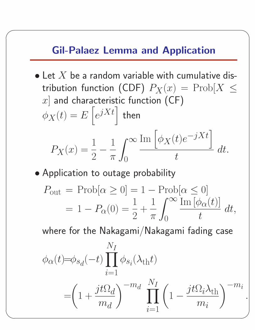
Gil-Palaez Lemma and Application
• Let X be a random variable with cumulative dis-tribution function (CDF) PX(x) = Prob[X ≤x] and characteristic function (CF)
φX(t) = E[ejXt
]then
PX(x) =1
2− 1
π
∫ ∞
0
Im[φX(t)e−jXt
]
tdt.
• Application to outage probability
Pout = Prob[α ≥ 0] = 1− Prob[α ≤ 0]
= 1− Pα(0) =1
2+
1
π
∫ ∞
0
Im [φα(t)]
tdt,
where for the Nakagami/Nakagami fading case
φα(t)=φsd(−t)
NI∏
i=1
φsi(λtht)
=
(1 +
jtΩd
md
)−mdNI∏
i=1
(1− jtΩiλth
mi
)−mi
.
'
&
$
%
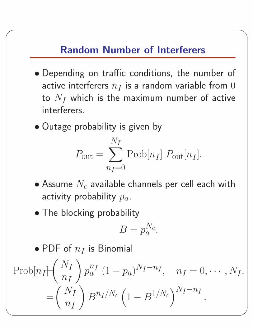
Random Number of Interferers
• Depending on traffic conditions, the number ofactive interferers nI is a random variable from 0to NI which is the maximum number of activeinterferers.
• Outage probability is given by
Pout =
NI∑
nI=0
Prob[nI ] Pout[nI ].
• Assume Nc available channels per cell each withactivity probability pa.
• The blocking probability
B = pNca .
• PDF of nI is Binomial
Prob[nI ]=
(NInI
)pnIa (1− pa)NI−nI , nI = 0, · · · , NI .
=
(NInI
)BnI/Nc
(1−B1/Nc
)NI−nI.
'
&
$
%
Outline - Part III: Co-Channel Interference
1. Co-Channel Interference (CCI) Analysis
• Effect of Shadowing
• Effect of Multipath Fading
– Single Interferer
– Multiple Interferers
– Minimum Desired Signal Requirement
– Random Number of Interferers
2. CCI Mitigation
• Diversity Combining
• Optimum Combining/Smart Antennas
• Optimized MIMO Systems in Presence of CCI
'
&
$
%
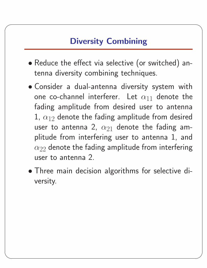
Diversity Combining
• Reduce the effect via selective (or switched) an-tenna diversity combining techniques.
• Consider a dual-antenna diversity system withone co-channel interferer. Let α11 denote thefading amplitude from desired user to antenna1, α12 denote the fading amplitude from desireduser to antenna 2, α21 denote the fading am-plitude from interfering user to antenna 1, andα22 denote the fading amplitude from interferinguser to antenna 2.
• Three main decision algorithms for selective di-versity.
'
&
$
%
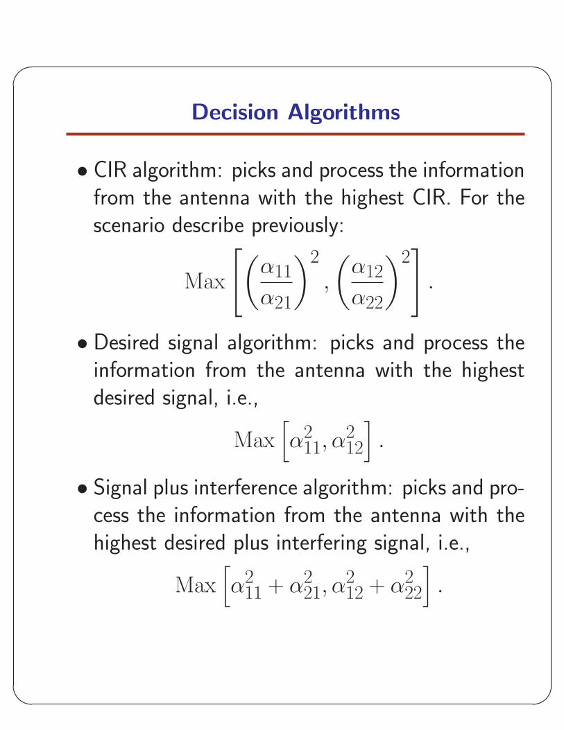
Decision Algorithms
• CIR algorithm: picks and process the informationfrom the antenna with the highest CIR. For thescenario describe previously:
Max
[(α11
α21
)2
,
(α12
α22
)2]
.
• Desired signal algorithm: picks and process theinformation from the antenna with the highestdesired signal, i.e.,
Max[α2
11, α212
].
• Signal plus interference algorithm: picks and pro-cess the information from the antenna with thehighest desired plus interfering signal, i.e.,
Max[α2
11 + α221, α
212 + α2
22
].
'
&
$
%
Interference Mitigation
•More advanced interference mitigation techniques
– Optimum combining
– Optimized MIMO systems

'
&
$
%
General Outline
• Part 0: Background, Motivation, and Goals.
• Part I: Some Basics.
• Part II: Diversity Systems.
• Part III: Co-Channel Interference.
• Part IV: Multi-Hop CommunicationSystems.
'
&
$
%
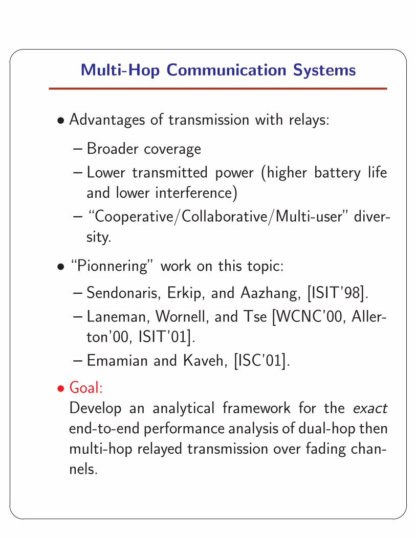
Multi-Hop Communication Systems
• Advantages of transmission with relays:
– Broader coverage
– Lower transmitted power (higher battery lifeand lower interference)
– “Cooperative/Collaborative/Multi-user” diver-sity.
• “Pionnering” work on this topic:
– Sendonaris, Erkip, and Aazhang, [ISIT’98].
– Laneman, Wornell, and Tse [WCNC’00, Aller-ton’00, ISIT’01].
– Emamian and Kaveh, [ISC’01].
• Goal:Develop an analytical framework for the exactend-to-end performance analysis of dual-hop thenmulti-hop relayed transmission over fading chan-nels.
'
&
$
%
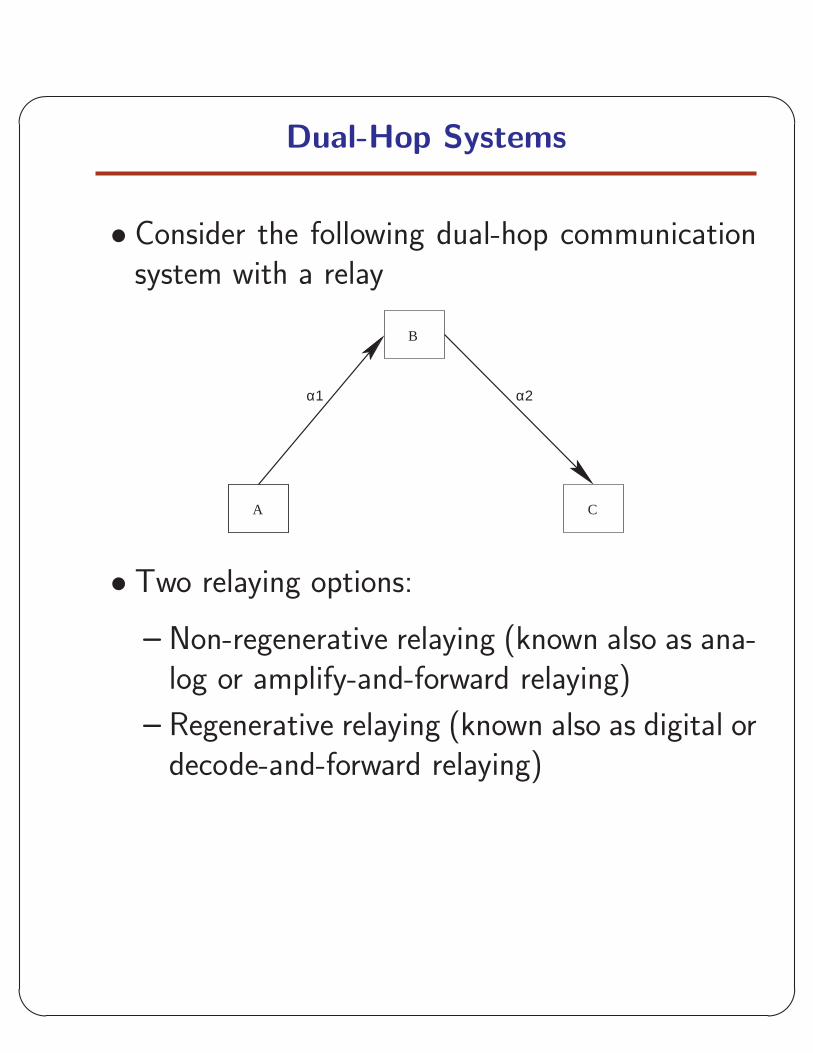
Dual-Hop Systems
• Consider the following dual-hop communicationsystem with a relay
CA
B
α2α1
• Two relaying options:
– Non-regenerative relaying (known also as ana-log or amplify-and-forward relaying)
– Regenerative relaying (known also as digital ordecode-and-forward relaying)
'
&
$
%
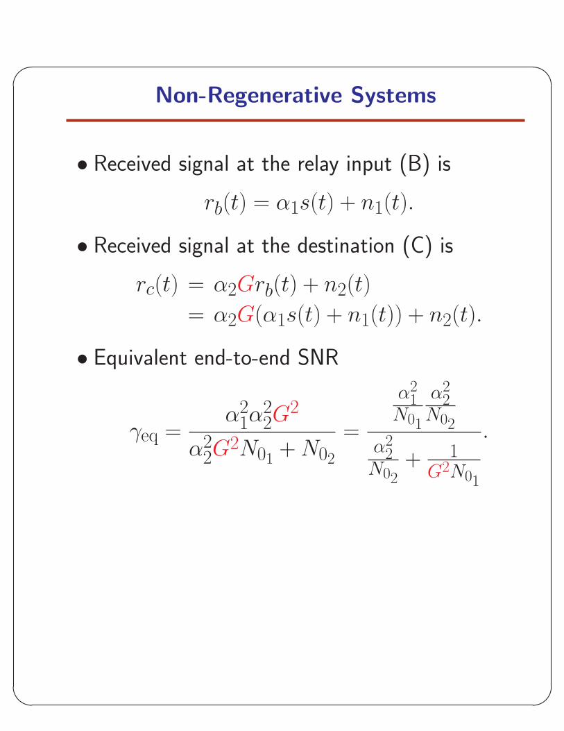
Non-Regenerative Systems
• Received signal at the relay input (B) is
rb(t) = α1s(t) + n1(t).
• Received signal at the destination (C) is
rc(t) = α2Grb(t) + n2(t)
= α2G(α1s(t) + n1(t)) + n2(t).
• Equivalent end-to-end SNR
γeq =α2
1α22G
2
α22G
2N01+ N02
=
α21
N01
α22
N02
α22
N02+ 1
G2N01
.
'
&
$
%
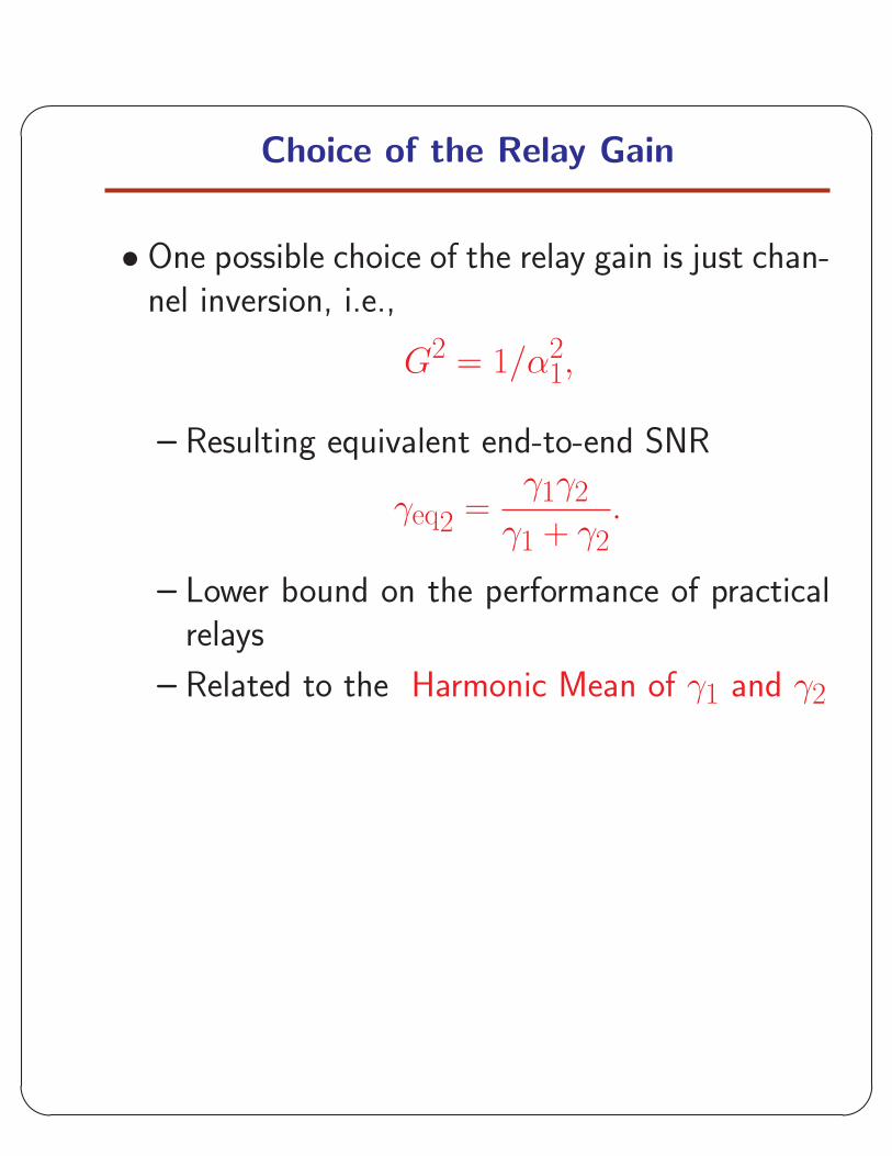
Choice of the Relay Gain
• One possible choice of the relay gain is just chan-nel inversion, i.e.,
G2 = 1/α21,
– Resulting equivalent end-to-end SNR
γeq2 =γ1γ2
γ1 + γ2.
– Lower bound on the performance of practicalrelays
– Related to the Harmonic Mean of γ1 and γ2
'
&
$
%
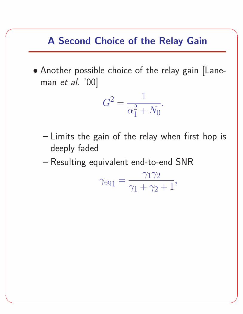
A Second Choice of the Relay Gain
• Another possible choice of the relay gain [Lane-man et al. ’00]
G2 =1
α21 + N0
.
– Limits the gain of the relay when first hop isdeeply faded
– Resulting equivalent end-to-end SNR
γeq1 =γ1γ2
γ1 + γ2 + 1,
'
&
$
%
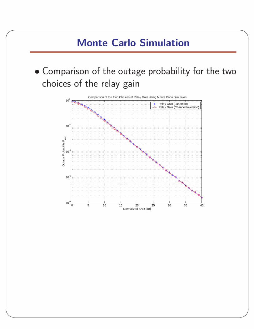
Monte Carlo Simulation
• Comparison of the outage probability for the twochoices of the relay gain
0 5 10 15 20 25 30 35 4010
−4
10−3
10−2
10−1
100
Normalized SNR [dB]
Out
age
Pro
babi
lity
Pou
t
Comparison of the Two Choices of Relay Gain Using Monte Carlo Simulaion
Relay Gain (Laneman)Relay Gain (Channel Inversion)
'
&
$
%
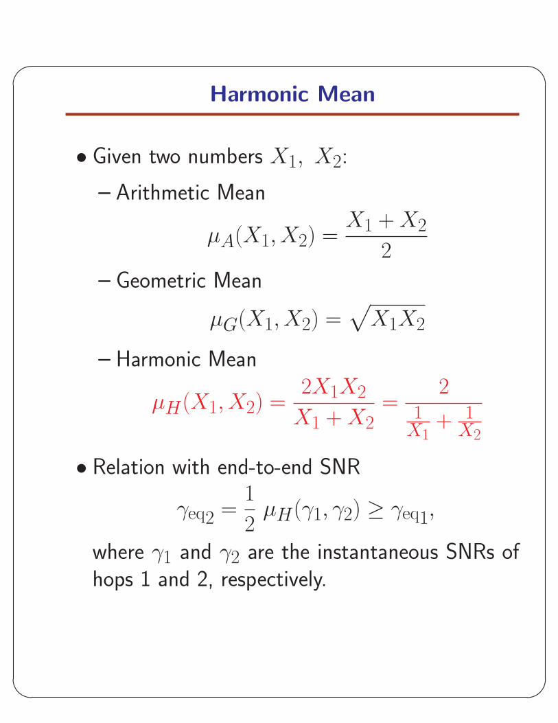
Harmonic Mean
• Given two numbers X1, X2:
– Arithmetic Mean
µA(X1, X2) =X1 + X2
2
– Geometric Mean
µG(X1, X2) =√
X1X2
– Harmonic Mean
µH(X1, X2) =2X1X2
X1 + X2=
21
X1+ 1
X2
• Relation with end-to-end SNR
γeq2 =1
2µH(γ1, γ2) ≥ γeq1,
where γ1 and γ2 are the instantaneous SNRs ofhops 1 and 2, respectively.
'
&
$
%
Harmonic Mean of Exponential Variates
• Theorem :Let X1 and X2 be two independent exponentialvariates with parameters β1 and β2 respectively.Then, the PDF of X = µH(X1, X2), pX(x), isgiven by
pX(x)=1
2β1β2xe−
x2(β1+β2)
[(β1 + β2√
β1β2
)K1
(x√
β1β2
)
+2K0
(x√
β1β2
)]U(x),
where Ki(·) is the ith order modified Besselfunction of the second kind and U(·) is the unitstep function.
• The CDF and MGF of the harmonic mean of twoindependent exponential variates are also avail-able in closed-form.
'
&
$
%
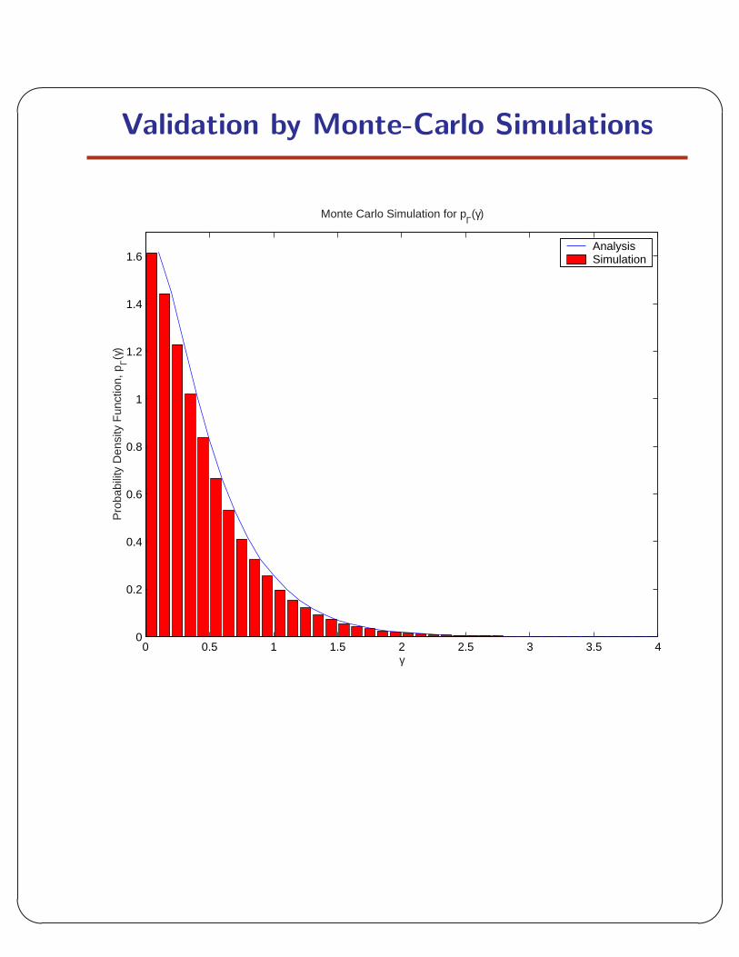
Validation by Monte-Carlo Simulations
0 0.5 1 1.5 2 2.5 3 3.5 40
0.2
0.4
0.6
0.8
1
1.2
1.4
1.6
Monte Carlo Simulation for pΓ(γ)
Pro
babi
lity
Den
sity
Fun
ctio
n, p
Γ(γ)
γ
Analysis Simulation
'
&
$
%
Derivation of the CDF of X = µH(X1, X2)
• Let
Z =1
X=
1
2
(1
X1+
1
X2
).
• The CDF of X, PX(x), is given by
PX(x) = Pr (X < x)
= Pr
(1
X>
1
x
)= Pr
(Z >
1
x
)
= 1− Pr
(Z <
1
x
)= 1− PZ
(1
x
),
where PZ(·) is the CDF of Z.
'
&
$
%
Derivation of the CDF of X = µH(X1, X2)(Continued)
• If X is an exponential random variable with pa-rameter β then the MGF of Y = 1/X can beshown to be given by
MY (s) = E[e−sY
]= 2
√βs K1
(2√
βs)
.
• Using the differentiation property of the Laplacetransform, PZ(z) can be written as
PZ(z) = L−1(MZ(s)
s
)
= 1− L−1(2√
β1β2K1
(2√
β1s)
K1
(2√
β2s))|z=1
x,
which is a tabulated inverse Laplace transformleading to
PX(x)=1− PZ
(1
x
)
=1− x√
β1β2e−x
2(β1+β2)K1
(x√
β1β2
).
'
&
$
%
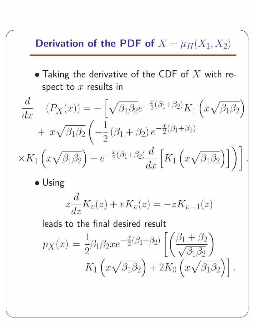
Derivation of the PDF of X = µH(X1, X2)
• Taking the derivative of the CDF of X with re-spect to x results in
d
dx(PX(x)) = −
[√β1β2e
−x2(β1+β2)K1
(x√
β1β2
)
+ x√
β1β2
(−1
2(β1 + β2) e−
x2(β1+β2)
×K1
(x√
β1β2
)+ e−
x2(β1+β2)
d
dx
[K1
(x√
β1β2
)])].
• Using
zd
dzKv(z) + vKv(z) = −zKv−1(z)
leads to the final desired result
pX(x) =1
2β1β2xe−
x2(β1+β2)
[(β1 + β2√
β1β2
)
K1
(x√
β1β2
)+ 2K0
(x√
β1β2
)].
'
&
$
%
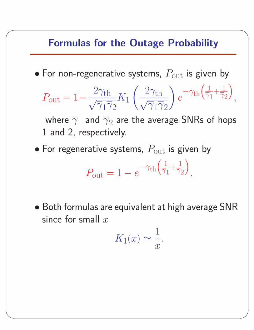
Formulas for the Outage Probability
• For non-regenerative systems, Pout is given by
Pout = 1− 2γth√γ1γ2
K1
(2γth√γ1γ2
)e−γth
(1γ1
+ 1γ2
),
where γ1 and γ2 are the average SNRs of hops1 and 2, respectively.
• For regenerative systems, Pout is given by
Pout = 1− e−γth
(1γ1
+ 1γ2
).
• Both formulas are equivalent at high average SNRsince for small x
K1(x) ' 1
x.
'
&
$
%
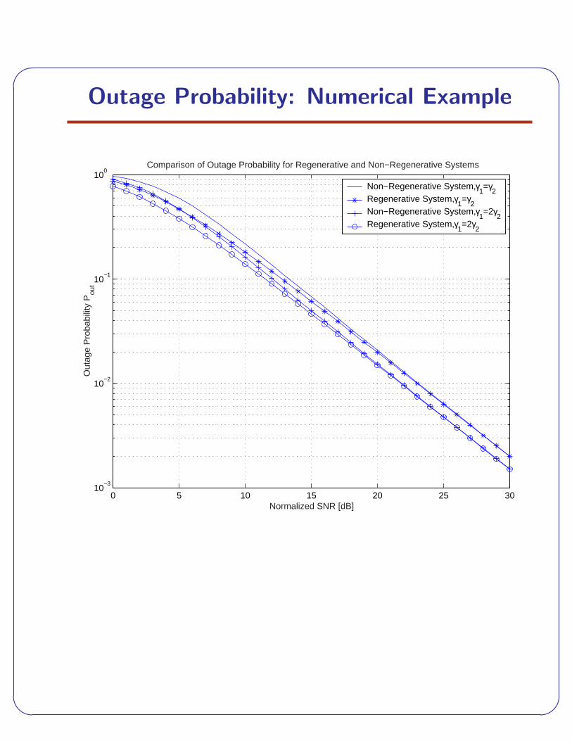
Outage Probability: Numerical Example
0 5 10 15 20 25 3010
−3
10−2
10−1
100
Normalized SNR [dB]
Out
age
Pro
babi
lity
Pou
t
Comparison of Outage Probability for Regenerative and Non−Regenerative Systems
Non−Regenerative System,γ1=γ
2Regenerative System,γ
1=γ
2Non−Regenerative System,γ
1=2γ
2Regenerative System,γ
1=2γ
2
'
&
$
%
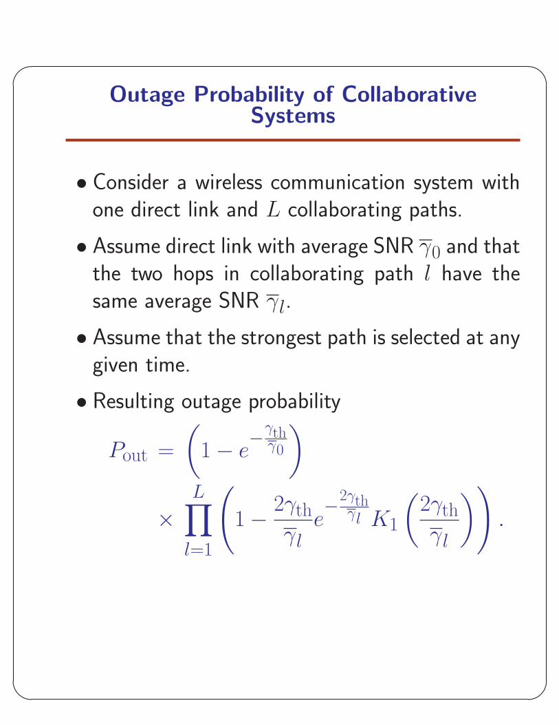
Outage Probability of CollaborativeSystems
• Consider a wireless communication system withone direct link and L collaborating paths.
• Assume direct link with average SNR γ0 and thatthe two hops in collaborating path l have thesame average SNR γl.
• Assume that the strongest path is selected at anygiven time.
• Resulting outage probability
Pout =
(1− e
−γthγ0
)
×L∏
l=1
(1− 2γth
γle−2γth
γl K1
(2γth
γl
)).
'
&
$
%
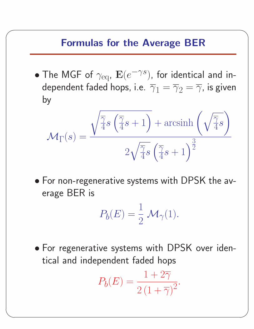
Formulas for the Average BER
• The MGF of γeq, E(e−γs), for identical and in-dependent faded hops, i.e. γ1 = γ2 = γ, is givenby
MΓ(s) =
√γ4s
(γ4s + 1
)+ arcsinh
(√γ4s
)
2√
γ4s
(γ4s + 1
)32
• For non-regenerative systems with DPSK the av-erage BER is
Pb(E) =1
2Mγ(1).
• For regenerative systems with DPSK over iden-tical and independent faded hops
Pb(E) =1 + 2γ
2 (1 + γ)2.
'
&
$
%
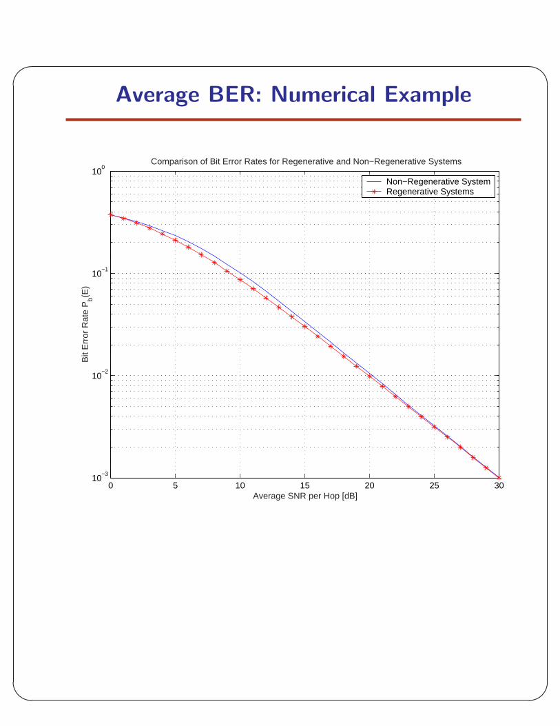
Average BER: Numerical Example
0 5 10 15 20 25 3010
−3
10−2
10−1
100
Average SNR per Hop [dB]
Bit
Err
or R
ate
Pb(E
)
Comparison of Bit Error Rates for Regenerative and Non−Regenerative Systems
Non−Regenerative SystemRegenerative Systems
'
&
$
%
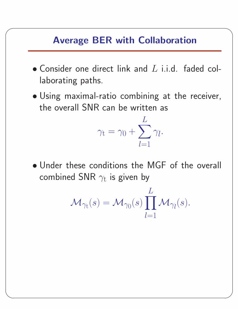
Average BER with Collaboration
• Consider one direct link and L i.i.d. faded col-laborating paths.
• Using maximal-ratio combining at the receiver,the overall SNR can be written as
γt = γ0 +
L∑
l=1
γl.
• Under these conditions the MGF of the overallcombined SNR γt is given by
Mγt(s) = Mγ0(s)
L∏
l=1
Mγl(s).
'
&
$
%
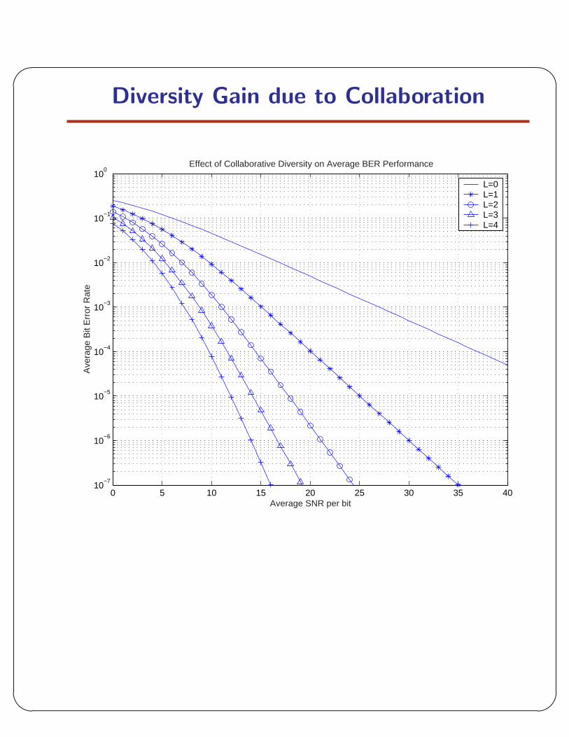
Diversity Gain due to Collaboration
0 5 10 15 20 25 30 35 4010
−7
10−6
10−5
10−4
10−3
10−2
10−1
100
Effect of Collaborative Diversity on Average BER Performance
Ave
rage
Bit
Err
or R
ate
Average SNR per bit
L=0L=1L=2L=3L=4
'
&
$
%
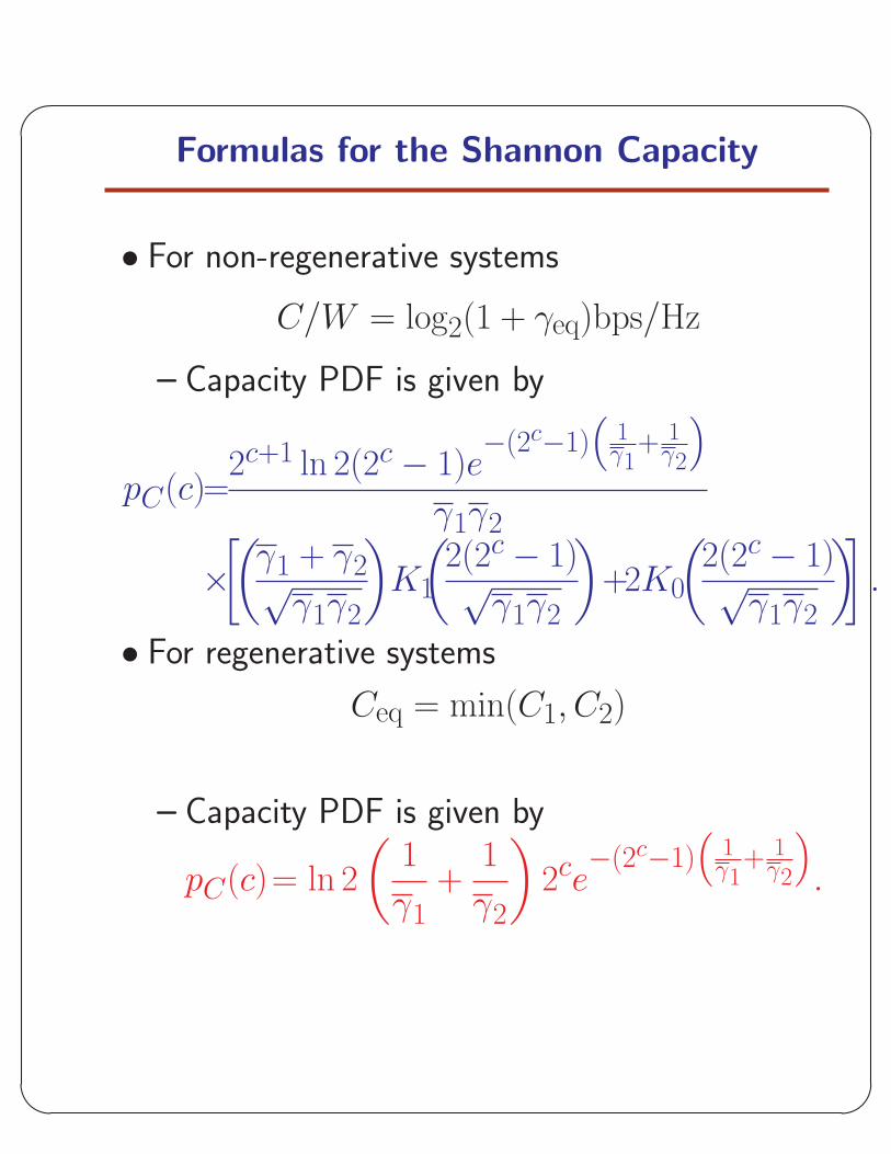
Formulas for the Shannon Capacity
• For non-regenerative systems
C/W = log2(1 + γeq)bps/Hz
– Capacity PDF is given by
pC(c)=2c+1 ln 2(2c − 1)e
−(2c−1)(
1γ1
+ 1γ2
)
γ1γ2
×[(
γ1 + γ2√γ1γ2
)K1
(2(2c − 1)√
γ1γ2
)+2K0
(2(2c − 1)√
γ1γ2
)].
• For regenerative systems
Ceq = min(C1, C2)
– Capacity PDF is given by
pC(c)= ln 2
(1
γ1+
1
γ2
)2ce
−(2c−1)(
1γ1
+ 1γ2
).
'
&
$
%
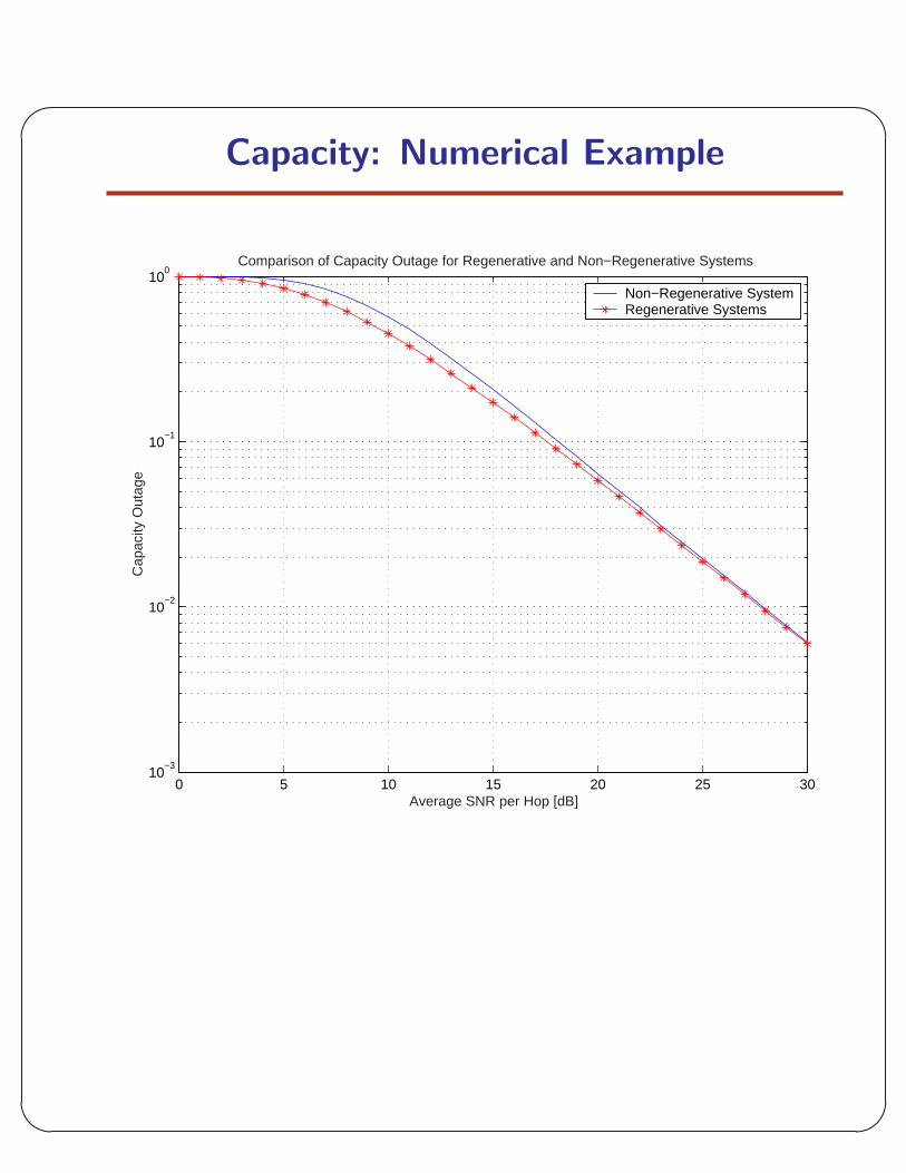
Capacity: Numerical Example
0 5 10 15 20 25 3010
−3
10−2
10−1
100
Average SNR per Hop [dB]
Cap
acity
Out
age
Comparison of Capacity Outage for Regenerative and Non−Regenerative Systems
Non−Regenerative SystemRegenerative Systems
'
&
$
%
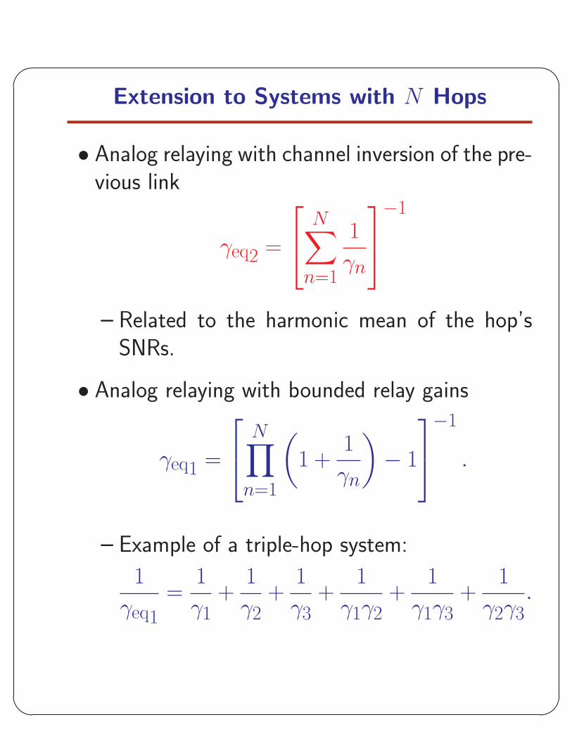
Extension to Systems with N Hops
• Analog relaying with channel inversion of the pre-vious link
γeq2 =
N∑
n=1
1
γn
−1
– Related to the harmonic mean of the hop’sSNRs.
• Analog relaying with bounded relay gains
γeq1 =
N∏
n=1
(1 +
1
γn
)− 1
−1
.
– Example of a triple-hop system:
1
γeq1=
1
γ1+
1
γ2+
1
γ3+
1
γ1γ2+
1
γ1γ3+
1
γ2γ3.
'
&
$
%
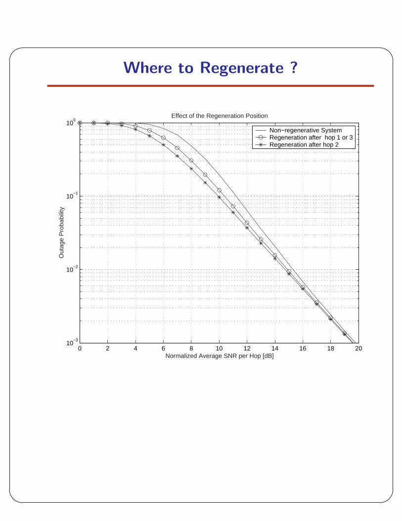
Where to Regenerate ?
0 2 4 6 8 10 12 14 16 18 2010
−3
10−2
10−1
100
Effect of the Regeneration Position
Normalized Average SNR per Hop [dB]
Out
age
Pro
babi
lity
Non−regenerative SystemRegeneration after hop 1 or 3Regeneration after hop 2
'
&
$
%
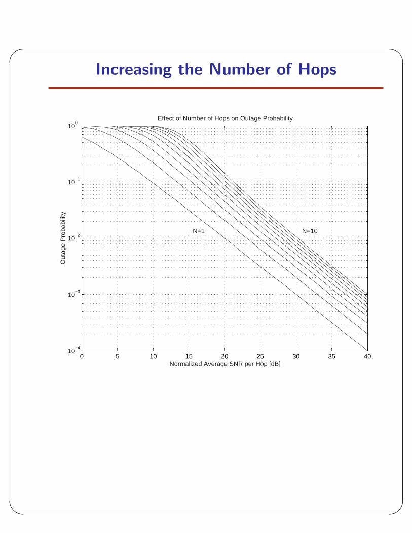
Increasing the Number of Hops
0 5 10 15 20 25 30 35 4010
−4
10−3
10−2
10−1
100
Effect of Number of Hops on Outage Probability
Normalized Average SNR per Hop [dB]
Out
age
Pro
babi
lity
N=1 N=10
'
&
$
%
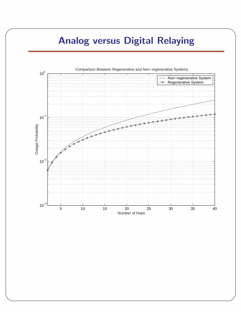
Analog versus Digital Relaying
5 10 15 20 25 30 35 4010
−3
10−2
10−1
100
Number of Hops
Out
age
Pro
babi
lity
Comparison Between Regenerative and Non−regenerative Systems
Non−regenerative SystemRegenerative System
'
&
$
%
Other Topics of Interest
• Analog relaying with “fixed” relay gain.
• Variable-power and/or variable rate relays.
• Latency and delay associated with multi-hop sys-tems.
• Global optimization versus local optimization.
• Power consumption and fairness issues.
Recommended