Parameter Uncertainty
April 2017
2
© 2017 Casualty Actuarial Society, Canadian Institute of Actuaries, and Society of Actuaries
Parameter Uncertainty
Caveat and Disclaimer The opinions expressed and conclusions reached by the authors are their own and do not represent any official position or opinion of the Society of Actuaries or its members. The Society of Actuaries makes no representation or warranty to the accuracy of the information. Copyright ©2017 All rights reserved by the Casualty Actuarial Society, Canadian Institute of Actuaries, and Society of Actuaries
SPONSORS
CAS/CIA/SOA Joint Risk Management Research Committee CAS/CIA/SOA Joint Risk Management Section
AUTHORS
Brian Hartman, PhD, ASA Robert Richardson, PhD, ASA Rylan Bateman
3
© 2017 Casualty Actuarial Society, Canadian Institute of Actuaries, and Society of Actuaries
TABLE OF CONTENTS
Section 1: Literature Review ..................................................................................................................................... 4
Section 2: Life Case Study.......................................................................................................................................... 6 2.1 ACTUAL-TO-TABULAR RATIO ................................................................................................................................... 6
2.1.1 POSTERIOR DISTRIBUTION FOR VARYING SAMPLE SIZES ................................................................. 8 2.1.2 SINGLE PREMIUM IMMEDIATE ANNUITY ........................................................................................ 10 2.1.3 EXTENSIONS ...................................................................................................................................... 11
2.2 MODELING THE MORTALITY RATES DIRECTLY ..................................................................................................... 12 2.2.1 SINGLE MORTALITY ........................................................................................................................... 12 2.2.2 ENTIRE MORTALITY CURVE .............................................................................................................. 15 2.2.3 SINGLE PREMIUM IMMEDIATE ANNUITY ........................................................................................ 17
2.3 TAIL MEASURES ................................................................................................................................................. 19 2.4 CONCLUSION ..................................................................................................................................................... 20
Section 3: Health Case Study ................................................................................................................................... 21 3.1 MODELS ............................................................................................................................................................. 21
3.1.1 ORDINARY LEAST SQUARES ................................................................................................................... 21 3.1.2 BAYESIAN REGRESSION .......................................................................................................................... 21 3.1.3 SPIKE AND SLAB ...................................................................................................................................... 22
3.2 DATA ILLUSTRATION .......................................................................................................................................... 23 3.3 PREDICTION COMPARISON ................................................................................................................................... 26
3.3.1 Parameter estimates ....................................................................................................................... 26 3.3.2 Predictions of new observations ...................................................................................................... 27
3.4 CONCLUSION ..................................................................................................................................................... 27
Section 4: Property/Casualty Case Study ................................................................................................................. 28 4.1 DATA ................................................................................................................................................................... 28 4.2 MODELS ............................................................................................................................................................. 28 4.3 RESULTS ............................................................................................................................................................. 29
4.3.1 POISSON REGRESSION ........................................................................................................................... 29 4.3.2 NEGATIVE BINOMIAL REGRESSION ....................................................................................................... 31
4.4 CONCLUSION ..................................................................................................................................................... 32
Section 5: Conclusion .............................................................................................................................................. 32
Section 6: References .............................................................................................................................................. 33
4
© 2017 Casualty Actuarial Society, Canadian Institute of Actuaries, and Society of Actuaries
Parameter Uncertainty
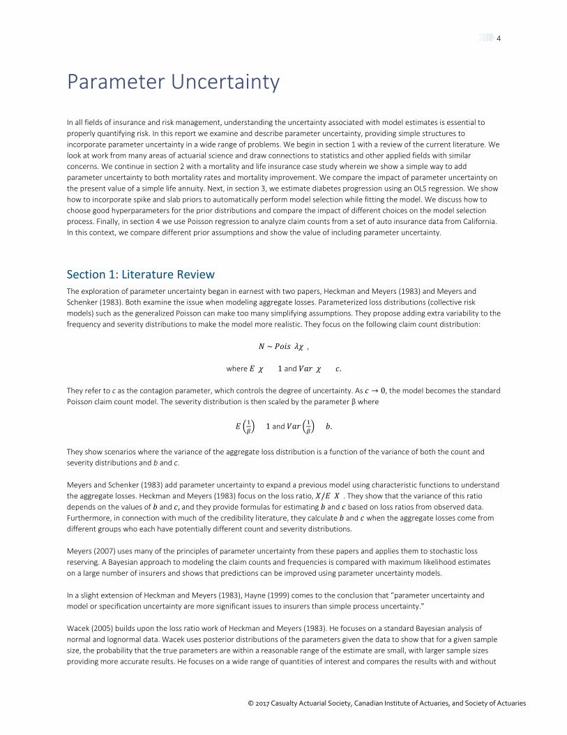
In all fields of insurance and risk management, understanding the uncertainty associated with model estimates is essential to properly quantifying risk. In this report we examine and describe parameter uncertainty, providing simple structures to incorporate parameter uncertainty in a wide range of problems. We begin in section 1 with a review of the current literature. We look at work from many areas of actuarial science and draw connections to statistics and other applied fields with similar concerns. We continue in section 2 with a mortality and life insurance case study wherein we show a simple way to add parameter uncertainty to both mortality rates and mortality improvement. We compare the impact of parameter uncertainty on the present value of a simple life annuity. Next, in section 3, we estimate diabetes progression using an OLS regression. We show how to incorporate spike and slab priors to automatically perform model selection while fitting the model. We discuss how to choose good hyperparameters for the prior distributions and compare the impact of different choices on the model selection process. Finally, in section 4 we use Poisson regression to analyze claim counts from a set of auto insurance data from California. In this context, we compare different prior assumptions and show the value of including parameter uncertainty.
Section 1: Literature Review The exploration of parameter uncertainty began in earnest with two papers, Heckman and Meyers (1983) and Meyers and Schenker (1983). Both examine the issue when modeling aggregate losses. Parameterized loss distributions (collective risk models) such as the generalized Poisson can make too many simplifying assumptions. They propose adding extra variability to the frequency and severity distributions to make the model more realistic. They focus on the following claim count distribution:
𝑁𝑁 ~ 𝑃𝑃𝑃𝑃𝑃𝑃𝑃𝑃(𝜆𝜆𝜆𝜆),
where 𝐸𝐸(𝜆𝜆) = 1 and 𝑉𝑉𝑉𝑉𝑉𝑉(𝜆𝜆) = 𝑐𝑐.
They refer to c as the contagion parameter, which controls the degree of uncertainty. As 𝑐𝑐 → 0, the model becomes the standard Poisson claim count model. The severity distribution is then scaled by the parameter β where
𝐸𝐸 �1𝛽𝛽� = 1 and 𝑉𝑉𝑉𝑉𝑉𝑉 �1
𝛽𝛽� = 𝑏𝑏.
They show scenarios where the variance of the aggregate loss distribution is a function of the variance of both the count and severity distributions and b and c.
Meyers and Schenker (1983) add parameter uncertainty to expand a previous model using characteristic functions to understand the aggregate losses. Heckman and Meyers (1983) focus on the loss ratio, 𝑋𝑋/𝐸𝐸(𝑋𝑋). They show that the variance of this ratio depends on the values of 𝑏𝑏 and 𝑐𝑐, and they provide formulas for estimating 𝑏𝑏 and 𝑐𝑐 based on loss ratios from observed data. Furthermore, in connection with much of the credibility literature, they calculate 𝑏𝑏 and 𝑐𝑐 when the aggregate losses come from different groups who each have potentially different count and severity distributions.
Meyers (2007) uses many of the principles of parameter uncertainty from these papers and applies them to stochastic loss reserving. A Bayesian approach to modeling the claim counts and frequencies is compared with maximum likelihood estimates on a large number of insurers and shows that predictions can be improved using parameter uncertainty models.
In a slight extension of Heckman and Meyers (1983), Hayne (1999) comes to the conclusion that “parameter uncertainty and model or specification uncertainty are more significant issues to insurers than simple process uncertainty."
Wacek (2005) builds upon the loss ratio work of Heckman and Meyers (1983). He focuses on a standard Bayesian analysis of normal and lognormal data. Wacek uses posterior distributions of the parameters given the data to show that for a given sample size, the probability that the true parameters are within a reasonable range of the estimate are small, with larger sample sizes providing more accurate results. He focuses on a wide range of quantities of interest and compares the results with and without
5
© 2017 Casualty Actuarial Society, Canadian Institute of Actuaries, and Society of Actuaries
parameter uncertainty. In addition to loss ratios, he examines aggregate excess reinsurance, downside risk measures and commissions.
Borowicz and Norman (2006) focus on aggregate losses above a certain level (the extreme values). They assume the count (N) follows a Poisson distribution and severity (X) follows a generalized Pareto distribution. Three different methods are compared to quantify the parameter uncertainty: (1) Fisher's information, (2) bootstrapping and (3) Bayesian methods. Diers, Eling and Linde (2013) build upon that work, using the same three methods to quantify parameter uncertainty. They also explore the effect of sample size on the results. They focus on aggregate claims and separate the large claims from the attritional claims. The large claims are given a Poisson count and Pareto severity while the attritional claims are lumped in one gamma distribution. They compare how some significant quantities of interest are affected by the parameter uncertainty in both a one-year time frame and a five-year time frame, the most significant of which is VaR99.5.
In a similar vein, Gerrard and Tsanakas (2011) model failure where failure is a specific risk factor exceeding a certain threshold. The losses are random, and the risk capital is also random and initially held to be a percentile of the loss distribution. The probability of insolvency is calculated for a variety of loss distributions under maximum likelihood estimates. To decrease the probability of insolvency in the presence of uncertainty, they explore setting the risk capital to a higher percentile of the loss distribution than actually desired. The main argument of the paper is that instead of setting the percentile higher, one can introduce parameter uncertainty via a Bayesian prior into the loss distribution and then use the desired percentile. The prior is integrated out when the percentile is calculated.
Bignozzi and Tsanakas (2015) focus more generally on how the risk measures are affected by parameter uncertainty. As expected, the required capital to stay within certain risk requirements is larger when parameter uncertainty is present. They focus on location-scale families and show that the adjustment to the risk measure is mathematically convenient. They use a measure called the residual risk, which, for a given risk metric such as VaR, capital estimator and loss random variable, returns a value that evaluates the risk in the presence of additional uncertainty. A good goal is for this to be 0. They show that when a loss distribution is used with a Bayesian prior integrated out, the capital required for the residual risk to be zero is larger than when parameter uncertainty is not required.
Taking a broader view, Cairns (2000) discusses model and parameter uncertainty. The approach is inherently Bayesian, and the parameter uncertainty is incorporated through a prior on the parameters. He reviews three statistical methods of model uncertainty: (1) comparing model fit using a criterion such as AIC or BIC, (2) finding the model from a set of models with the highest posterior probability and (3) finding the posterior distribution of the parameters of all the models along with the posterior probabilities of the specific models. He includes two examples. In the first, he simulates stochastic interest rates using random rates of interest with continuous force between time points. He then uses two models, an i.i.d. normal model and an AR(1) model, and compares them using all three methods of model uncertainty. In his second example, he simulates data from a lognormal distribution and compares 10 gamma likelihoods with different scale parameters. From the resulting fit he then calculates the amount needed to hold in reserve to avoid ruin and determines that adding parameter uncertainty requires more to be held in reserve.
Additionally, many papers look at parameter uncertainty in specific applications. Cairns, Blake and Dowd (2006) is the first in a long list of papers exploring parameter uncertainty in stochastic mortality. Mortality is modeled as a logistic regression with parameters that vary stochastically across time. Parameter uncertainty comes from priors on the mean and the variance terms of the logistic regression parameters, with a multivariate normal on the mean vector and inverse Wishart on the covariance matrix. The difference between the point estimates of the two models (with or without parameter uncertainty) is minimal.
In financial risk management, Hartman and Heaton (2011) examine the impact of parameter uncertainty in asset simulation, especially regime-switching models. They use a standard Bayesian model to add parameter uncertainty and a Bayesian nonparametric model to account for model uncertainty. They found that incorporating parameter uncertainty had a much bigger impact on the risk measures than the model uncertainty. These models were further extended beyond regime-switching models to GARCH and stochastic volatility models in Hartman and Groendyke (2013).
In health insurance, Fellingham, Kottas and Hartman (2015) examine the impact of parameter and model uncertainty on group health claim prediction. They find that a model that incorporates both types of uncertainty outperforms other models when
6
© 2017 Casualty Actuarial Society, Canadian Institute of Actuaries, and Society of Actuaries
predicting future year claims. The improvement is greatest when predicting claims for a new group that is not in the current data set.
In property and casualty insurance, Shi and Hartman (2016) examine the impact of parameter uncertainty in loss reserving. They build on the classic chain-ladder model using Bayesian regression. They also show how to incorporate information from similar lines of business to improve predictive accuracy. Venter and Sahasrabuddhe (2015) review various ways to incorporate parameter uncertainty (which they call parameter risk).
A number of actuarial applications have been analyzed using parameter uncertainty in the framework of Bayesian methodology. Shi, Basu and Meyers (2012) model multivariate reserving from multiple lines of insurance. They use a Bayesian log-normal model and directly model the pairwise correlations between the different lines. They show that by employing valuation actuaries' prior knowledge they can significantly improve prediction over the model without parameter uncertainty. Meyers (1999) also estimates correlation between multivariate outcome variables using parameter uncertainty in predictive modeling.
The idea of parameter uncertainty being used to make more realistic models is employed in various other fields as well, namely, science and engineering (e.g., Kitanidis (1986), Wood and Rodriguez-Iturbe (1975), Beck and Katafygiotis (1998)). An entire field in statistics has arisen to address the nature and degree of parameter uncertainty seen in certain physical models. This field has been termed uncertainty quantification (Smith, 2013). Much of the parameter uncertainty that will arise in actuarial applications can be addressed using Bayesian methodology. References such as Gelman et al. (2014) and Marin and Robert (2007) share insight on how to set up Bayesian models, how to analyze them and how to answer questions using them.
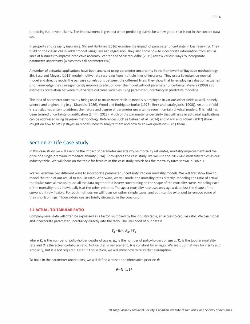
Section 2: Life Case Study In this case study we will examine the impact of parameter uncertainty on mortality estimates, mortality improvement and the price of a single premium immediate annuity (SPIA). Throughout the case study, we will use the 2012 IAM mortality tables as our industry table. We will focus on the table for females in this case study, which has the mortality rates shown in Table 1.
We will examine two different ways to incorporate parameter uncertainty into our mortality models. We will first show how to model the ratio of our actual to tabular rates. Afterward, we will model the mortality rates directly. Modeling the ratio of actual to tabular rates allows us to use all the data together but is very constraining on the shape of the mortality curve. Modeling each of the mortality rates individually is at the other extreme. The age 𝑥𝑥 mortality rate uses only age 𝑥𝑥 data, but the shape of the curve is entirely flexible. For both methods we will focus on rather simple cases, and both can be extended to remove some of their shortcomings. Those extensions are briefly discussed in the conclusion.
2.1 ACTUAL-TO-TABULAR RATIO Company-level data will often be expressed as a factor multiplied by the industry table, an actual-to-tabular ratio. We can model and incorporate parameter uncertainty directly into the ratio. The likelihood of our data is
𝑌𝑌𝑎𝑎~𝐵𝐵𝑃𝑃𝐵𝐵(𝐸𝐸𝑎𝑎,𝜃𝜃𝑇𝑇𝑎𝑎),
where 𝑌𝑌𝑎𝑎 is the number of policyholder deaths of age 𝑉𝑉, 𝐸𝐸𝑎𝑎 is the number of policyholders of age 𝑉𝑉, 𝑇𝑇𝑎𝑎 is the tabular mortality rate and 𝜃𝜃 is the actual-to-tabular ratio. Notice that in our scenario, 𝜃𝜃 is constant for all ages. We set it up that way for clarity and simplicity, but it is not required. Later in this section, we will show how to relax that assumption.
To build in the parameter uncertainty, we will define a rather noninformative prior on 𝜃𝜃:
𝜃𝜃~𝑁𝑁(1, 12).
7
© 2017 Casualty Actuarial Society, Canadian Institute of Actuaries, and Society of Actuaries
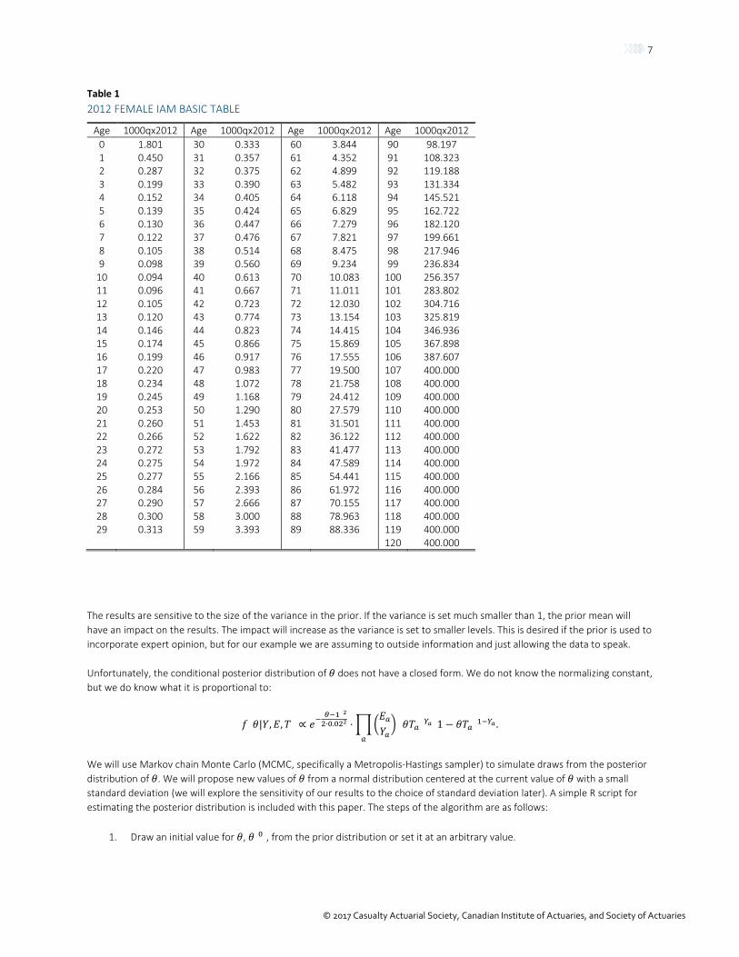
Table 1 2012 FEMALE IAM BASIC TABLE
Age 1000qx2012 Age 1000qx2012 Age 1000qx2012 Age 1000qx2012 0 1.801 30 0.333 60 3.844 90 98.197 1 0.450 31 0.357 61 4.352 91 108.323 2 0.287 32 0.375 62 4.899 92 119.188 3 0.199 33 0.390 63 5.482 93 131.334 4 0.152 34 0.405 64 6.118 94 145.521 5 0.139 35 0.424 65 6.829 95 162.722 6 0.130 36 0.447 66 7.279 96 182.120 7 0.122 37 0.476 67 7.821 97 199.661 8 0.105 38 0.514 68 8.475 98 217.946 9 0.098 39 0.560 69 9.234 99 236.834
10 0.094 40 0.613 70 10.083 100 256.357 11 0.096 41 0.667 71 11.011 101 283.802 12 0.105 42 0.723 72 12.030 102 304.716 13 0.120 43 0.774 73 13.154 103 325.819 14 0.146 44 0.823 74 14.415 104 346.936 15 0.174 45 0.866 75 15.869 105 367.898 16 0.199 46 0.917 76 17.555 106 387.607 17 0.220 47 0.983 77 19.500 107 400.000 18 0.234 48 1.072 78 21.758 108 400.000 19 0.245 49 1.168 79 24.412 109 400.000 20 0.253 50 1.290 80 27.579 110 400.000 21 0.260 51 1.453 81 31.501 111 400.000 22 0.266 52 1.622 82 36.122 112 400.000 23 0.272 53 1.792 83 41.477 113 400.000 24 0.275 54 1.972 84 47.589 114 400.000 25 0.277 55 2.166 85 54.441 115 400.000 26 0.284 56 2.393 86 61.972 116 400.000 27 0.290 57 2.666 87 70.155 117 400.000 28 0.300 58 3.000 88 78.963 118 400.000 29 0.313 59 3.393 89 88.336 119 400.000
120 400.000
The results are sensitive to the size of the variance in the prior. If the variance is set much smaller than 1, the prior mean will have an impact on the results. The impact will increase as the variance is set to smaller levels. This is desired if the prior is used to incorporate expert opinion, but for our example we are assuming to outside information and just allowing the data to speak.
Unfortunately, the conditional posterior distribution of 𝜃𝜃 does not have a closed form. We do not know the normalizing constant, but we do know what it is proportional to:
𝑓𝑓(𝜃𝜃|𝑌𝑌,𝐸𝐸,𝑇𝑇) ∝ 𝑒𝑒−(𝜃𝜃−1)22⋅0.022 ⋅��
𝐸𝐸𝑎𝑎𝑌𝑌𝑎𝑎� (𝜃𝜃𝑇𝑇𝑎𝑎)𝑌𝑌𝑎𝑎(1 − 𝜃𝜃𝑇𝑇𝑎𝑎)1−𝑌𝑌𝑎𝑎
𝑎𝑎
.
We will use Markov chain Monte Carlo (MCMC, specifically a Metropolis-Hastings sampler) to simulate draws from the posterior distribution of 𝜃𝜃. We will propose new values of 𝜃𝜃 from a normal distribution centered at the current value of 𝜃𝜃 with a small standard deviation (we will explore the sensitivity of our results to the choice of standard deviation later). A simple R script for estimating the posterior distribution is included with this paper. The steps of the algorithm are as follows:
1. Draw an initial value for 𝜃𝜃, 𝜃𝜃(0), from the prior distribution or set it at an arbitrary value.
8
© 2017 Casualty Actuarial Society, Canadian Institute of Actuaries, and Society of Actuaries
2. Until you reach the desired number of iterations, for each iteration 𝑃𝑃
a. Propose a new value of 𝜃𝜃,𝜃𝜃∗, drawn from the proposal distribution, 𝑁𝑁�𝜃𝜃(𝑖𝑖−1), 0.0352�.
b. Calculate the Metropolis-Hastings acceptance probability, 𝛼𝛼, using the following equation:
𝛼𝛼 =𝑓𝑓(𝜃𝜃∗|𝑌𝑌,𝐸𝐸,𝑇𝑇)
𝑓𝑓�𝜃𝜃(𝑖𝑖−1)�𝑌𝑌,𝐸𝐸,𝑇𝑇�.
Note that even though we don’t know the normalizing constant of the posterior distribution, they will cancel in the acceptance probability.
c. Draw 𝑈𝑈 ∼ 𝑈𝑈𝐵𝐵𝑃𝑃𝑓𝑓(0,1). If 𝛼𝛼 > 𝑈𝑈, then accept the proposed value and 𝜃𝜃(𝑖𝑖) = 𝜃𝜃∗. Otherwise, you reject the proposed value and 𝜃𝜃(𝑖𝑖) = 𝜃𝜃(𝑖𝑖−1).
3. Use the draws (after removing the first few for burn-in) to understand the posterior distribution of 𝜃𝜃.
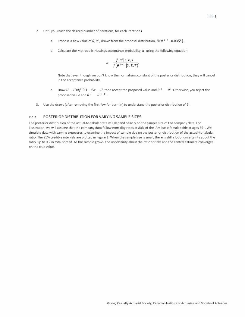
2.1.1 POSTERIOR DISTRIBUTION FOR VARYING SAMPLE SIZES
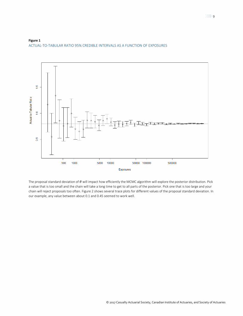
The posterior distribution of the actual-to-tabular rate will depend heavily on the sample size of the company data. For illustration, we will assume that the company data follow mortality rates at 80% of the IAM basic female table at ages 65+. We simulate data with varying exposures to examine the impact of sample size on the posterior distribution of the actual-to-tabular ratio. The 95% credible intervals are plotted in Figure 1. When the sample size is small, there is still a lot of uncertainty about the ratio, up to 0.2 in total spread. As the sample grows, the uncertainty about the ratio shrinks and the central estimate converges on the true value.
9
© 2017 Casualty Actuarial Society, Canadian Institute of Actuaries, and Society of Actuaries
Figure 1 ACTUAL-TO-TABULAR RATIO 95% CREDIBLE INTERVALS AS A FUNCTION OF EXPOSURES
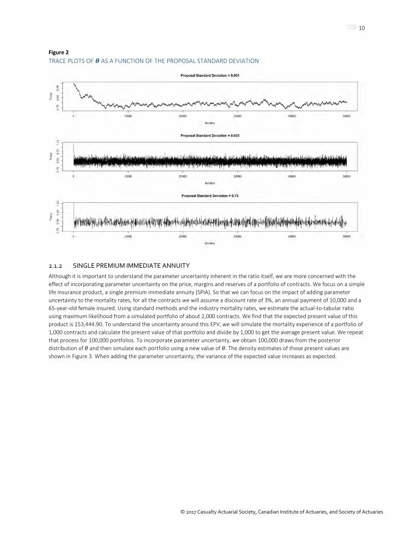
The proposal standard deviation of 𝜃𝜃 will impact how efficiently the MCMC algorithm will explore the posterior distribution. Pick a value that is too small and the chain will take a long time to get to all parts of the posterior. Pick one that is too large and your chain will reject proposals too often. Figure 2 shows several trace plots for different values of the proposal standard deviation. In our example, any value between about 0.1 and 0.45 seemed to work well.
10
© 2017 Casualty Actuarial Society, Canadian Institute of Actuaries, and Society of Actuaries
Figure 2 TRACE PLOTS OF 𝜽𝜽 AS A FUNCTION OF THE PROPOSAL STANDARD DEVIATION
2.1.2 SINGLE PREMIUM IMMEDIATE ANNUITY
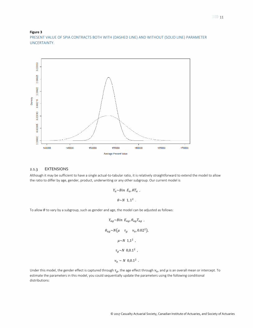
Although it is important to understand the parameter uncertainty inherent in the ratio itself, we are more concerned with the effect of incorporating parameter uncertainty on the price, margins and reserves of a portfolio of contracts. We focus on a simple life insurance product, a single premium immediate annuity (SPIA). So that we can focus on the impact of adding parameter uncertainty to the mortality rates, for all the contracts we will assume a discount rate of 3%, an annual payment of 10,000 and a 65-year-old female insured. Using standard methods and the industry mortality rates, we estimate the actual-to-tabular ratio using maximum likelihood from a simulated portfolio of about 2,000 contracts. We find that the expected present value of this product is 153,444.90. To understand the uncertainty around this EPV, we will simulate the mortality experience of a portfolio of 1,000 contracts and calculate the present value of that portfolio and divide by 1,000 to get the average present value. We repeat that process for 100,000 portfolios. To incorporate parameter uncertainty, we obtain 100,000 draws from the posterior distribution of 𝜃𝜃 and then simulate each portfolio using a new value of 𝜃𝜃. The density estimates of those present values are shown in Figure 3. When adding the parameter uncertainty, the variance of the expected value increases as expected.
11
© 2017 Casualty Actuarial Society, Canadian Institute of Actuaries, and Society of Actuaries
Figure 3 PRESENT VALUE OF SPIA CONTRACTS BOTH WITH (DASHED LINE) AND WITHOUT (SOLID LINE) PARAMETER UNCERTAINTY.
2.1.3 EXTENSIONS
Although it may be sufficient to have a single actual-to-tabular ratio, it is relatively straightforward to extend the model to allow the ratio to differ by age, gender, product, underwriting or any other subgroup. Our current model is
𝑌𝑌𝑎𝑎~𝐵𝐵𝑃𝑃𝐵𝐵(𝐸𝐸𝑎𝑎,𝜃𝜃𝑇𝑇𝑎𝑎),
𝜃𝜃~𝑁𝑁(1, 12).
To allow 𝜃𝜃 to vary by a subgroup, such as gender and age, the model can be adjusted as follows:
𝑌𝑌𝑎𝑎𝑎𝑎~𝐵𝐵𝑃𝑃𝐵𝐵(𝐸𝐸𝑎𝑎𝑎𝑎,𝜃𝜃𝑎𝑎𝑎𝑎𝑇𝑇𝑎𝑎𝑎𝑎),
𝜃𝜃𝑎𝑎𝑎𝑎~𝑁𝑁�𝜇𝜇 + 𝜏𝜏𝑎𝑎 + 𝜈𝜈𝑎𝑎, 0.022�,
𝜇𝜇~𝑁𝑁(1,12),
𝜏𝜏𝑎𝑎~𝑁𝑁(0,0.12),
𝜈𝜈𝑎𝑎 ∼ 𝑁𝑁(0,0.12).
Under this model, the gender effect is captured through 𝜏𝜏𝑎𝑎, the age effect through 𝜈𝜈𝑎𝑎, and 𝜇𝜇 is an overall mean or intercept. To estimate the parameters in this model, you could sequentially update the parameters using the following conditional distributions:
12
© 2017 Casualty Actuarial Society, Canadian Institute of Actuaries, and Society of Actuaries
𝑓𝑓(𝜃𝜃|𝜇𝜇,𝑌𝑌,𝐸𝐸,𝑇𝑇) ∝ 𝑒𝑒−(𝜃𝜃−1)22⋅0.022 ⋅��
𝐸𝐸𝑎𝑎𝑎𝑎𝑌𝑌𝑎𝑎𝑎𝑎
� �𝜃𝜃𝑇𝑇𝑎𝑎𝑎𝑎�𝑌𝑌𝑎𝑎𝑎𝑎�1− 𝜃𝜃𝑇𝑇𝑎𝑎𝑎𝑎�
1−𝑌𝑌𝑎𝑎𝑎𝑎
𝑎𝑎,𝑎𝑎
,
𝜇𝜇|𝜃𝜃,𝑌𝑌,𝐸𝐸,𝑇𝑇, 𝜏𝜏, 𝜈𝜈 ~ 𝑁𝑁�1 +
∑ 𝜃𝜃 − 𝜏𝜏𝑎𝑎 − 𝜈𝜈𝑎𝑎𝑎𝑎𝑎𝑎0.022
1 + 10.022
,1
1 + 10.022
�,
𝜏𝜏|𝜃𝜃,𝑌𝑌,𝐸𝐸,𝑇𝑇, 𝜇𝜇, 𝜈𝜈 ~ 𝑁𝑁�1
0.12 +∑ 𝜃𝜃 − 𝜇𝜇 − 𝜈𝜈𝑎𝑎𝑎𝑎𝑎𝑎
0.0221
0.12 + 10.022
,1
10.12 + 1
0.022�,
𝜈𝜈|𝜃𝜃,𝑌𝑌,𝐸𝐸,𝑇𝑇, 𝜇𝜇, 𝜏𝜏 ~ 𝑁𝑁�1
0.12 +∑ 𝜃𝜃 − 𝜇𝜇 − 𝜏𝜏𝑎𝑎𝑎𝑎𝑎𝑎
0.0221
0.12 + 10.022
,1
10.12 + 1
0.022�.
We would only need to use a Metropolis-Hastings step on 𝜃𝜃; the rest can be directly drawn from known distributions. The model can be further extended to include other categories, interactions between the groups (allowing the gender effect to differ by age) and correlations between the ages (to constrain the 𝜈𝜈𝑎𝑎 to change smoothly across ages), among many other options.
2.2 MODELING THE MORTALITY RATES DIRECTLY To incorporate parameter uncertainty directly and be able to update the industry estimates with our internal data, we will assume that the mortality rates follow a Beta distribution a priori:
𝑞𝑞𝑥𝑥 ~ 𝐵𝐵𝑒𝑒𝐵𝐵𝑉𝑉(𝛼𝛼,𝛽𝛽),
𝑓𝑓(𝑞𝑞𝑥𝑥) =Γ(𝛼𝛼)Γ(𝛽𝛽)Γ(𝛼𝛼 + 𝛽𝛽) 𝑞𝑞𝑥𝑥
𝛼𝛼−1(1 − 𝑞𝑞𝑥𝑥)𝛽𝛽−1, 𝛼𝛼 > 0, 𝛽𝛽 > 0.
We chose the Beta distribution because it is constrained to be between zero and one and it is the conjugate prior when dealing with binomial responses. Assuming that your data have X successes (in this case, deaths) out of a possible 𝐸𝐸 trials (lives of age x), then the posterior distribution will also follow a Beta distribution with the following parameters:
𝑞𝑞𝑥𝑥|𝐸𝐸,𝑋𝑋 ~ 𝐵𝐵𝑒𝑒𝐵𝐵𝑉𝑉(𝛼𝛼 + 𝑋𝑋,𝛽𝛽 + 𝐸𝐸 − 𝑋𝑋).
2.2.1 SINGLE MORTALITY
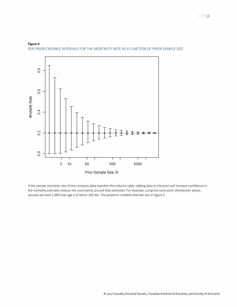
The prior distribution is centered on the industry table value. The spread of the distribution is determined by the parameter 𝑁𝑁, which is the “prior sample size.” The prior is given weight equal to a data set of size 𝑁𝑁 with 𝑁𝑁𝑞𝑞𝑥𝑥𝑖𝑖𝑖𝑖𝑖𝑖 deaths where 𝑞𝑞𝑥𝑥𝑖𝑖𝑖𝑖𝑖𝑖 is the industry table mortality rate. If the industry data come from a population that perfectly matches your company data (for all the characteristics that affect mortality), 𝑁𝑁 could be equal to the number of exposures at each year in the industry study. More likely, the industry data will differ from your book in meaningful ways, so you will need to reduce 𝑁𝑁. At the other extreme, if the populations differ so greatly that you do not want to use much of the industry data at all, you can make 𝑁𝑁 very small or even 0. The prior sample size can also vary by age, gender or any other characteristic you prefer. As N gets larger, the prior distribution becomes narrower, meaning that you are more confident that the mortality rate is close to the industry rate. The more confident you are about the prior (industry) mortality rate, the smaller the impact of the data. For a simple example, we will examine a single mortality rate (Figure 4) where the industry mortality rate is 0.2. When 𝑁𝑁 is 50, the credible interval (the set of reasonable values for the true mortality rate) is still rather large, about 0.2 in total width. When 𝑁𝑁 grows to many thousands, the range of plausible values becomes very small.
13
© 2017 Casualty Actuarial Society, Canadian Institute of Actuaries, and Society of Actuaries
Figure 4 95% PRIOR CREDIBLE INTERVALS FOR THE MORTALITY RATE AS A FUNCTION OF PRIOR SAMPLE SIZE.
If the sample mortality rate of the company data matches the industry table, adding data to the prior will increase confidence in the mortality estimate (reduce the uncertainty around that estimate). For example, using the same prior distribution above, assume we have 1,000 lives age x of which 200 die. The posterior credible intervals are in Figure 5.
14
© 2017 Casualty Actuarial Society, Canadian Institute of Actuaries, and Society of Actuaries
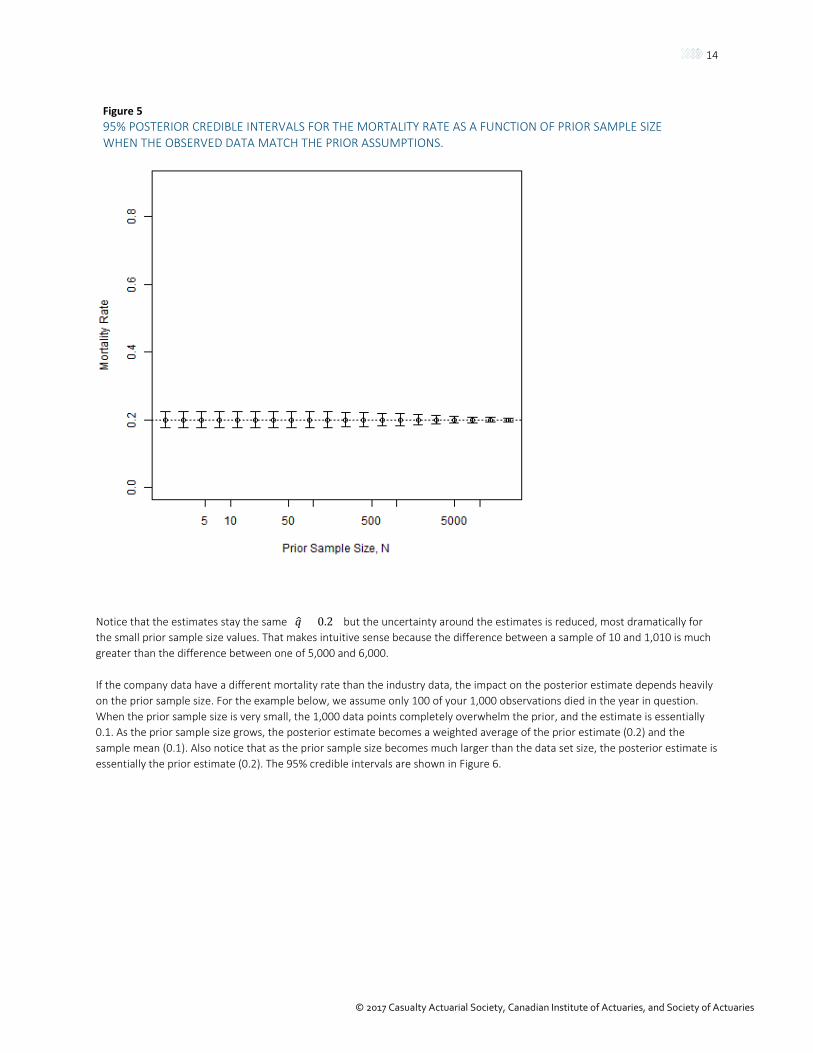
Figure 5 95% POSTERIOR CREDIBLE INTERVALS FOR THE MORTALITY RATE AS A FUNCTION OF PRIOR SAMPLE SIZE WHEN THE OBSERVED DATA MATCH THE PRIOR ASSUMPTIONS.
Notice that the estimates stay the same (𝑞𝑞� = 0.2) but the uncertainty around the estimates is reduced, most dramatically for the small prior sample size values. That makes intuitive sense because the difference between a sample of 10 and 1,010 is much greater than the difference between one of 5,000 and 6,000.
If the company data have a different mortality rate than the industry data, the impact on the posterior estimate depends heavily on the prior sample size. For the example below, we assume only 100 of your 1,000 observations died in the year in question. When the prior sample size is very small, the 1,000 data points completely overwhelm the prior, and the estimate is essentially 0.1. As the prior sample size grows, the posterior estimate becomes a weighted average of the prior estimate (0.2) and the sample mean (0.1). Also notice that as the prior sample size becomes much larger than the data set size, the posterior estimate is essentially the prior estimate (0.2). The 95% credible intervals are shown in Figure 6.
15
© 2017 Casualty Actuarial Society, Canadian Institute of Actuaries, and Society of Actuaries
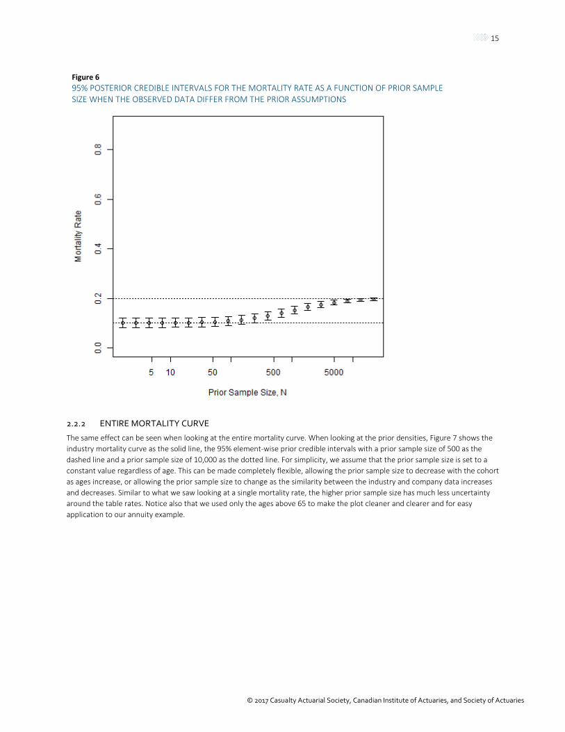
Figure 6 95% POSTERIOR CREDIBLE INTERVALS FOR THE MORTALITY RATE AS A FUNCTION OF PRIOR SAMPLE SIZE WHEN THE OBSERVED DATA DIFFER FROM THE PRIOR ASSUMPTIONS
2.2.2 ENTIRE MORTALITY CURVE
The same effect can be seen when looking at the entire mortality curve. When looking at the prior densities, Figure 7 shows the industry mortality curve as the solid line, the 95% element-wise prior credible intervals with a prior sample size of 500 as the dashed line and a prior sample size of 10,000 as the dotted line. For simplicity, we assume that the prior sample size is set to a constant value regardless of age. This can be made completely flexible, allowing the prior sample size to decrease with the cohort as ages increase, or allowing the prior sample size to change as the similarity between the industry and company data increases and decreases. Similar to what we saw looking at a single mortality rate, the higher prior sample size has much less uncertainty around the table rates. Notice also that we used only the ages above 65 to make the plot cleaner and clearer and for easy application to our annuity example.
16
© 2017 Casualty Actuarial Society, Canadian Institute of Actuaries, and Society of Actuaries
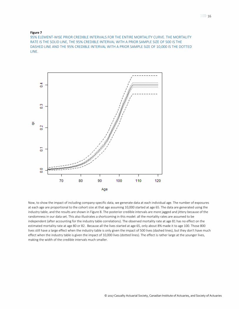
Figure 7 95% ELEMENT-WISE PRIOR CREDIBLE INTERVALS FOR THE ENTIRE MORTALITY CURVE. THE MORTALITY RATE IS THE SOLID LINE, THE 95% CREDIBLE INTERVAL WITH A PRIOR SAMPLE SIZE OF 500 IS THE DASHED LINE AND THE 95% CREDIBLE INTERVAL WITH A PRIOR SAMPLE SIZE OF 10,000 IS THE DOTTED LINE.
Now, to show the impact of including company-specific data, we generate data at each individual age. The number of exposures at each age are proportional to the cohort size at that age assuming 10,000 started at age 65. The data are generated using the industry table, and the results are shown in Figure 8. The posterior credible intervals are more jagged and jittery because of the randomness in our data set. This also illustrates a shortcoming in this model: all the mortality rates are assumed to be independent (after accounting for the industry table correlations). The observed mortality rate at age 81 has no effect on the estimated mortality rate at age 80 or 82. Because all the lives started at age 65, only about 8% made it to age 100. Those 800 lives still have a large effect when the industry table is only given the impact of 500 lives (dashed lines), but they don't have much effect when the industry table is given the impact of 10,000 lives (dotted lines). The effect is rather large at the younger lives, making the width of the credible intervals much smaller.

17
© 2017 Casualty Actuarial Society, Canadian Institute of Actuaries, and Society of Actuaries
Figure 8 95% ELEMENT-WISE POSTERIOR CREDIBLE INTERVALS FOR THE ENTIRE MORTALITY CURVE. DATA DRAWN FROM THE MORTALITY TABLE ARE INCORPORATED. THE MORTALITY RATE IS THE SOLID LINE, THE 95% CREDIBLE INTERVAL WITH A PRIOR SAMPLE SIZE OF 500 IS THE DASHED LINE AND THE 95% CREDIBLE INTERVAL WITH A PRIOR SAMPLE SIZE OF 10,000 IS THE DOTTED LINE.
2.2.3 SINGLE PREMIUM IMMEDIATE ANNUITY
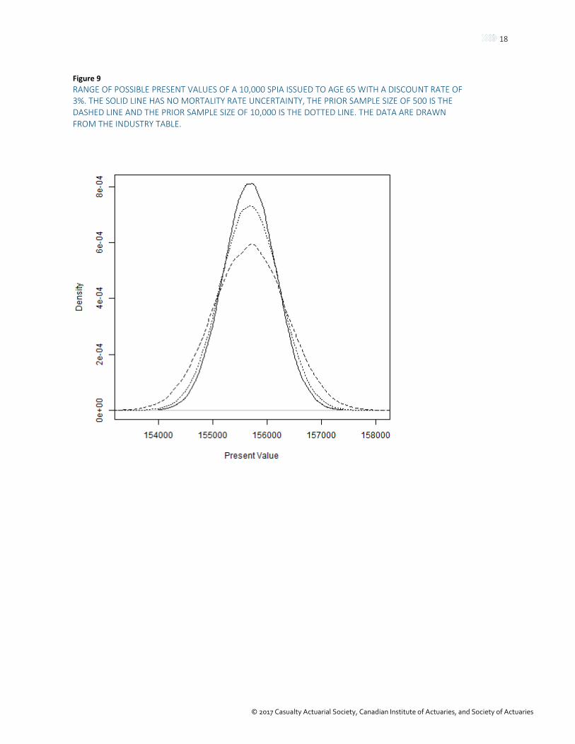
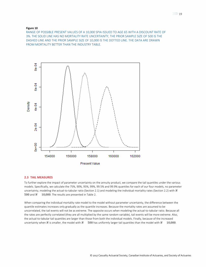
We now incorporate parameter uncertainty in the mortality rates, following the methodology in Section 2.2.2. In Figure 9 we compare the effect of parameter uncertainty on the present values when the 10,000 observed lives follow the industry mortality. In Figure 10, we show what happens when the observed lives’ mortality rates are 10% better. Note that in both these scenarios we are assuming no mortality improvement. We will incorporate mortality improvement in the next section.
As expected, when the company data follow the industry table, adding parameter uncertainty simply increases the uncertainty in the present values. The expected present value remains the same. But, when the company data have better mortality experience than the industry table, it will pull the present values up. The pull is greatest when the prior sample size is smallest. Notice also that the smaller prior sample size has the larger posterior uncertainty.
18
© 2017 Casualty Actuarial Society, Canadian Institute of Actuaries, and Society of Actuaries
Figure 9 RANGE OF POSSIBLE PRESENT VALUES OF A 10,000 SPIA ISSUED TO AGE 65 WITH A DISCOUNT RATE OF 3%. THE SOLID LINE HAS NO MORTALITY RATE UNCERTAINTY, THE PRIOR SAMPLE SIZE OF 500 IS THE DASHED LINE AND THE PRIOR SAMPLE SIZE OF 10,000 IS THE DOTTED LINE. THE DATA ARE DRAWN FROM THE INDUSTRY TABLE.
19
© 2017 Casualty Actuarial Society, Canadian Institute of Actuaries, and Society of Actuaries
Figure 10 RANGE OF POSSIBLE PRESENT VALUES OF A 10,000 SPIA ISSUED TO AGE 65 WITH A DISCOUNT RATE OF 3%. THE SOLID LINE HAS NO MORTALITY RATE UNCERTAINTY, THE PRIOR SAMPLE SIZE OF 500 IS THE DASHED LINE AND THE PRIOR SAMPLE SIZE OF 10,000 IS THE DOTTED LINE. THE DATA ARE DRAWN FROM MORTALITY BETTER THAN THE INDUSTRY TABLE.
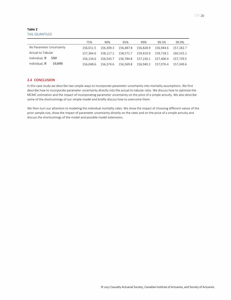
2.3 TAIL MEASURES To further explore the impact of parameter uncertainty on the annuity product, we compare the tail quantiles under the various models. Specifically, we calculate the 75%, 90%, 95%, 99%, 99.5% and 99.9% quantiles for each of our four models, no parameter uncertainty, modeling the actual-to-tabular ratio (Section 2.1) and modeling the individual mortality rates (Section 2.2) with 𝑁𝑁 =500 and 𝑁𝑁 = 10,000. The results are presented in Table 2.
When comparing the individual mortality rate model to the model without parameter uncertainty, the difference between the quantile estimates increases only gradually as the quantile increases. Because the mortality rates are assumed to be uncorrelated, the tail events will not be as extreme. The opposite occurs when modeling the actual-to-tabular ratio. Because all the rates are perfectly correlated (they are all multiplied by the same random variable), tail events will be more extreme. Also, the actual-to-tabular tail quantiles are larger than those from both the individual models. Finally, because of the increased uncertainty when 𝑁𝑁 is smaller, the model with 𝑁𝑁 = 500 has uniformly larger tail quantiles than the model with 𝑁𝑁 = 10,000.
20
© 2017 Casualty Actuarial Society, Canadian Institute of Actuaries, and Society of Actuaries
Table 2 TAIL QUANTILES
75% 90% 95% 99% 99.5% 99.9% No Parameter Uncertainty 156,011.5 156,309.3 156,487.8 156,828.9 156,944.6 157,182.7 Actual-to-Tabular 157,364.6 158,117.2 158,571.7 159,410.9 159,718.1 160,333.2 Individual, 𝑁𝑁 = 500 156,134.6 156,543.7 156,784.8 157,230.1 157,400.4 157,739.5 Individual, 𝑁𝑁 = 10,000 156,048.6 156,374.6 156,569.8 156,940.2 157,076.4 157,349.6
2.4 CONCLUSION In this case study we describe two simple ways to incorporate parameter uncertainty into mortality assumptions. We first describe how to incorporate parameter uncertainty directly into the actual-to-tabular ratio. We discuss how to optimize the MCMC estimation and the impact of incorporating parameter uncertainty on the price of a simple annuity. We also describe some of the shortcomings of our simple model and briefly discuss how to overcome them.
We then turn our attention to modeling the individual mortality rates. We show the impact of choosing different values of the prior sample size, show the impact of parameter uncertainty directly on the rates and on the price of a simple annuity and discuss the shortcomings of the model and possible model extensions.
21
© 2017 Casualty Actuarial Society, Canadian Institute of Actuaries, and Society of Actuaries
Section 3: Health Case Study As in other areas of insurance, predictive modeling plays a large role in health insurance. These models are used in underwriting, reserving and claims management. Many of these predictive models can be written as linear models or generalized linear models, depending on what is being predicted. A continuous response such as BMI can be modeled in a linear model as a function of variables such as weight and age. The probability an individual will lapse or renew a policy can be written as a logistic regression model using predictors such as age, sex and marital status. The relationship between the predictor variables and the outcomes may have uncertainty associated with them. Instead of using optimization methods to find point estimates and then asymptotic theory to develop distributions of the estimates, parameters uncertainty can be built into the estimation of the parameters by building a Bayesian model. We use a regression setting to compare models that incorporate parameter uncertainty with those that do not. We use a standard Bayesian regression model and a more advanced Bayesian regression model that will also incorporate uncertainty into the selection of the variables.
3.1 MODELS
3.1.1 ORDINARY LEAST SQUARES
Linear models are typically written as
𝑦𝑦𝑗𝑗 = 𝛽𝛽0 + 𝛽𝛽1𝑥𝑥1,𝑗𝑗 + 𝛽𝛽2𝑥𝑥2,𝑗𝑗 + ⋯+ 𝜖𝜖𝑗𝑗 ,
where 𝑦𝑦𝑗𝑗 is the observed data, 𝑥𝑥𝑖𝑖,𝑗𝑗 are the explanatory variables, 𝛽𝛽𝑖𝑖 represents the effect of the i-th variable on 𝑦𝑦𝑗𝑗 and 𝜖𝜖𝑗𝑗 are independent normal error terms. The 𝛽𝛽𝑖𝑖 coefficients represent the expected change in 𝑦𝑦𝑗𝑗 given a unit change in 𝑥𝑥𝑖𝑖,𝑗𝑗 when everything else remains unchanged.
Ordinary least squares (OLS) is a method that selects the parameters that minimize the sum of squared residuals. After the model is fit, a confidence interval can be constructed for each 𝛽𝛽𝑖𝑖 with an upper and lower bound. Using asymptotic properties, it is even possible to construct a distribution of the parameters after the model is fit. However, no uncertainty is included in the parameters at the time the parameters are estimated, so it is estimated as if it is a static, unchanging value that we simply do not know. Also, predictions are made without any uncertainty of the parameters. The advantages of OLS are that it is conceptually simple, easy to implement and computationally fast.
3.1.2 BAYESIAN REGRESSION
In Bayesian modeling, each parameter is given a prior that reflects the modeler’s belief in the distribution of possible values for the parameter. The impact of a variable may be well understood before the company data are collected or any models are fit. In that case, the prior distribution of the related parameters may be narrower (have a smaller spread). When there is limited prior knowledge, the prior distribution on the parameters will be very wide. The data will then update the prior, and the resulting distribution is called the posterior distribution. It will reflect the prior and the data, but the result is a distribution for the parameters, and it will account for uncertainty. This uncertainty will also be used in making predictions for new observations.
The regression equation in the Bayesian setting is equivalent to the OLS case. The prior distribution of the regression coefficients, 𝛽𝛽0,𝛽𝛽1, …, will be normal (N), and the prior distribution for the variance of 𝜖𝜖𝑖𝑖 will be inverse gamma (IG). These priors are chosen for computational convenience because the math involved to update these priors using the data is straightforward (the priors are conjugate). In model form, the priors are included in the model as follows:
𝑦𝑦𝑗𝑗 = 𝛽𝛽0 + �𝛽𝛽𝑖𝑖𝑥𝑥𝑖𝑖,𝑗𝑗 + 𝜖𝜖𝑗𝑗
𝑀𝑀
𝑖𝑖=1
, 𝑗𝑗 = 1, … ,𝐵𝐵,
𝜷𝜷~ 𝑁𝑁(𝝁𝝁,𝜎𝜎2𝚲𝚲), 𝑗𝑗 = 0, … ,𝑀𝑀,
𝜖𝜖𝑗𝑗 ~ 𝑁𝑁(0,𝜎𝜎2), 𝜎𝜎2 ~ 𝐼𝐼𝐼𝐼(𝑉𝑉, 𝑏𝑏),
22
© 2017 Casualty Actuarial Society, Canadian Institute of Actuaries, and Society of Actuaries
where 𝜷𝜷 and 𝝁𝝁 are vectors with 𝜷𝜷 = (𝛽𝛽0,𝛽𝛽1, … ,𝛽𝛽𝑀𝑀)′ and 𝝁𝝁 = (𝜇𝜇0, 𝜇𝜇1, … , 𝜇𝜇𝑀𝑀)′ , and 𝚲𝚲 is a matrix with prior variance and covariance values. This matrix could be diagonal where if Λ𝑖𝑖 represents the ith diagonal element, then the prior variance of 𝛽𝛽𝑖𝑖 would be 𝜎𝜎2Λ𝑖𝑖. The modeler will have to define the prior uncertainty by choosing values for 𝜇𝜇𝑖𝑖, Λ𝑖𝑖 , 𝑉𝑉 and 𝑏𝑏. Each 𝜇𝜇𝑖𝑖 represents the prior belief in the expected value for 𝛽𝛽𝑖𝑖 , and Λ𝑖𝑖 is chosen to be large when there is less certainty about what the value for 𝛽𝛽𝑖𝑖 is. The values for 𝑉𝑉 and 𝑏𝑏 should be chosen to represent the perceived variance of the response when the predictor variables are taken into account.
For example, suppose we are building a logistic regression model to predict whether or not an individual contracts a lung disease in the coming year. If a variable was included indicating whether or not the individual smoked, we would expect that an individual who smoked would have a higher probability of getting a lung disease, and so we would choose a prior that indicates this with a high amount of certainty. If another variable in the model was the size of the individual’s house, we may not know the effect, if there is one, so we would choose a prior that is wide to reflect a high amount of uncertainty involved. We will see later how these prior values affect the estimates and prediction intervals for the parameters and predictions.
3.1.3 SPIKE AND SLAB
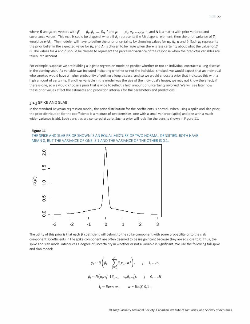
In the standard Bayesian regression model, the prior distribution for the coefficients is normal. When using a spike and slab prior, the prior distribution for the coefficients is a mixture of two densities, one with a small variance (spike) and one with a much wider variance (slab). Both densities are centered at zero. Such a prior will look like the density shown in Figure 11.
Figure 11 THE SPIKE AND SLAB PRIOR SHOWN IS AN EQUAL MIXTURE OF TWO NORMAL DENSITIES. BOTH HAVE MEAN 0, BUT THE VARIANCE OF ONE IS 1 AND THE VARIANCE OF THE OTHER IS 0.1.
The utility of this prior is that each 𝛽𝛽 coefficient will belong to the spike component with some probability or to the slab component. Coefficients in the spike component are often deemed to be insignificant because they are so close to 0. Thus, the spike and slab model introduces a degree of uncertainty in whether or not a variable is significant. We use the following full spike and slab model:
𝑦𝑦𝑗𝑗 ~ 𝑁𝑁�𝛽𝛽0 + �𝛽𝛽𝑖𝑖𝑥𝑥𝑖𝑖,𝑗𝑗 ,𝜎𝜎2𝑀𝑀
𝑖𝑖=1
� , 𝑗𝑗 = 1, … ,𝐵𝐵,
𝛽𝛽𝑖𝑖 ~ 𝑁𝑁�𝜇𝜇𝑖𝑖 , 𝜏𝜏𝑖𝑖2(1𝛿𝛿𝑙𝑙𝑖𝑖=1 + 𝑣𝑣0𝛿𝛿𝑙𝑙𝑖𝑖=0�, 𝑗𝑗 = 0, … ,𝑀𝑀,
𝑙𝑙𝑖𝑖 ~ 𝐵𝐵𝑒𝑒𝑉𝑉𝐵𝐵(𝑤𝑤), 𝑤𝑤 ~ 𝑈𝑈𝐵𝐵𝑃𝑃𝑓𝑓(0,1),
-3 -2 -1 0 1 2 3
23
© 2017 Casualty Actuarial Society, Canadian Institute of Actuaries, and Society of Actuaries
𝜎𝜎2 ~ 𝐼𝐼𝐼𝐼(𝑉𝑉𝜎𝜎 , 𝑏𝑏𝜎𝜎), 𝜏𝜏2 ~ 𝐼𝐼𝐼𝐼(𝑉𝑉𝜏𝜏, 𝑏𝑏𝜏𝜏).
The power of this model comes from the assignment variable 𝑙𝑙𝑖𝑖 which is one when the coefficient belongs to the slab and zero when the coefficient belongs to the spike, represented in the model by the Bernoulli distribution (Bern) with parameter 𝑤𝑤 having a standard uniform prior distribution (Unif). The posterior distribution is drawn using Markov chain Monte Carlo (MCMC) methods, which means that a new draw for 𝑙𝑙𝑖𝑖 is made for several iterations. If 90% of those draws are 𝑙𝑙𝑖𝑖 = 1, then we could say that there is a 90% probability that the coefficient is significantly different from zero. Additional details concerning the spike and slab prior, including more specific computational methods, can be found in Ishwaran and Rao (2005).
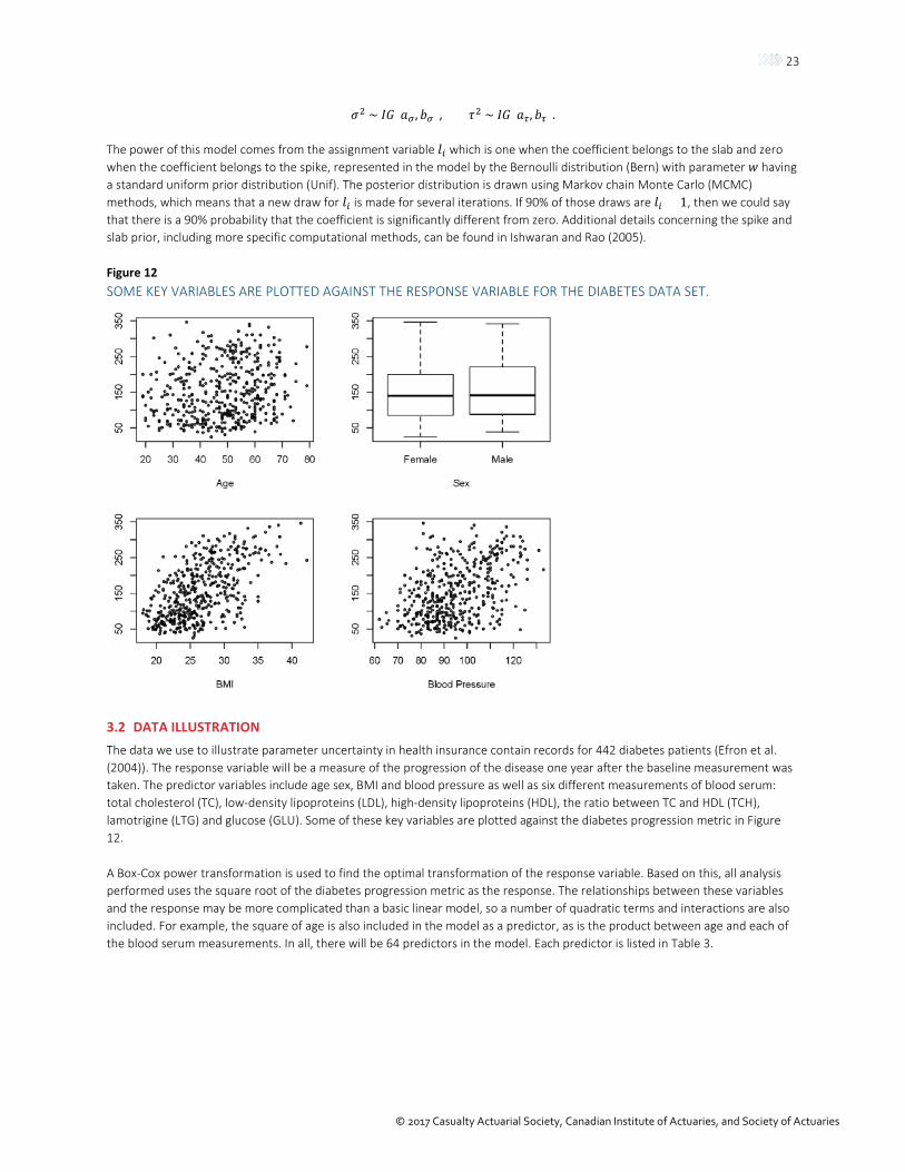
Figure 12 SOME KEY VARIABLES ARE PLOTTED AGAINST THE RESPONSE VARIABLE FOR THE DIABETES DATA SET.
3.2 DATA ILLUSTRATION The data we use to illustrate parameter uncertainty in health insurance contain records for 442 diabetes patients (Efron et al. (2004)). The response variable will be a measure of the progression of the disease one year after the baseline measurement was taken. The predictor variables include age sex, BMI and blood pressure as well as six different measurements of blood serum: total cholesterol (TC), low-density lipoproteins (LDL), high-density lipoproteins (HDL), the ratio between TC and HDL (TCH), lamotrigine (LTG) and glucose (GLU). Some of these key variables are plotted against the diabetes progression metric in Figure 12.
A Box-Cox power transformation is used to find the optimal transformation of the response variable. Based on this, all analysis performed uses the square root of the diabetes progression metric as the response. The relationships between these variables and the response may be more complicated than a basic linear model, so a number of quadratic terms and interactions are also included. For example, the square of age is also included in the model as a predictor, as is the product between age and each of the blood serum measurements. In all, there will be 64 predictors in the model. Each predictor is listed in Table 3.
24
© 2017 Casualty Actuarial Society, Canadian Institute of Actuaries, and Society of Actuaries
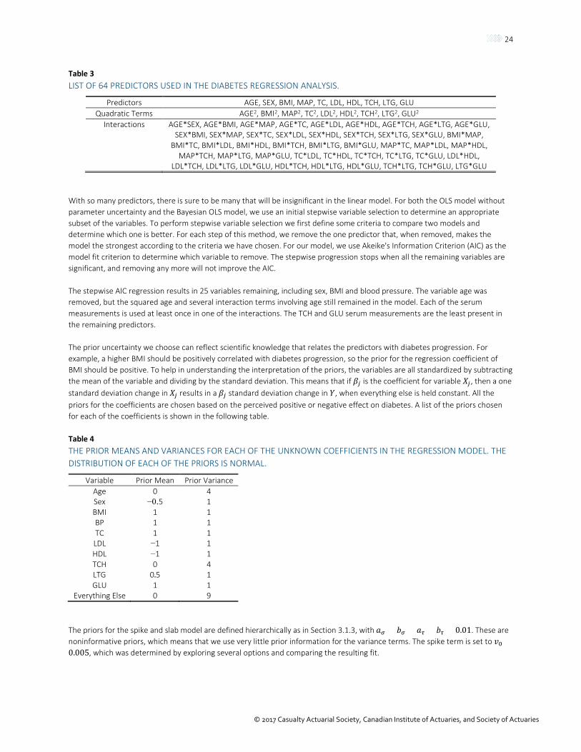
Table 3 LIST OF 64 PREDICTORS USED IN THE DIABETES REGRESSION ANALYSIS.
Predictors AGE, SEX, BMI, MAP, TC, LDL, HDL, TCH, LTG, GLU Quadratic Terms AGE2, BMI2, MAP2, TC2, LDL2, HDL2, TCH2, LTG2, GLU2
Interactions AGE*SEX, AGE*BMI, AGE*MAP, AGE*TC, AGE*LDL, AGE*HDL, AGE*TCH, AGE*LTG, AGE*GLU, SEX*BMI, SEX*MAP, SEX*TC, SEX*LDL, SEX*HDL, SEX*TCH, SEX*LTG, SEX*GLU, BMI*MAP,
BMI*TC, BMI*LDL, BMI*HDL, BMI*TCH, BMI*LTG, BMI*GLU, MAP*TC, MAP*LDL, MAP*HDL, MAP*TCH, MAP*LTG, MAP*GLU, TC*LDL, TC*HDL, TC*TCH, TC*LTG, TC*GLU, LDL*HDL,
LDL*TCH, LDL*LTG, LDL*GLU, HDL*TCH, HDL*LTG, HDL*GLU, TCH*LTG, TCH*GLU, LTG*GLU
With so many predictors, there is sure to be many that will be insignificant in the linear model. For both the OLS model without parameter uncertainty and the Bayesian OLS model, we use an initial stepwise variable selection to determine an appropriate subset of the variables. To perform stepwise variable selection we first define some criteria to compare two models and determine which one is better. For each step of this method, we remove the one predictor that, when removed, makes the model the strongest according to the criteria we have chosen. For our model, we use Akeike's Information Criterion (AIC) as the model fit criterion to determine which variable to remove. The stepwise progression stops when all the remaining variables are significant, and removing any more will not improve the AIC.
The stepwise AIC regression results in 25 variables remaining, including sex, BMI and blood pressure. The variable age was removed, but the squared age and several interaction terms involving age still remained in the model. Each of the serum measurements is used at least once in one of the interactions. The TCH and GLU serum measurements are the least present in the remaining predictors.
The prior uncertainty we choose can reflect scientific knowledge that relates the predictors with diabetes progression. For example, a higher BMI should be positively correlated with diabetes progression, so the prior for the regression coefficient of BMI should be positive. To help in understanding the interpretation of the priors, the variables are all standardized by subtracting the mean of the variable and dividing by the standard deviation. This means that if 𝛽𝛽𝑗𝑗 is the coefficient for variable 𝑋𝑋𝑗𝑗 , then a one standard deviation change in 𝑋𝑋𝑗𝑗 results in a 𝛽𝛽𝑗𝑗 standard deviation change in 𝑌𝑌, when everything else is held constant. All the priors for the coefficients are chosen based on the perceived positive or negative effect on diabetes. A list of the priors chosen for each of the coefficients is shown in the following table.
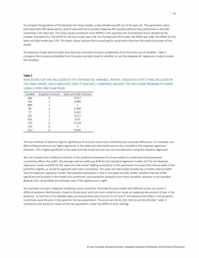
Table 4 THE PRIOR MEANS AND VARIANCES FOR EACH OF THE UNKNOWN COEFFICIENTS IN THE REGRESSION MODEL. THE DISTRIBUTION OF EACH OF THE PRIORS IS NORMAL.
Variable Prior Mean Prior Variance Age 0 4 Sex −0.5 1 BMI 1 1 BP 1 1 TC 1 1 LDL −1 1 HDL −1 1 TCH 0 4 LTG 0.5 1 GLU 1 1
Everything Else 0 9
The priors for the spike and slab model are defined hierarchically as in Section 3.1.3, with 𝑉𝑉𝜎𝜎 = 𝑏𝑏𝜎𝜎 = 𝑉𝑉𝜏𝜏 = 𝑏𝑏𝜏𝜏 = 0.01. These are noninformative priors, which means that we use very little prior information for the variance terms. The spike term is set to 𝑣𝑣0 =0.005, which was determined by exploring several options and comparing the resulting fit.
25
© 2017 Casualty Actuarial Society, Canadian Institute of Actuaries, and Society of Actuaries
To compare the goodness of fits between the three models, a test sample was left out of the data set. The parameters were estimated with 400 observations, and 42 were left out to predict (stepwise AIC variable selection was performed on the 400 remaining in the data set). The mean square prediction error (MSPE) is the squared sum of prediction errors divided by the number of predictions. The MSPE for the OLS model was 4.28. For the Bayesian OLS model, the MSPE was 3.88. The MSPE for the spike and slab model was 3.50. The lower values indicate that accounting for uncertainty improves the predictive power of the model.
The Bayesian model with the spike and slab prior estimates inclusion probabilities from the entire set of variables. Table 5 compares the inclusion probability from the spike and slab model to whether or not the stepwise AIC regression model includes the variables.
Table 5 INDICATORS FOR THE INCLUSION IN THE STEPWISE AIC VARIABLE, WHERE 1 INDICATES THAT IT WAS INCLUDED IN THE FINAL MODEL AND 0 INDICATES THAT IT WAS NOT, COMPARED AGAINST THE INCLUSION PROBABILITY WHEN USING A SPIKE AND SLAB PRIOR.
Variable Stepwise Inclusion Spike and Slab Inclusion Age 0 0.517 Sex 1 0.985 BMI 1 1 BP 1 0.998 TC 1 0.451 LDL 1 0.511 HDL 1 0.97 TCH 0 0.724 LTG 0 1 GLU 0 0.645
The two methods of determining the significance of inclusion have many similarities but some key differences. For example, sex, BMI and blood pressure are highly significant in the spike and slab model and are also included in the stepwise regression. However, LTG is highly significant in the spike and slab model and yet was not included when using the stepwise regression.
We can compare the confidence intervals of the predictions between the three models to understand how parameter uncertainty affects the width. The average interval width was 8.84 for the standard regression model, 9.07 for the Bayesian regression model and 8.90 for the spike and slab model. Adding uncertainty in the parameters increases the interval width of the prediction slightly, as would be expected with extra uncertainty. The spike and slab model actually has a smaller interval width than the Bayesian regression model. One possible explanation is that in the spike and slab model, variables that are mildly significant are included in the model only sometimes, decreasing the variability from these variables, whereas in the standard Bayesian OLS, all variables are included, even if the significance is slight.
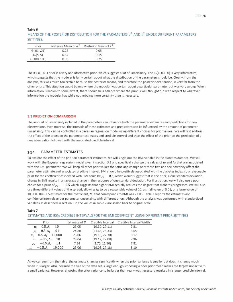
An important concept in Bayesian modeling is prior sensitivity. Running the same model with different priors can result in different posterior distributions. A poorly chosen prior with too much certainty can cause an inappropriate amount of bias in the posterior. To test this in the diabetes data, we choose three sets of priors for 𝜎𝜎2 and 𝜏𝜏2 and examine the effect in the posterior. In all three cases the prior is the same for the two parameters. The priors are IG(.01,.01), IG(5,5) and IG(100,100). Table 6 summarizes the posterior means of the two parameters under the different prior settings.
26
© 2017 Casualty Actuarial Society, Canadian Institute of Actuaries, and Society of Actuaries
Table 6 MEANS OF THE POSTERIOR DISTRIBUTION FOR THE PARAMETERS 𝜎𝜎2 AND 𝜏𝜏2 UNDER DIFFERENT PARAMETERS SETTINGS.
Prior Posterior Mean of 𝜎𝜎2 Posterior Mean of 𝜏𝜏2 IG(.01, .01) 0.25 0.05
IG(5, 5) 0.37 0.15 IG(100, 100) 0.93 0.75
The IG(.01,.01) prior is a very noninformative prior, which suggests a lot of uncertainty. The IG(100,100) is very informative, which suggests that the modeler is fairly certain about what the distribution of the parameters should be. Clearly, from the analysis, this was much too certain because the posterior means, and therefore the posterior distribution, is very far from the other priors. This situation would be one where the modeler was certain about a particular parameter but was very wrong. When information is known to some extent, there should be a balance where the prior is well thought out with respect to whatever information the modeler has while not imbuing more certainty than is necessary.
3.3 PREDICTION COMPARISON The amount of uncertainty included in the parameters can influence both the parameter estimates and predictions for new observations. Even more so, the intervals of these estimates and predictions can be influenced by the amount of parameter uncertainty. This can be controlled in a Bayesian regression model using different choices for prior values. We will first address the effect of the priors on the parameter estimates and credible interval and then the effect of the prior on the prediction of a new observation followed with the associated credible interval.
3.3.1 PARAMETER ESTIMATES
To explore the effect of the prior on parameter estimates, we will single out the BMI variable in the diabetes data set. We will work with the Bayesian regression model given in section 3.1 and specifically change the values of 𝜇𝜇𝑖𝑖 and Λ𝑖𝑖 that are associated with the BMI parameter. We will keep all other prior values the same and change only these two and see how they affect the parameter estimate and associated credible interval. BMI should be positively associated with the diabetes index, so a reasonable prior for the coefficient associated with BMI could be 𝜇𝜇𝑖𝑖 = 0.5, which would suggest that in the prior, a one standard deviation change in BMI results in an average change in the response of one standard deviation. For illustration, we will also use a poor choice for a prior of 𝜇𝜇𝑖𝑖 = −0.5 which suggests that higher BMI actually reduces the degree that diabetes progresses. We will also use three different values of the spread, allowing Λ𝑖𝑖 to be a reasonable value of 10, a small value of 0.01, or a large value of 10,000. The OLS estimate for the coefficient, 𝛽𝛽𝑖𝑖 , that corresponds to BMI was 23.06. Table 7 reports the estimates and confidence intervals under parameter uncertainty with different priors. Although the analysis was performed with standardized variables as described in section 3.2, the values in Table 7 are scaled back to original scale.
Table 7 ESTIMATES AND 95% CREDIBLE INTERVALS FOR THE BMI COEFFICENT USING DIFFERENT PRIOR SETTINGS
Prior Estimate of 𝛽𝛽𝑖𝑖 Credible Interval Credible Interval Width 𝜇𝜇𝑖𝑖 = 0.5,Λ𝑖𝑖 = 10 23.05 (19.30, 27.11) 7.81 𝜇𝜇𝑖𝑖 = 0.5,Λ𝑖𝑖 = .01 24.88 (21.68, 28.33) 6.65
𝜇𝜇𝑖𝑖 = 0.5,Λ𝑖𝑖 = 10,000 23.06 (19.18, 27.30) 8.12 𝜇𝜇𝑖𝑖 = −0.5,Λ𝑖𝑖 = 10 23.04 (19.12, 27.08) 7.96 𝜇𝜇𝑖𝑖 = −0.5,Λ𝑖𝑖 = .01 7.54 (3.70, 11.50) 7.81
𝜇𝜇𝑖𝑖 = −0.5,Λ𝑖𝑖 = 10,000 23.06 (19.08, 27.18) 8.10
As we can see from the table, the estimate changes significantly when the prior variance is smaller but doesn’t change much when it is larger. Also, because the size of the data set is large enough, choosing a poor prior mean makes the largest impact with a small variance. However, choosing the prior variance to be larger than really was necessary resulted in a larger credible interval.
27
© 2017 Casualty Actuarial Society, Canadian Institute of Actuaries, and Society of Actuaries
If tighter intervals are important, it is best to strike a balance in the prior variance and not choose one that is too small so that the prior mean carries too much weight or too large, unnecessarily putting extra uncertainty into the model.
3.3.2 PREDICTIONS OF NEW OBSERVATIONS
We can repeat this study for predictions of new observations. The prior values of 𝑉𝑉 and 𝑏𝑏 play an important role in determining the estimates and intervals of the predictions of new observations. To be clear, the prior expected value of the variance of
observations is 𝑏𝑏𝑎𝑎−1
, so as 𝑏𝑏 increases relative to 𝑉𝑉, the prior variance of the observations increases, and the prediction interval
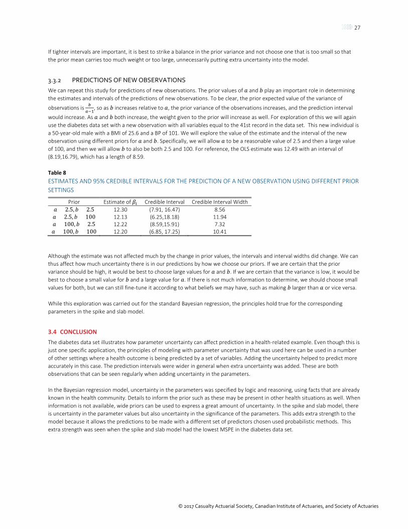
would increase. As 𝑉𝑉 and 𝑏𝑏 both increase, the weight given to the prior will increase as well. For exploration of this we will again use the diabetes data set with a new observation with all variables equal to the 41st record in the data set. This new individual is a 50-year-old male with a BMI of 25.6 and a BP of 101. We will explore the value of the estimate and the interval of the new observation using different priors for 𝑉𝑉 and 𝑏𝑏. Specifically, we will allow 𝑉𝑉 to be a reasonable value of 2.5 and then a large value of 100, and then we will allow 𝑏𝑏 to also be both 2.5 and 100. For reference, the OLS estimate was 12.49 with an interval of (8.19,16.79), which has a length of 8.59.
Table 8 ESTIMATES AND 95% CREDIBLE INTERVALS FOR THE PREDICTION OF A NEW OBSERVATION USING DIFFERENT PRIOR SETTINGS
Prior Estimate of 𝛽𝛽𝑖𝑖 Credible Interval Credible Interval Width 𝑉𝑉 = 2.5,𝑏𝑏 = 2.5 12.30 (7.91, 16.47) 8.56 𝑉𝑉 = 2.5, 𝑏𝑏 = 100 12.13 (6.25,18.18) 11.94 𝑉𝑉 = 100,𝑏𝑏 = 2.5 12.22 (8.59,15.91) 7.32 𝑉𝑉 = 100,𝑏𝑏 = 100 12.20 (6.85, 17.25) 10.41
Although the estimate was not affected much by the change in prior values, the intervals and interval widths did change. We can thus affect how much uncertainty there is in our predictions by how we choose our priors. If we are certain that the prior variance should be high, it would be best to choose large values for 𝑉𝑉 and 𝑏𝑏. If we are certain that the variance is low, it would be best to choose a small value for 𝑏𝑏 and a large value for 𝑉𝑉. If there is not much information to determine, we should choose small values for both, but we can still fine-tune it according to what beliefs we may have, such as making 𝑏𝑏 larger than 𝑉𝑉 or vice versa.
While this exploration was carried out for the standard Bayesian regression, the principles hold true for the corresponding parameters in the spike and slab model.
3.4 CONCLUSION The diabetes data set illustrates how parameter uncertainty can affect prediction in a health-related example. Even though this is just one specific application, the principles of modeling with parameter uncertainty that was used here can be used in a number of other settings where a health outcome is being predicted by a set of variables. Adding the uncertainty helped to predict more accurately in this case. The prediction intervals were wider in general when extra uncertainty was added. These are both observations that can be seen regularly when adding uncertainty in the parameters.
In the Bayesian regression model, uncertainty in the parameters was specified by logic and reasoning, using facts that are already known in the health community. Details to inform the prior such as these may be present in other health situations as well. When information is not available, wide priors can be used to express a great amount of uncertainty. In the spike and slab model, there is uncertainty in the parameter values but also uncertainty in the significance of the parameters. This adds extra strength to the model because it allows the predictions to be made with a different set of predictors chosen used probabilistic methods. This extra strength was seen when the spike and slab model had the lowest MSPE in the diabetes data set.
28
© 2017 Casualty Actuarial Society, Canadian Institute of Actuaries, and Society of Actuaries
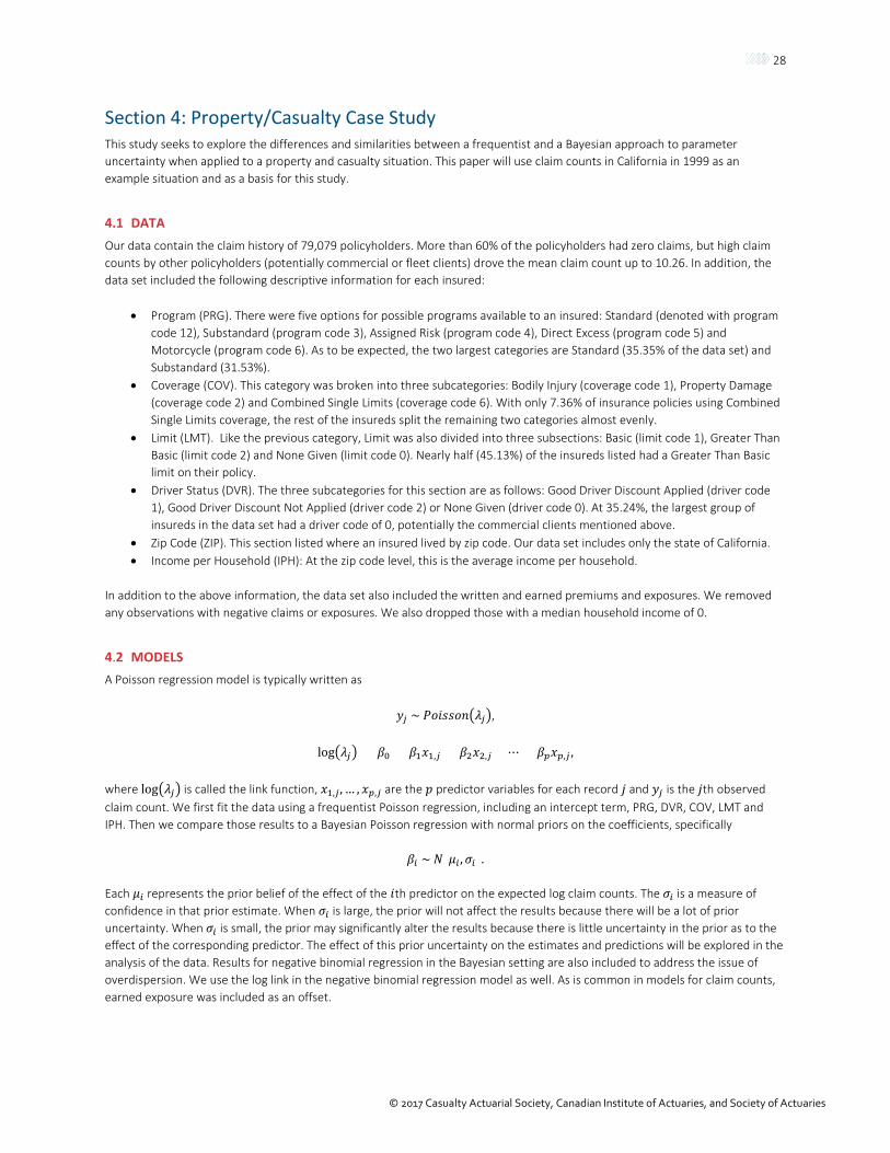
Section 4: Property/Casualty Case Study This study seeks to explore the differences and similarities between a frequentist and a Bayesian approach to parameter uncertainty when applied to a property and casualty situation. This paper will use claim counts in California in 1999 as an example situation and as a basis for this study.
4.1 DATA Our data contain the claim history of 79,079 policyholders. More than 60% of the policyholders had zero claims, but high claim counts by other policyholders (potentially commercial or fleet clients) drove the mean claim count up to 10.26. In addition, the data set included the following descriptive information for each insured:
• Program (PRG). There were five options for possible programs available to an insured: Standard (denoted with programcode 12), Substandard (program code 3), Assigned Risk (program code 4), Direct Excess (program code 5) andMotorcycle (program code 6). As to be expected, the two largest categories are Standard (35.35% of the data set) andSubstandard (31.53%).
• Coverage (COV). This category was broken into three subcategories: Bodily Injury (coverage code 1), Property Damage(coverage code 2) and Combined Single Limits (coverage code 6). With only 7.36% of insurance policies using CombinedSingle Limits coverage, the rest of the insureds split the remaining two categories almost evenly.
• Limit (LMT). Like the previous category, Limit was also divided into three subsections: Basic (limit code 1), Greater ThanBasic (limit code 2) and None Given (limit code 0). Nearly half (45.13%) of the insureds listed had a Greater Than Basiclimit on their policy.
• Driver Status (DVR). The three subcategories for this section are as follows: Good Driver Discount Applied (driver code1), Good Driver Discount Not Applied (driver code 2) or None Given (driver code 0). At 35.24%, the largest group of insureds in the data set had a driver code of 0, potentially the commercial clients mentioned above.
• Zip Code (ZIP). This section listed where an insured lived by zip code. Our data set includes only the state of California. • Income per Household (IPH): At the zip code level, this is the average income per household.
In addition to the above information, the data set also included the written and earned premiums and exposures. We removed any observations with negative claims or exposures. We also dropped those with a median household income of 0.
4.2 MODELS A Poisson regression model is typically written as
𝑦𝑦𝑗𝑗 ~ 𝑃𝑃𝑃𝑃𝑃𝑃𝑃𝑃𝑃𝑃𝑃𝑃𝐵𝐵�𝜆𝜆𝑗𝑗�,
log�𝜆𝜆𝑗𝑗� = 𝛽𝛽0 + 𝛽𝛽1𝑥𝑥1,𝑗𝑗 + 𝛽𝛽2𝑥𝑥2,𝑗𝑗 + ⋯+ 𝛽𝛽𝑝𝑝𝑥𝑥𝑝𝑝,𝑗𝑗 ,
where log�𝜆𝜆𝑗𝑗� is called the link function, 𝑥𝑥1,𝑗𝑗 , … , 𝑥𝑥𝑝𝑝,𝑗𝑗 are the 𝑝𝑝 predictor variables for each record 𝑗𝑗 and 𝑦𝑦𝑗𝑗 is the 𝑗𝑗th observed claim count. We first fit the data using a frequentist Poisson regression, including an intercept term, PRG, DVR, COV, LMT and IPH. Then we compare those results to a Bayesian Poisson regression with normal priors on the coefficients, specifically
𝛽𝛽𝑖𝑖 ~ 𝑁𝑁(𝜇𝜇𝑖𝑖 ,𝜎𝜎𝑖𝑖).
Each 𝜇𝜇𝑖𝑖 represents the prior belief of the effect of the 𝑃𝑃th predictor on the expected log claim counts. The 𝜎𝜎𝑖𝑖 is a measure of confidence in that prior estimate. When 𝜎𝜎𝑖𝑖 is large, the prior will not affect the results because there will be a lot of prior uncertainty. When 𝜎𝜎𝑖𝑖 is small, the prior may significantly alter the results because there is little uncertainty in the prior as to the effect of the corresponding predictor. The effect of this prior uncertainty on the estimates and predictions will be explored in the analysis of the data. Results for negative binomial regression in the Bayesian setting are also included to address the issue of overdispersion. We use the log link in the negative binomial regression model as well. As is common in models for claim counts, earned exposure was included as an offset.
29
© 2017 Casualty Actuarial Society, Canadian Institute of Actuaries, and Society of Actuaries
4.3 RESULTS
4.3.1 POISSON REGRESSION
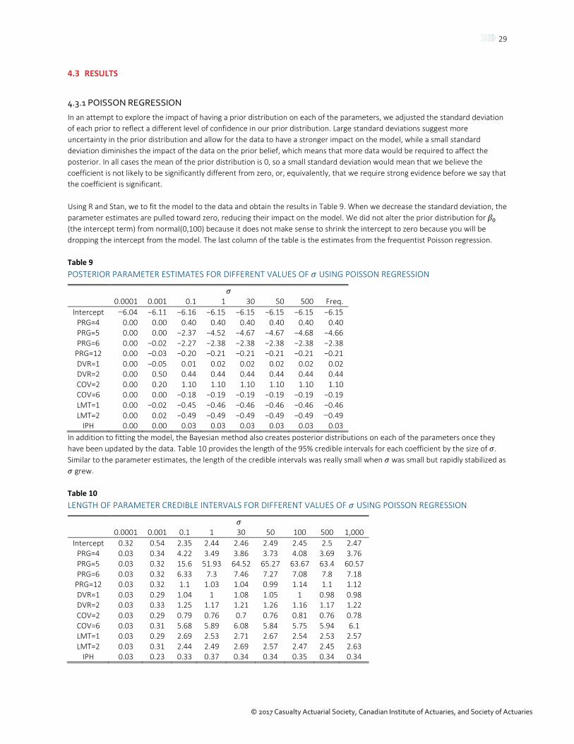
In an attempt to explore the impact of having a prior distribution on each of the parameters, we adjusted the standard deviation of each prior to reflect a different level of confidence in our prior distribution. Large standard deviations suggest more uncertainty in the prior distribution and allow for the data to have a stronger impact on the model, while a small standard deviation diminishes the impact of the data on the prior belief, which means that more data would be required to affect the posterior. In all cases the mean of the prior distribution is 0, so a small standard deviation would mean that we believe the coefficient is not likely to be significantly different from zero, or, equivalently, that we require strong evidence before we say that the coefficient is significant.
Using R and Stan, we to fit the model to the data and obtain the results in Table 9. When we decrease the standard deviation, the parameter estimates are pulled toward zero, reducing their impact on the model. We did not alter the prior distribution for 𝛽𝛽0 (the intercept term) from normal(0,100) because it does not make sense to shrink the intercept to zero because you will be dropping the intercept from the model. The last column of the table is the estimates from the frequentist Poisson regression.
Table 9 POSTERIOR PARAMETER ESTIMATES FOR DIFFERENT VALUES OF 𝜎𝜎 USING POISSON REGRESSION
𝜎𝜎 0.0001 0.001 0.1 1 30 50 500 Freq.
Intercept −6.04 −6.11 −6.16 −6.15 −6.15 −6.15 −6.15 −6.15 PRG=4 0.00 0.00 0.40 0.40 0.40 0.40 0.40 0.40 PRG=5 0.00 0.00 −2.37 −4.52 −4.67 −4.67 −4.68 −4.66 PRG=6 0.00 −0.02 −2.27 −2.38 −2.38 −2.38 −2.38 −2.38
PRG=12 0.00 −0.03 −0.20 −0.21 −0.21 −0.21 −0.21 −0.21 DVR=1 0.00 −0.05 0.01 0.02 0.02 0.02 0.02 0.02 DVR=2 0.00 0.50 0.44 0.44 0.44 0.44 0.44 0.44 COV=2 0.00 0.20 1.10 1.10 1.10 1.10 1.10 1.10 COV=6 0.00 0.00 −0.18 −0.19 −0.19 −0.19 −0.19 −0.19 LMT=1 0.00 −0.02 −0.45 −0.46 −0.46 −0.46 −0.46 −0.46 LMT=2 0.00 0.02 −0.49 −0.49 −0.49 −0.49 −0.49 −0.49
IPH 0.00 0.00 0.03 0.03 0.03 0.03 0.03 0.03 In addition to fitting the model, the Bayesian method also creates posterior distributions on each of the parameters once they have been updated by the data. Table 10 provides the length of the 95% credible intervals for each coefficient by the size of 𝜎𝜎. Similar to the parameter estimates, the length of the credible intervals was really small when 𝜎𝜎 was small but rapidly stabilized as 𝜎𝜎 grew.
Table 10 LENGTH OF PARAMETER CREDIBLE INTERVALS FOR DIFFERENT VALUES OF 𝜎𝜎 USING POISSON REGRESSION
𝜎𝜎 0.0001 0.001 0.1 1 30 50 100 500 1,000
Intercept 0.32 0.54 2.35 2.44 2.46 2.49 2.45 2.5 2.47 PRG=4 0.03 0.34 4.22 3.49 3.86 3.73 4.08 3.69 3.76 PRG=5 0.03 0.32 15.6 51.93 64.52 65.27 63.67 63.4 60.57 PRG=6 0.03 0.32 6.33 7.3 7.46 7.27 7.08 7.8 7.18
PRG=12 0.03 0.32 1.1 1.03 1.04 0.99 1.14 1.1 1.12 DVR=1 0.03 0.29 1.04 1 1.08 1.05 1 0.98 0.98 DVR=2 0.03 0.33 1.25 1.17 1.21 1.26 1.16 1.17 1.22 COV=2 0.03 0.29 0.79 0.76 0.7 0.76 0.81 0.76 0.78 COV=6 0.03 0.31 5.68 5.89 6.08 5.84 5.75 5.94 6.1 LMT=1 0.03 0.29 2.69 2.53 2.71 2.67 2.54 2.53 2.57 LMT=2 0.03 0.31 2.44 2.49 2.69 2.57 2.47 2.45 2.63
IPH 0.03 0.23 0.33 0.37 0.34 0.34 0.35 0.34 0.34
30
© 2017 Casualty Actuarial Society, Canadian Institute of Actuaries, and Society of Actuaries
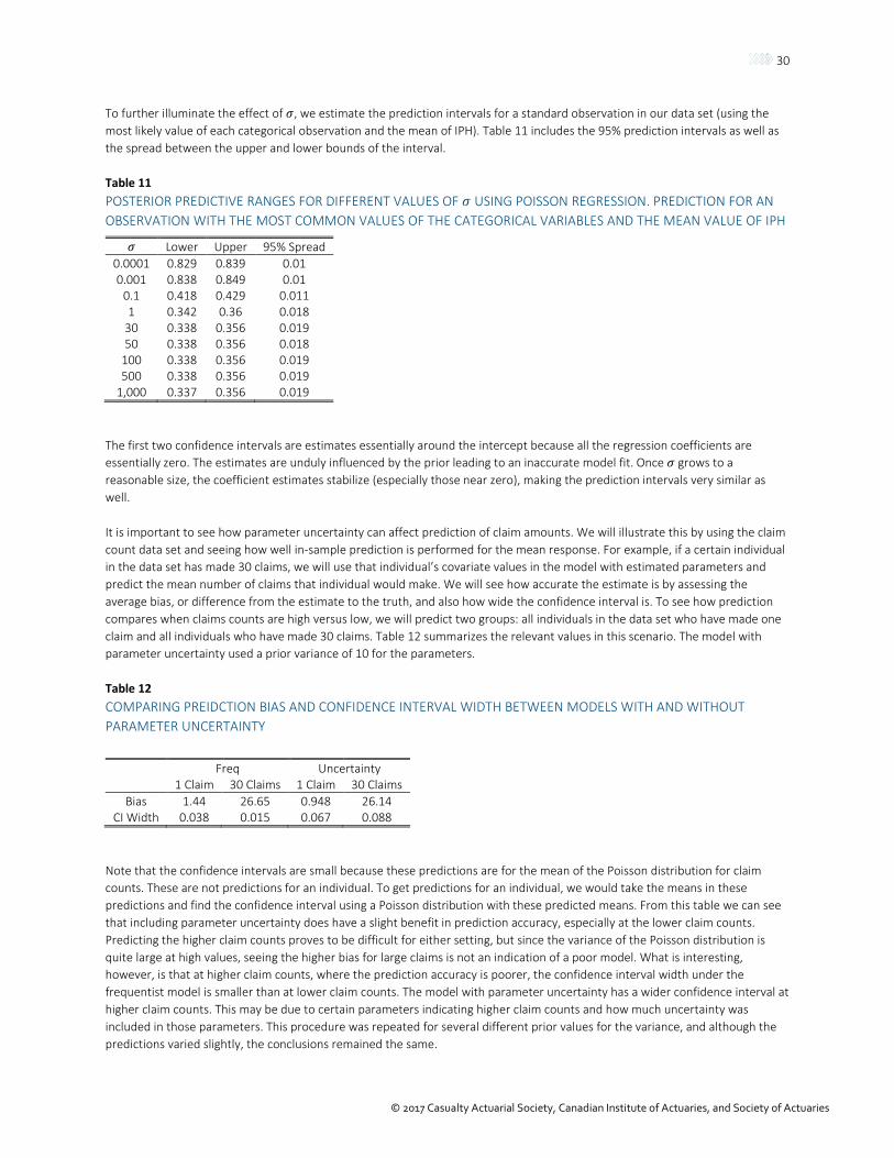
To further illuminate the effect of 𝜎𝜎, we estimate the prediction intervals for a standard observation in our data set (using the most likely value of each categorical observation and the mean of IPH). Table 11 includes the 95% prediction intervals as well as the spread between the upper and lower bounds of the interval.
Table 11 POSTERIOR PREDICTIVE RANGES FOR DIFFERENT VALUES OF 𝜎𝜎 USING POISSON REGRESSION. PREDICTION FOR AN OBSERVATION WITH THE MOST COMMON VALUES OF THE CATEGORICAL VARIABLES AND THE MEAN VALUE OF IPH
𝜎𝜎 Lower Upper 95% Spread 0.0001 0.829 0.839 0.01 0.001 0.838 0.849 0.01
0.1 0.418 0.429 0.011 1 0.342 0.36 0.018
30 0.338 0.356 0.019 50 0.338 0.356 0.018
100 0.338 0.356 0.019 500 0.338 0.356 0.019
1,000 0.337 0.356 0.019
The first two confidence intervals are estimates essentially around the intercept because all the regression coefficients are essentially zero. The estimates are unduly influenced by the prior leading to an inaccurate model fit. Once 𝜎𝜎 grows to a reasonable size, the coefficient estimates stabilize (especially those near zero), making the prediction intervals very similar as well.
It is important to see how parameter uncertainty can affect prediction of claim amounts. We will illustrate this by using the claim count data set and seeing how well in-sample prediction is performed for the mean response. For example, if a certain individual in the data set has made 30 claims, we will use that individual’s covariate values in the model with estimated parameters and predict the mean number of claims that individual would make. We will see how accurate the estimate is by assessing the average bias, or difference from the estimate to the truth, and also how wide the confidence interval is. To see how prediction compares when claims counts are high versus low, we will predict two groups: all individuals in the data set who have made one claim and all individuals who have made 30 claims. Table 12 summarizes the relevant values in this scenario. The model with parameter uncertainty used a prior variance of 10 for the parameters.
Table 12 COMPARING PREIDCTION BIAS AND CONFIDENCE INTERVAL WIDTH BETWEEN MODELS WITH AND WITHOUT PARAMETER UNCERTAINTY
Freq Uncertainty 1 Claim 30 Claims 1 Claim 30 Claims
Bias 1.44 26.65 0.948 26.14 CI Width 0.038 0.015 0.067 0.088
Note that the confidence intervals are small because these predictions are for the mean of the Poisson distribution for claim counts. These are not predictions for an individual. To get predictions for an individual, we would take the means in these predictions and find the confidence interval using a Poisson distribution with these predicted means. From this table we can see that including parameter uncertainty does have a slight benefit in prediction accuracy, especially at the lower claim counts. Predicting the higher claim counts proves to be difficult for either setting, but since the variance of the Poisson distribution is quite large at high values, seeing the higher bias for large claims is not an indication of a poor model. What is interesting, however, is that at higher claim counts, where the prediction accuracy is poorer, the confidence interval width under the frequentist model is smaller than at lower claim counts. The model with parameter uncertainty has a wider confidence interval at higher claim counts. This may be due to certain parameters indicating higher claim counts and how much uncertainty was included in those parameters. This procedure was repeated for several different prior values for the variance, and although the predictions varied slightly, the conclusions remained the same.
31
© 2017 Casualty Actuarial Society, Canadian Institute of Actuaries, and Society of Actuaries
4.3.2 NEGATIVE BINOMIAL REGRESSION
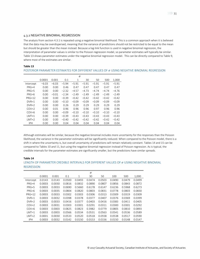
The analysis from section 4.3.1 is repeated using a negative binomial likelihood. This is a common approach when it is believed that the data may be overdispersed, meaning that the variance of predictions should not be restricted to be equal to the mean but should be greater than the mean instead. Because a log-link function is used in negative binomial regression, the interpretation of parameter values is similar to the Poisson regression model, so parameter estimates will typically be similar. Table 13 shows parameter estimates under the negative binomial regression model. This can be directly compared to Table 9, where most of the estimates are similar.
Table 13 POSTERIOR PARAMETER ESTIMATES FOR DIFFERENT VALUES OF 𝜎𝜎 USING NEGATIVE BINOMIAL REGRESSION
𝜎𝜎 0.0001 0.001 0.1 1 30 50 500 1,000
Intercept −6.03 −6.03 −5.94 −5.91 −5.91 −5.91 −5.91 −5.91 PRG=4 0.00 0.00 0.46 0.47 0.47 0.47 0.47 0.47 PRG=5 0.00 0.00 −2.32 −4.57 −4.73 −4.74 −4.74 −4.76 PRG=6 0.00 −0.01 −2.34 −2.49 −2.49 −2.49 −2.49 −2.49
PRG=12 0.00 0.00 −0.39 −0.42 −0.42 −0.42 −0.42 −0.42 DVR=1 0.00 0.00 −0.10 −0.09 −0.09 −0.09 −0.09 −0.09 DVR=2 0.00 0.00 0.26 0.29 0.29 0.29 0.29 0.29 COV=2 0.00 0.01 0.96 0.96 0.96 0.97 0.96 0.96 COV=6 0.00 0.00 −0.09 −0.10 −0.10 −0.10 −0.10 −0.10 LMT=1 0.00 0.00 −0.39 −0.43 −0.43 −0.43 −0.43 −0.43 LMT=2 0.00 0.00 −0.40 −0.42 −0.42 −0.42 −0.42 −0.42
IPH 0.00 0.00 0.04 0.04 0.04 0.04 0.04 0.04
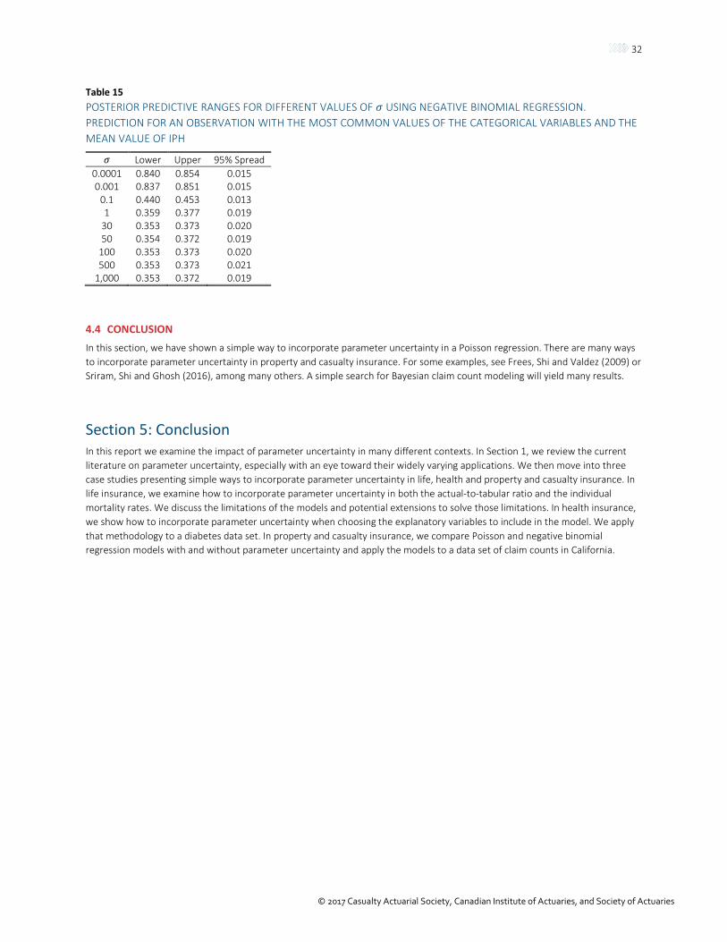
Although estimates will be similar, because the negative binomial includes more uncertainty for the responses than the Poisson likelihood, the variance in the parameter estimates will be significantly reduced. When compared to the Poisson model, there is a shift in where the uncertainty is, but overall uncertainty of predictions will remain relatively constant. Tables 14 and 15 can be compared to Tables 10 and 11, but using the negative binomial regression instead of Poisson regression. As is typical, the credible intervals for the parameter estimates are significantly smaller, but the predictions have similar spreads.
Table 14 LENGTH OF PARAMETER CREDIBLE INTERVALS FOR DIFFERENT VALUES OF 𝜎𝜎 USING NEGATIVE BINOMIAL REGRESSION
𝜎𝜎 0.0001 0.001 0.1 1 30 50 100 500 1,000
Intercept 0.0143 0.0143 0.0500 0.0493 0.0474 0.0503 0.0490 0.0479 0.0499 PRG=4 0.0003 0.0030 0.0816 0.0832 0.0890 0.0807 0.0856 0.0843 0.0872 PRG=5 0.0003 0.0033 0.0690 0.5660 0.6178 0.6147 0.6236 0.5968 0.6273 PRG=6 0.0003 0.0035 0.0804 0.0820 0.0803 0.0831 0.0778 0.0803 0.0830
PRG=12 0.0003 0.0033 0.0302 0.0303 0.0306 0.0313 0.0309 0.0319 0.0309 DVR=1 0.0003 0.0032 0.0398 0.0378 0.0377 0.0407 0.0376 0.0369 0.0399 DVR=2 0.0003 0.0033 0.0416 0.0377 0.0403 0.0416 0.0383 0.0411 0.0405 COV=2 0.0003 0.0031 0.0303 0.0301 0.0291 0.0311 0.0300 0.0301 0.0292 COV=6 0.0003 0.0003 0.0825 0.0823 0.3982 0.0779 0.0805 0.0810 0.0893 LMT=1 0.0003 0.0003 0.0566 0.0534 0.0531 0.0563 0.0541 0.0536 0.0589 LMT=2 0.0001 0.0030 0.0533 0.0520 0.0518 0.0558 0.0538 0.0517 0.0590
IPH 0.0003 0.0032 0.0142 0.0150 0.0153 0.0156 0.0150 0.0148 0.0147
32
© 2017 Casualty Actuarial Society, Canadian Institute of Actuaries, and Society of Actuaries
Table 15 POSTERIOR PREDICTIVE RANGES FOR DIFFERENT VALUES OF 𝜎𝜎 USING NEGATIVE BINOMIAL REGRESSION. PREDICTION FOR AN OBSERVATION WITH THE MOST COMMON VALUES OF THE CATEGORICAL VARIABLES AND THE MEAN VALUE OF IPH
𝜎𝜎 Lower Upper 95% Spread 0.0001 0.840 0.854 0.015 0.001 0.837 0.851 0.015
0.1 0.440 0.453 0.013 1 0.359 0.377 0.019
30 0.353 0.373 0.020 50 0.354 0.372 0.019
100 0.353 0.373 0.020 500 0.353 0.373 0.021
1,000 0.353 0.372 0.019
4.4 CONCLUSION In this section, we have shown a simple way to incorporate parameter uncertainty in a Poisson regression. There are many ways to incorporate parameter uncertainty in property and casualty insurance. For some examples, see Frees, Shi and Valdez (2009) or Sriram, Shi and Ghosh (2016), among many others. A simple search for Bayesian claim count modeling will yield many results.
Section 5: Conclusion In this report we examine the impact of parameter uncertainty in many different contexts. In Section 1, we review the current literature on parameter uncertainty, especially with an eye toward their widely varying applications. We then move into three case studies presenting simple ways to incorporate parameter uncertainty in life, health and property and casualty insurance. In life insurance, we examine how to incorporate parameter uncertainty in both the actual-to-tabular ratio and the individual mortality rates. We discuss the limitations of the models and potential extensions to solve those limitations. In health insurance, we show how to incorporate parameter uncertainty when choosing the explanatory variables to include in the model. We apply that methodology to a diabetes data set. In property and casualty insurance, we compare Poisson and negative binomial regression models with and without parameter uncertainty and apply the models to a data set of claim counts in California.
33
© 2017 Casualty Actuarial Society, Canadian Institute of Actuaries, and Society of Actuaries
Section 6: References Beck, J. L., & Katafygiotis, L. S. (1998). Updating models and their uncertainties. I: Bayesian statistical framework. Journal of Engineering Mechanics, 124, 455–461. Bignozzi, V., & Tsanakas, A. (2015). Parameter uncertainty and residual estimation risk. Journal of Risk and Insurance, 83(4), 949-978, 2016.
Borowicz, J. M., & Norman, J. P. (2006). The effects of parameter uncertainty in the extreme event frequency-severity model. 28th International Congress of Actuaries, 28. Paris.
Cairns, A. J. (2000). A discussion of parameter and model uncertainty in insurance. Insurance: Mathematics and Economics, 124, 313–330.
Cairns, A. J., Blake, D., & Dowd, K. (2006). A two-factor model for stochastic mortality with parameter uncertainty: Theory and calibration. Journal of Risk and Insurance, 73, 687–718.
Diers, D., Eling, M., & Linde, M. (2013). Modeling parameter risk in premium risk in multi-year internal models. Journal of Risk Finance, 14, 234–250.
Efron, B., Hastie, T., Johnstone, I., & Tibshirani, R. (2004). Least angle regression (with discussion). Annals of Statistics, 32, 407–499.
Fellingham, G. W., Kottas, A., & Hartman, B. M. (2015). Bayesian nonparametric predictive modeling of group health claims. Insurance: Mathematics and Economics, 60, 1–10.
Frees, E. W., Shi, P., & Valdez, E. A. (2009). Actuarial applications of a hierarchical insurance claims model. ASTIN Bulletin, 39, 165–197.
Gelman, A., Carlin, J. B., Stern, H. S., & Rubin, D. B. (2014). Bayesian data analysis (Vol. 2). Boca Raton, FL: Chapman & Hall.
Gerrard, R., & Tsanakas, A. (2011). Failure probability under parameter uncertainty. Risk Analysis, 31, 727–744.
Hartman, B. M., & Groendyke, C. (2013). Model selection and averaging in financial risk management. North American Actuarial Journal, 17, 216–228.
Hartman, B. M., & Heaton, M. J. (2011). Accounting for regime and parameter uncertainty in regime-switching models. Insurance: Mathematics and Economics, 49, 429–437.
Hayne, R. M. (1999). Modeling parameter uncertainty in cash flow projections. Casualty Actuarial Society Forum, 133–151.
Heckman, P. E., & Meyers, G. G. (1983). The calculation of aggregate loss distributions from claim severity and claim count distributions. Proceedings of the Casualty Actuarial Society, 70, 22–61.
Ishwaran, H., & Rao, J. S. (2005). Spike and slab variable selection: Frequentist and Bayesian strategies. Annals of Statistics, 33, 730–773.
Kitanidis, P. K. (1986). Parameter uncertainty in estimation of spatial functions: Bayesian analysis. Water Resources Research, 22, 499–507.
Marin, J. M., & Robert, C. (2007). Bayesian core: A practical approach to computational Bayesian statistics. Springer Science & Business Media.
Meyers, G. (1999). Estimating between line correlations generated by parameter uncertainty. Casualty Actuarial Society Forum, 197.
Meyers, G., & Schenker, N. (1983). Parameter uncertainty in the collective risk model. Proceedings of the Casualty Actuarial Society, 70, 111.
Meyers, G. G. (2007). Estimating predictive distributions for loss reserve models. Variance, 1, 248–272.
Shi, P., Basu, S., & Meyers, G. G. (2012). A Bayesian log-normal model for multivariate loss reserving. North American Actuarial Journal, 16, 29–51.
Shi, P., & Hartman, B. M. (2016). Credibility in loss reserving. North American Actuarial Journal, 20(2), 114–132.

34
© 2017 Casualty Actuarial Society, Canadian Institute of Actuaries, and Society of Actuaries
Smith, R. C. (2013). Uncertainty quantification: Theory, implementation, and applications (Vol. 12). SIAM, Philadelphia.
Sriram, K., Shi, P., & Ghosh, P. (2016). A Bayesian quantile regression model for insurance company costs data. Journal of the Royal Statistical Society: Series A (Statistics in Society), 179, 177–202.
Venter, G. G., & Sahasrabuddhe, R. V. (2015). A note on parameter risk. Variance, 9, 54–63.
Wacek, M. G. (2005). Parameter uncertainty in loss ratio distributions and its implications. Casualty Actuarial Society Forum, 3, 165–202.
Wood, E. F., & Rodriguez-Iturbe, I. (1975). Bayesian inference and decision making for extreme hydrologic events. Water Resources Research, 11, 533–542.
Recommended