ORIGINAL PAPER - PRODUCTION ENGINEERING

Quantifying uncertainty in infill well placement using numericalsimulation and experimental design: case study

Akeem O. Arinkoola1 • Haruna M. Onuh1 • David O. Ogbe1,2

Received: 16 September 2014 / Accepted: 17 May 2015 / Published online: 7 June 2015

� The Author(s) 2015. This article is published with open access at Springerlink.com

Abstract The risky nature of petroleum exploration and

production requires that the decisions on reservoir man-

agement must consider uncertainties and risks associated

with all proposed development programmes. The primary

objective of the case study was to evaluate infill drilling

potentials. However, the selection of type and placement of

the proposed infill wells has been a challenge due to the

presence of large number of uncertainty. The study utilized

numerical simulation, pressure, and saturation maps to

determine infill well location and its optimal placement

within the reservoir. Evaluation and selection of infill

opportunity was carried out by simulating reservoir incre-

mental oil production and water breakthrough time from

vertical and horizontal wells completed within the reservoir

sub-regions. For proxy modeling, Placket–Burman and

uniform design were integrated. Quadratic response surface

was developed and validated. For uncertainty quantifica-

tion, a full Bayesian treatment of uncertainty was per-

formed using Markov Chain Monte Carlo. The posterior

summaries of the parameters along side their uncertainties

given by P2.5 %, P10 %, P50 %, P97.5 %, and P90 %

quartiles were identified for investment decisions. The

methodology is straight forward, easy and can be applied in

other fields for the assessment of infill opportunity

involving infill location, selection, and placement as well

its associated risks for optimal return on investment.

Keywords Sensitivity analysis � Experimental design �Response surface methodology � Proxy model � MCMC �Numerical simulation

Nomenclature

P10 Low case

P50 Base/mid case

P90 High case

M Thousand

MM Million

mD Milidarcy

STB Stock-tank-barrel

MULTFLT Fault transmissibility multiplier

PV Pore volume

FVF Oil formation volume factor

F Field

WCT Water cut

OPT Total oil production

WPT Total water production

GOR Gas–oil ratio

PERMX Horizontal permeability

PERMZ Vertical permeability

WBT Water breakthrough time

SWI Initial water saturation

PORO Porosity

OVISC Oil viscosity

MCS Monte Carlo simulation

& Akeem O. Arinkoola

moranroolaakeem@yahoo.com

Haruna M. Onuh

onuhharuna@yahoo.com

David O. Ogbe

dogreatland@gmail.com

1 Department of Petroleum Engineering, African University of

Science and Technology (AUST), Abuja, Nigeria

2 Flowgrids, Port Harcourt, Nigeria

123

J Petrol Explor Prod Technol (2016) 6:201–215

DOI 10.1007/s13202-015-0180-z

Introduction

The original problem objective of the case study was to

evaluate infill drilling potentials and quantify associated

uncertainty. Permeability and porosity fields are two major

uncertainties identified during the static modeling phase.

Other uncertainties became known after the history matching

phase and fromanalogy using the near-by fields. Therewas no

core information available, and petrophysical properties were

generated using existing correlations. Presently, the reservoir

is producing under primary recovery with recovery factor

approximate 28 %. This recovery is uncharacteristic of Niger

Delta under the current mechanism and it desires to improve

on this factor to about 35 %. Itwas conceived that by reducing

well spacing, reservoir heterogeneity, and layer continuity

can be changed to enhance well connectivity which in turns

can improve oil recovery by accelerating production. How-

ever, due to large uncertainty, infill well performance can

seriously be hampered. Hence, uncertainty quantification

becomes an integral part of this study.

As pointed out by Subbey et al. (2003) and Bustamante

et al. (2005), the success of infill drilling is directly related

to the uncertainties associated with it. Individual reservoir

uncertainties (static and dynamic) all add up to give a

resultant total uncertainty associated in particular, with

performance of infill drilling. There are several methods for

uncertainty estimation. Analytical methods are character-

ized by several assumptions and are becoming less efficient

in estimation and quantification of various uncertainties

due to increasing complexity of petroleum reservoirs.

Some other common methods include Monte Carlo tech-

nique (Hammersley and Handscomb 1964), derivative tree

technique (Steagall and Schiozer 2001), and statistical

theory (Venkataraman 2000). Floris et al. (2001) had pro-

vided comprehensive comparison of the performance, in

terms of accuracy, of some existing methods used for

quantification of uncertainty of production forecasts.

However, detail review on uncertainty estimation and

analysis can be obtained from Amaefule and Keelan (1989)

, Akinwumi et al. (2004), Ballin et al. (2001), and Alhuthali

et al. (2006).

Drilling infill wells, according to Ofoh (1992) can

improve the recovery of hydrocarbon by accelerating the

hydrocarbon productions. However, the determination of

infill potential as well as selection of well type and place-

ment has been a challenge (Thakur and Satter 1998). The

recommended way to determine infill drilling potential in a

reservoir is to conduct a complete reservoir evaluation

involving geological, geophysical, and reservoir analyses

and interpretations. This approach is prohibitively time-

consuming and expensive for some large hydrocarbon fields

(Linhua et al. 2005). Infill Drilling Predictive Model

(IDPM) which requires minimum amount of reservoir and

geologic description has also been used (Fuller et al. 1992).

However, IDPM requires knowledge of heterogeneity ele-

ments (pay continuity and permeability variation among

layers.) which are not easily or often measured in actual

fields. Voneiff and Cipolla (1996) developed a model-based

analysis method, the moving window technique, and apply

it for rapid assessment of infill and re-completion potential

in the Ozona field. The method according to the authors is

quick but the accuracy decreases with increasing hetero-

geneity. Empirical correlations (Hudson et al. 2000) are also

available to determine infill potential in a complex, low-

permeability gas reservoir. These correlations are reservoir

specific and therefore have gained limited applications. The

use of numerical-based instead of analytical-based con-

ceptual models has been reported (Ogbe et al. 2009).

Conceptualized models have been used to provide answers

to frequently asked questions such as the numbers of wells

and their optimum placement within the reservoir. In this

study, a full-field numerical simulation was conducted for

the determination of infill location, infill type selection, and

its placement within the reservoir sub-regions. For accurate

uncertainty quantification, a good proxy is needed. Our

methodology included use of modern experimental design

(UD) to determine the locations of sample points within the

design space instead of conventional designs like central

composite, Box–Behnken, and full factorial designs. Least-

Squares method was used to construct response surface and

to interpolate a limited number of data obtained from sim-

ulation for uncertainty quantification.

Methodology

Grid set-up and model initialization

The top surface map and well location of the case study is

shown in Fig. 1. The reservoir is penetrated by seven wells,

all deviated. The dynamic simulation model was con-

structed using a 100 9 100 9 1 ft believed to preserve

reservoir heterogeneity and accommodate a quick simula-

tion runs. The grid was created using corner point geometry

with dimension of 300 9 300 ft. The reservoir average

porosity is 26.4 %, and average water saturation and per-

meability are 27 % and 700 mD, respectively. The reser-

voir has an initial pressure, Pi = 1950 psia, the API of 22,

FVF of 1.22, and temperature of 165 �F.

Reservoir descriptions of porosity and permeability

The reservoir was divided into four different sub-regions

using faults. In all these regions, permeability ranges from

202 J Petrol Explor Prod Technol (2016) 6:201–215

123

100 to 1300 mD. The vertical variation of permeability

distribution is prevalent in all the regions. The lateral con-

tinuity of permeability was also observed especially in

Regions 1, 2, and 3. For example, the distribution of per-

meability values less than 500 mD in Region 2 is mostly

laterally continuous which is due to presence of stacked beds

with a high degree of lateral continuity. Figure 2 shows

isometric view of the permeability distribution in all the sub-

regions of the reservoir.

The permeability histograms (Fig. 3) of Regions 1 and 3

reflect averages of 500 and 800 mD, respectively. The per-

meability shows amulti-modal distribution inRegions 1with

some small peaks at the extremes of the distribution. These

peaks correspond to shale bodies distributed in the reservoir.

The permeability value was high at the center of the structure

and becomes degraded towards the western direction. In

Region 3, the distribution is fairly normal with mean per-

meability value of 900 mD and standard deviation of 141.4.

Fig. 1 The case study top

surface map and well location

Fig. 2 Isometric view of regional permeability models

J Petrol Explor Prod Technol (2016) 6:201–215 203

123

In Region 4, the permeability is log normal skewed to the

right with mean of 500 mD with some peaks at the extreme

corresponds to shale bodies distributed in the reservoir. In

Region 2, the distribution of permeability is fairly uniform

also with peaks at the lower extreme. The average perme-

ability in this Region ranges between 500 and 720 mD.

Porosity histograms for all the regions are shown in Fig. 4.

Both the porosity and permeability distributions agreed

geologically with high permeability found mostly in high

porosity regions. Generally porosities range between 10 and

27 %. Porosity value as high as 36 % are found in some areas

as well. Porosity distribution in regions 1 and 2 is uniform,

while Regions 3 and 4 exhibited skewed normal distribution.

Pressure and saturation matching

Traditional history matching method (Rwechungura et al.

2011) was adopted. The workflow consists of reservoir type

definition, data preparations/consistency checks, material

balance analysis, pressure and saturation matching, and

results analyses. The material balance tool (MBAL) was

used for the evaluation. The three reservoir drive mecha-

nisms were established to be fluid expansion pore volume

compressibility and water drive. As shown in Fig. 5a, the

predominant energy is water influx. The obtained Analyt-

ical plot in Fig. 5b shows clearly that the observed pro-

duction cannot be matched without the aquifer in place. A

steep drop in reservoir pressure profile when no aquifer

model was included indicates insufficient energy within the

reservoir. The aquifer was modeled numerically and

attached to the grid. Using appropriate aquifer pore vol-

ume, a stable pressure that fairly matched the reservoir

pressure was obtained. After a number of modifications to

the aquifer size and its permeability, the pressure match

was achieved on reservoir basis.

A review of the production performance shown in Fig. 6

depicts a realistic trend in oil and water production. Due to

gas metering issues in the facilities, it was concluded that

the gas volumes recorded had inherent errors. Hence, apart

from the oil rate that was constrained in the saturation

match, preference was given to matching the water cut

using traditional approach.

Fig. 3 Permeability histograms for all the reservoir sub-regions

204 J Petrol Explor Prod Technol (2016) 6:201–215

123

Description of the key uncertainties

The description of the key uncertainties that were changed

during the history match is given below:

(1) Relative permeability curves and critical water Rel-

ative permeability is highly uncertain in this study

because there is no core measurement. The measure-

ment from analogous reservoir was carefully tuned

and used to obtain a history match. Initially the

analog data were not favorable to the flow of water as

observed in some of the wells. A multiplier of 1.25

was used on water relative permeability to match the

water cut (initial water saturation of 19.5 %). The

reservoir appears to be mixed wet and the water

saturation end point has a wide range. Critical water

saturation was increased by a factor of 2 and 1.5

around well AK-06 and AK-07 to match the water

breakthrough time (WBT). The connate water

saturations obtained from the static model were

relatively low.

(2) Vertical/horizontal permeability (KV/KH) Among the

parameters that remain uncertain was the ratio of

vertical to horizontal permeability. Since the reservoir

is undersaturated with no horizontal well penetrated,

it was expected that the impact of the parameter be

minimal. However, the dominant of water influx

(bottom water) and proposed horizontal wells neces-

sitates carrying this ratio further for uncertainty

analysis. PERMZ was reduced globally by a multi-

plying factor of 0.01. This improved the water

production in AK-01 by enhancing the lateral flow

of water in this area that allowed matching the water

cut.

(3) Fault transmissibility A fault multiplier of 2 was

applied to the fault located between AK-01 and AK-

04 to match the water influx around AK-01 well. The

Fig. 4 Porosity histograms for all the reservoir sub-regions

J Petrol Explor Prod Technol (2016) 6:201–215 205

123

transmissibility of another fault towards the crest of

the reservoir was reduced by 15 % as a result of the

excessive gas being produced in the model by well

AK-05.

(4) Aquifer pore volume used for numerical aquifer

model was sensitized upon until satisfactory pressure

and saturation match was obtained.

Result from history match

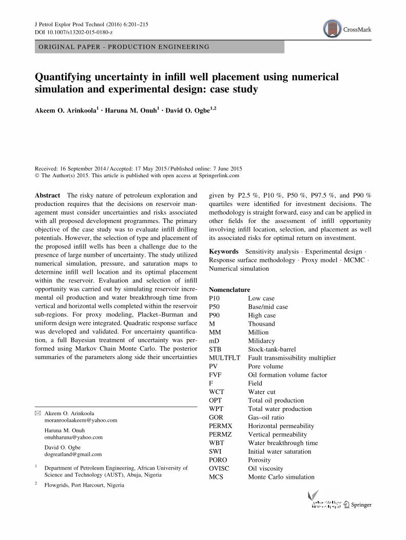
Figure 7 shows the results of the pressure, GOR, water

cut, and cumulative water matches at field level. In all

the plots, the dotted points indicate the observed data,

while the continuous line indicates the simulated values.

The pressure match is shown in black color, water cut,

and cumulative water produced in blue, while the GOR

is shown in red color. A good pressure match was

obtained an indication of adequate capturing of the

energy within the reservoir. Field-wise, the water cut

match considered satisfactory to be used for further

analysis. Figure 8 shows the distribution of the residual

oil saturation at the end of history in some layers of the

reservoir. It is obvious that beyond the life of the

existing wells, substantial residual oil saturation is left

behind. These are found between the existing wells as

well as in the intra reservoir shale breaks. Infill drilling

evaluation is a good reservoir management for this case

study.

Fig. 6 Field production

performance profiles

Fig. 5 a Reservoir energy diagram and b pressure profile with and without aquifer model

206 J Petrol Explor Prod Technol (2016) 6:201–215

123

Infill wells selection and placement

In this study, the placement of wells at different layers and

the determination of optimum horizontal length to be

perforated were done manually but guided well by layers

oil saturation map and practice within the Niger Delta. In

order to achieve a 35 % recovery factor, a number of

production schemes were considered. These include the use

of all vertical wells or all horizontal wells, or a combina-

tion of both horizontal and vertical wells. This sensitivity

study was done manually. The well placement was opti-

mized for each scheme considered by placing the wells one

at a time and running the simulation for 18 years. For the

horizontal wells, the evaluation of the vertical placement

and optimal lateral length was simulated assuming hori-

zontal length of 700 and 1000 m. The inter-well spacing

assumed was 400 m. In all the simulations, WBT and

recoverable oil are the responses.

Table 1 compares the performance of the horizontal and

vertical wells across the reservoir sub-regions as well as the

effects of the lateral length of the horizontal wells on

production and water break through time. The

recommendations to drill or not was based strictly on

number of wells, WBT, and cumulative oil recovery. The

results show that in all the recommended regions for infill

drilling horizontal wells with 1000 m lateral lengths give

higher productivity.

Drilling a horizontal well with horizontal lateral length

of 700 m in Region 1 produced additional 5 MMSTB the

same quantity obtained from 4 vertical wells in the same

region. This region can be said to be almost depleted

because the simulation result indicated no significant dif-

ference in additional reserves using 1000 and 700 m hor-

izontal well lengths. Considering additional reserves, a

horizontal well is optimum with well length of 700 m in

Regions 1 and 3. However, it was observed that all wells

(vertical and horizontal) experienced WBT 1 month after

production hence, infill drilling in Regions 1 and 3 was not

a viable option.

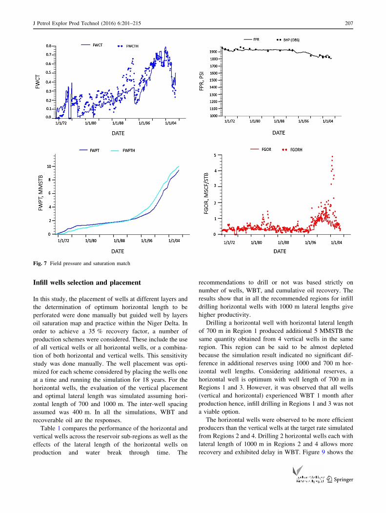
The horizontal wells were observed to be more efficient

producers than the vertical wells at the target rate simulated

from Regions 2 and 4. Drilling 2 horizontal wells each with

lateral length of 1000 m in Regions 2 and 4 allows more

recovery and exhibited delay in WBT. Figure 9 shows the

Fig. 7 Field pressure and saturation match

J Petrol Explor Prod Technol (2016) 6:201–215 207

123

incremental production and compares well performance

based on well number and type. The ‘‘8 vertical wells’’ is

the total number of vertical wells drilled and completed in

the selected two regions of the reservoir with 4 wells

drilled each to Regions 2 and 4. Likewise, total number of

four horizontal wells was drilled with two horizontal wells

drilled and completed each in the two regions.

The result of the simulation shows better performance

with four horizontal wells compared to eight vertical wells.

For optimal number of infill well required, three horizontal

wells were drilled and simulated. First, two completed in

Region 2 and one in Region 4. Then, with one horizontal well

completed in Region 2 and two horizontal wells drilled and

completed in Region 4. Region 4 was found to be more

productive than Region 2 and hence the ratio of horizontal

wells simulated in Regions 2 and 4 is 1:2. A significant dif-

ference in additional reserve was produced when compared

with the four horizontal wells. Therefore all the subsequent

analysis was done based on production results from 4 wells.

Influence of well length

The lengths of the horizontal well examined are 700, 1000,

and 1200 m for the horizontal wells. The simulation was

performed at constant flow rate of 1500 Stb/day. Figure 10

shows the sensitivity of the horizontal lateral length to

Fig. 8 Distribution of the residual oil saturation at the end of history match

Table 1 Summary of wells performance for optimum well selection and placement

Reservoir Well type No of wells Well length (m) Cum. oil (MMSTB) WBT (days) Remark

Region1 Vertical 4 NA 5 30 No infill

Horizontal 2 700 5 30

1000 5.3 30

Region2 Vertical 4 NA 5.5 549 Infill

Horizontal 2 700 5.3 1491

1000 6 1614

Region3 Vertical 4 NA 6.2 30 No Infill

Horizontal 2 700 6.2 30

1000 6.5 30

Region4 Vertical 4 NA 7 30 Infill

Horizontal 2 700 6 519

1000 7 641

NA not applicable

208 J Petrol Explor Prod Technol (2016) 6:201–215

123

incremental production. As shown in Fig. 11, there is no

significant difference in additional recovery when 1000 and

1200 m horizontal length was simulated. However, a hor-

izontal length of 1000 m shows a marked difference in

additional recovery when compare with simulated 700 m

lateral horizontal length. Based on this analysis, 2 hori-

zontal wells of 1000 m lateral length each was recom-

mended for drilling and evaluation in the Reservoir

Regions 2 and 4. The new reservoir model that included

infill wells was therefore used to quantify uncertainty

associated with the development concept.

Uncertainty quantification

The following sections described in details the workflow

the study adopted to assess uncertainty associated with

infill drilling.

Screening analysis using Placket–Burman design

(PBD)

The essence of performing this exercise was to minimize

number of simulation. All ten uncertain factors were

Fig. 11 Experimental runs

showing the degree of

uncertainty in the MM Field

(Dark line represents the base

case run)

Fig. 9 Comparison of

incremental production from

vertical and horizontal wells

Fig. 10 Sensitivity of

additional recovery to different

lateral length of the horizontal

well

J Petrol Explor Prod Technol (2016) 6:201–215 209

123

subjected to screening using PBD to select ‘‘heavy hitters’’

for response surface development. Table 2 shows all

parameters and their ranges in terms ofmultiplier on the base

case model. The multipliers were arrived at after series of

sensitivity runs to study the deflection of the response curves

from the base case position. This was achieved by either

decrease the base case value or increases it using amultiplier.

Through this process, the parameter rangeswere determined.

Using the parameters in Table 2, a PBD matrix shown in

Table 3 was constructed. The ‘‘?1’’ and ‘‘-1’’ correspond

to the absolute high and low values of the variables. The

simulation was done on the forecast reserves, and response

value was recorded for 15 and 30 years of forecast to avoid

missing out of any impactful factor. In all the runs, the

original history match is preserved.

Figure 11 shows the deviation of different runs from the

base value (thick-black color). The plot indicates the

presence of uncertainties in the production forecast. This

can seriously affects its optimal development strategies.

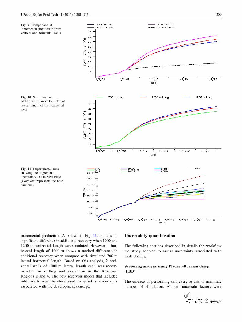
With the Analysis of variance (ANOVA), the main effects

were computed. The relative contribution of different main

factors is presented as Pareto charts in Fig. 12. There are

five ‘‘heavy-hitters’’ identified after 15 years of forecast are

OVISC, SWI, PERMX, PORO, and PERMZ. Whereas,

after 30 years of forecast, only four ‘‘heavy-hitters’’

namely: OVISC, SWI, PERMX, and PORO were identified

at 95 % analysis confidence level.

Design of experiment

Experiments are designed for different purposes. The

objectives here are to gain maximum information and for

building model that most approximated the reservoir

behavior at minimum costs. This study proposed a quad-

ratic model using the screened four (m = 4) variables

which will require at least a total of 15 experiments

[P = (m ? 1)(m ? 2)/2]. The goal here is to select best

design without compromising the efficiency. Consider that

it is desired to utilize the 4 identified decision variables

with each factor has 16 levels (discretized possible values

Table 2 Experimental range in terms of multipliers on the base case uncertain parameters

S. no. Parameters Keywords Minimum value Base case Maximum value

1 Oil viscosity OVISC 0.90 1 1.10

2 Horizontal permeability PERMX 0.57 1 1.29

3 Vertical permeability PERMZ 0.50 1 6.00

4 Porosity PORO 0.90 1 1.10

5 Critical gas saturation SGCR 0.50 1 1.50

6 Critical water saturation SWCR 0.53 1 1.07

7 Fault transmissibility multiplier MULTFLT 0.50 1 2.00

8 Water relative permeability KRW (SORW) 0.36 1 1.25

9 Initial water saturation SWI 0.65 1 0.90

10 Aquifer pore volume AQUIPV 0.85 1 1.35

Table 3 PB design table for 10 parameters

Run A:OVISC B:PERMX C:PERMZ D:PORO E:SGCR F:SWCR G:MULTFL H:KRW J:ISW K:AQUPV FOPT

(15 years)

FOPT

(30 years)

1 -1 -1 -1 1 1 1 -1 1 1 -1 30,848,400 33,479,500

2 1 -1 1 1 -1 1 -1 -1 -1 1 27,154,800 29,412,400

3 1 1 1 -1 1 1 -1 1 -1 -1 28,005,900 29,769,600

4 1 1 -1 1 1 -1 1 -1 -1 -1 27,889,000 30,076,700

5 -1 -1 1 1 1 -1 1 1 -1 1 30,629,500 33,815,700

6 -1 -1 -1 -1 -1 -1 -1 -1 -1 -1 26,898,400 28,727,400

7 1 -1 1 -1 -1 -1 1 1 1 -1 28,034,500 29,923,100

8 1 -1 -1 -1 1 1 1 -1 1 1 27,275,300 29,486,200

9 -1 1 1 -1 1 -1 -1 -1 1 1 32,087,300 35,060,000

10 -1 1 -1 -1 -1 1 1 1 -1 1 30,096,500 32,551,700

11 -1 1 1 1 -1 1 1 -1 1 -1 33,201,400 36,053,900

12 1 1 -1 1 -1 -1 -1 1 1 1 30,582,600 33,411,100

210 J Petrol Explor Prod Technol (2016) 6:201–215

123

of parameters). The total of all possible combinations is

164 = 65,536. Orthogonal test designs can reduce test

number to 162 = 256; uniform design (UD), however, can

reduce it to only 16 tests. This is an advantage of modern

experimental design over the conventional designs like

central composite, Box–Behnken, and full factorial designs.

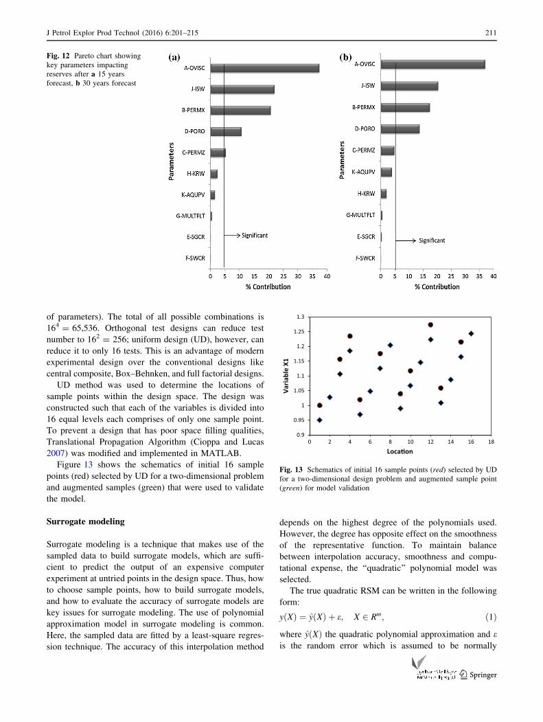
UD method was used to determine the locations of

sample points within the design space. The design was

constructed such that each of the variables is divided into

16 equal levels each comprises of only one sample point.

To prevent a design that has poor space filling qualities,

Translational Propagation Algorithm (Cioppa and Lucas

2007) was modified and implemented in MATLAB.

Figure 13 shows the schematics of initial 16 sample

points (red) selected by UD for a two-dimensional problem

and augmented samples (green) that were used to validate

the model.

Surrogate modeling

Surrogate modeling is a technique that makes use of the

sampled data to build surrogate models, which are suffi-

cient to predict the output of an expensive computer

experiment at untried points in the design space. Thus, how

to choose sample points, how to build surrogate models,

and how to evaluate the accuracy of surrogate models are

key issues for surrogate modeling. The use of polynomial

approximation model in surrogate modeling is common.

Here, the sampled data are fitted by a least-square regres-

sion technique. The accuracy of this interpolation method

depends on the highest degree of the polynomials used.

However, the degree has opposite effect on the smoothness

of the representative function. To maintain balance

between interpolation accuracy, smoothness and compu-

tational expense, the ‘‘quadratic’’ polynomial model was

selected.

The true quadratic RSM can be written in the following

form:

y Xð Þ ¼ y Xð Þ þ e; X 2 Rm; ð1Þ

where y Xð Þ the quadratic polynomial approximation and eis the random error which is assumed to be normally

Fig. 12 Pareto chart showing

key parameters impacting

reserves after a 15 years

forecast, b 30 years forecast

0.9

0.95

1

1.05

1.1

1.15

1.2

1.25

1.3

0 2 4 6 8 10 12 14 16 18

Varia

ble

X1

Loca�on

Fig. 13 Schematics of initial 16 sample points (red) selected by UD

for a two-dimensional design problem and augmented sample point

(green) for model validation

J Petrol Explor Prod Technol (2016) 6:201–215 211

123

distributed with mean zero and variance of r2. The error eiat each observation is supposed to be independent and

identically distributed (iid).

The modeled quadratic RSM predictor y Xð Þ is defined as:

y Xð Þ ¼ b0 þXm

i¼1

bixi þXm

i¼1

biix2i þ

Xm

i¼1

Xm

j� i

bijxixj; ð2Þ

where b0; bi; bii and bij are the unknown coefficients.

Let beRm be the column vector contains these P

unknown coefficients. The least square estimator of b is

b ¼ ðUTUÞ�1UTys; ð3Þ

where

U ¼1

..

.

1

xð1Þ1 � � � x

ð1Þm

..

. . .. ..

.

xðnÞ1 � � � x

ðnÞm

xð1Þ1 x

ð1Þ2

..

.

xðnÞ1 x

ðnÞ2

. . .

. ..

. . .

xð1Þm�1x

ð1Þm

..

.

xðnÞm�1x

ðnÞm

ðxð1Þ1 Þ2

..

.

ðxðnÞ1 Þ2

. . .

. ..

. . .

ðxð1Þm Þ2

..

.

ðxðnÞm Þ2

2

664

3

775

2 RnXp

ð4Þ

and ys are observations; b0 ¼ 2:488; b1 ¼ 53:0332 and

b2 ¼ �17:2437: The approximated response yðXÞ at any

untried x can be efficiently predicted by Eq. (5).

y Xð Þ MMstb½ � ¼ b0 þ b1SWIþ b2PERMX2: ð5Þ

The cross plot of the model prediction against the actual

experimental value is shown in Fig. 14. On this plot, the

vast majority of the points is along the x = y line. This

shows that the predictions were a perfect fit of the

experimental data.

Evaluation of approximation models

Relative error (RE) and root mean squared error (RMSE)

were used to evaluate the error of the approximation

models at test points other than those used in building the

model. The test points comprises of ten new sample points

within the sample space. These points are shown as green

doted points augmented in the original design in Fig. 13.

The relative error is

�e ¼ 1

nt

Xnt

i¼1

eðiÞ; where; eðiÞ ¼ yðiÞt � y

ðiÞt

yðiÞt

ð6Þ

nt is number of the test points; yt(i) and �y

ðiÞt are the true value

and predicted value corresponding to the ith test point,

respectively.

The RMSE is defined by

re ¼

ffiffiffiffiffiffiffiffiffiffiffiffiffiffiffiffiffiffiffiffiffiffiffiPnti¼1ðeðiÞÞ

2

nt

s

: ð7Þ

Table 4 shows the result obtained from statistical error

analysis. The low (RMSE = 1.05) value indicates a good

model. Approximately zero value of average absolute

percentage relative error (AAPRE = 0.76 %) recorded

indicates relative low absolute deviation in percent from

the experimental values. Hence, implies a better

correlation.

Markov Chain Monte Carlo (MCMC) simulation

In order to quantify the uncertainty on production forecast

the Bayesian parameter estimation conditioned on histori-

cal information was done using the software Winbugs

(Spiegelhalter et al. 2000). This requires a prior distribution

for the parameters and the likelihood function. Winbugs

has a built-in likelihood function for uncensored and cen-

sored normal data that were used in these simulations.

Parameter estimation is made from updating with the

prior distribution to compute the posterior distribution

using Bayes’ Theorem.

p h=D

� �¼

f D=h� �

eðhÞr f D=h

� �e hð Þdh

; ð8Þ

R² = 0.9879

26

27

28

29

30

31

32

26 27 28 29 30 31 32

Pred

ic�o

n (M

Mst

b)

Experimental (MMstb)

Fig. 14 Comparison of the actual experimental value and model

predicted values

Table 4 Statistical error analysis

Experimental Prediction Residual AD % Error MSE

27.70 27.67 0.03 0.03 0.12 0.01

30.55 30.15 0.40 0.40 1.32 1.75

31.43 31.07 0.36 0.36 1.13 1.28

28.15 28.03 0.13 0.13 0.45 0.20

30.46 30.40 0.07 0.07 0.21 0.05

28.41 28.37 0.04 0.04 0.15 0.02

29.50 29.61 -0.10 0.10 -0.35 0.12

31.12 31.45 -0.33 0.33 -1.07 1.14

29.44 28.70 0.74 0.74 2.53 6.39

30.94 30.86 0.08 0.08 0.25 0.06

212 J Petrol Explor Prod Technol (2016) 6:201–215

123

where p h=D

� �the posterior distribution of the parameters h

is, f D=h

� �is the likelihood function, and e(h) is the prior

distribution of h. The denominator is a normalizing con-

stant that scales the posterior so that the area under the

posterior pdf equals one.

The stochastic parameters b0; b1; b2 and s are given

proper prior distributions, while the logical expression for

r allows the standard deviation to be estimated. To check

the convergence of MCMC simulations, multiple chains

with divergent starting points were run using derivative-

free adaptive rejection sampling algorithm.

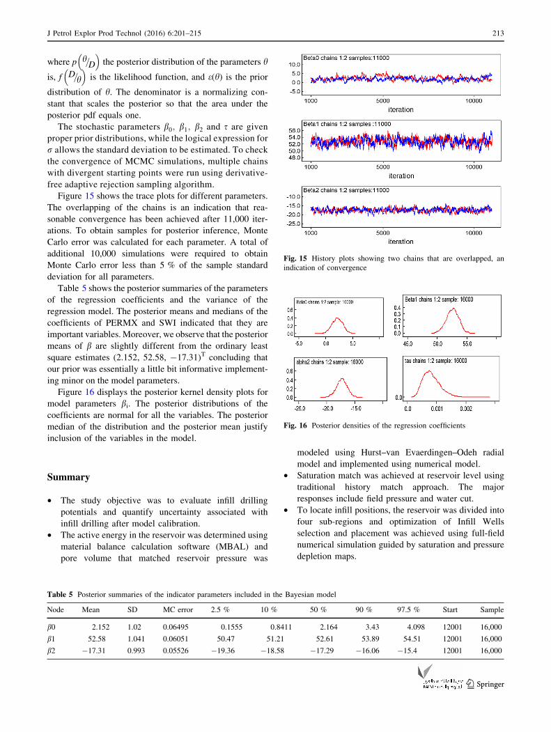
Figure 15 shows the trace plots for different parameters.

The overlapping of the chains is an indication that rea-

sonable convergence has been achieved after 11,000 iter-

ations. To obtain samples for posterior inference, Monte

Carlo error was calculated for each parameter. A total of

additional 10,000 simulations were required to obtain

Monte Carlo error less than 5 % of the sample standard

deviation for all parameters.

Table 5 shows the posterior summaries of the parameters

of the regression coefficients and the variance of the

regression model. The posterior means and medians of the

coefficients of PERMX and SWI indicated that they are

important variables. Moreover, we observe that the posterior

means of b are slightly different from the ordinary least

square estimates (2.152, 52.58, -17.31)T concluding that

our prior was essentially a little bit informative implement-

ing minor on the model parameters.

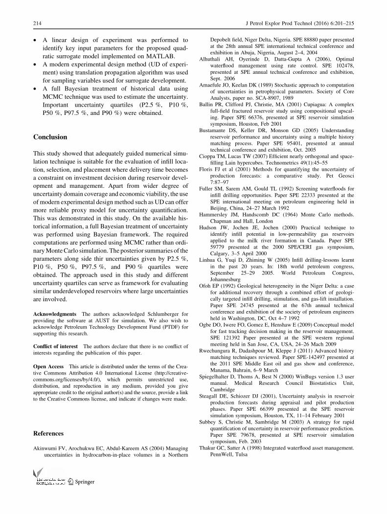
Figure 16 displays the posterior kernel density plots for

model parameters bi. The posterior distributions of the

coefficients are normal for all the variables. The posterior

median of the distribution and the posterior mean justify

inclusion of the variables in the model.

Summary

• The study objective was to evaluate infill drilling

potentials and quantify uncertainty associated with

infill drilling after model calibration.

• The active energy in the reservoir was determined using

material balance calculation software (MBAL) and

pore volume that matched reservoir pressure was

modeled using Hurst–van Evaerdingen–Odeh radial

model and implemented using numerical model.

• Saturation match was achieved at reservoir level using

traditional history match approach. The major

responses include field pressure and water cut.

• To locate infill positions, the reservoir was divided into

four sub-regions and optimization of Infill Wells

selection and placement was achieved using full-field

numerical simulation guided by saturation and pressure

depletion maps.

Fig. 15 History plots showing two chains that are overlapped, an

indication of convergence

Table 5 Posterior summaries of the indicator parameters included in the Bayesian model

Node Mean SD MC error 2.5 % 10 % 50 % 90 % 97.5 % Start Sample

b0 2.152 1.02 0.06495 0.1555 0.8411 2.164 3.43 4.098 12001 16,000

b1 52.58 1.041 0.06051 50.47 51.21 52.61 53.89 54.51 12001 16,000

b2 -17.31 0.993 0.05526 -19.36 -18.58 -17.29 -16.06 -15.4 12001 16,000

Fig. 16 Posterior densities of the regression coefficients

J Petrol Explor Prod Technol (2016) 6:201–215 213

123

• A linear design of experiment was performed to

identify key input parameters for the proposed quad-

ratic surrogate model implemented on MATLAB.

• A modern experimental design method (UD of experi-

ment) using translation propagation algorithm was used

for sampling variables used for surrogate development.

• A full Bayesian treatment of historical data using

MCMC technique was used to estimate the uncertainty.

Important uncertainty quartiles (P2.5 %, P10 %,

P50 %, P97.5 %, and P90 %) were obtained.

Conclusion

This study showed that adequately guided numerical simu-

lation technique is suitable for the evaluation of infill loca-

tion, selection, and placement where delivery time becomes

a constraint on investment decision during reservoir devel-

opment and management. Apart from wider degree of

uncertainty domain coverage and economic viability, the use

of modern experimental designmethod such as UD can offer

more reliable proxy model for uncertainty quantification.

This was demonstrated in this study. On the available his-

torical information, a full Bayesian treatment of uncertainty

was performed using Bayesian framework. The required

computations are performed using MCMC rather than ordi-

naryMonteCarlo simulation. The posterior summaries of the

parameters along side thir uncertainties given by P2.5 %,

P10 %, P50 %, P97.5 %, and P90 % quartiles were

obtained. The approach used in this study and different

uncertainty quartiles can serve as framework for evaluating

similar underdeveloped reservoirs where large uncertainties

are involved.

Acknowledgments The authors acknowledged Schlumberger for

providing the software at AUST for simulation. We also wish to

acknowledge Petroleum Technology Development Fund (PTDF) for

supporting this research.

Conflict of interest The authors declare that there is no conflict of

interests regarding the publication of this paper.

Open Access This article is distributed under the terms of the Crea-

tive Commons Attribution 4.0 International License (http://creative-

commons.org/licenses/by/4.0/), which permits unrestricted use,

distribution, and reproduction in any medium, provided you give

appropriate credit to the original author(s) and the source, provide a link

to the Creative Commons license, and indicate if changes were made.

References

Akinwumi FV, Arochukwu EC, Abdul-Kareem AS (2004) Managing

uncertainties in hydrocarbon-in-place volumes in a Northern

Depobelt field, Niger Delta, Nigeria. SPE 88880 paper presented

at the 28th annual SPE international technical conference and

exhibition in Abuja, Nigeria, August 2–4, 2004

Alhuthali AH, Oyerinde D, Datta-Gupta A (2006), Optimal

waterflood management using rate control. SPE 102478,

presented at SPE annual technical conference and exhibition,

Sept. 2006

Amaefule JO, Keelan DK (1989) Stochastic approach to computation

of uncertainties in petrophysical parameters. Society of Core

Analysts, paper no. SCA-8907, 1989

Ballin PR, Clifford PJ, Christie, MA (2001) Cupiagua: A complex

full-field fractured reservoir study using compositional upscal-

ing. Paper SPE 66376, presented at SPE reservoir simulation

symposium, Houston, Feb 2001

Bustamante DS, Keller DR, Monson GD (2005) Understanding

reservoir performance and uncertainty using a multiple history

matching process. Paper SPE 95401, presented at annual

technical conference and exhibition, Oct. 2005

Cioppa TM, Lucas TW (2007) Efficient nearly orthogonal and space-

filling Lain hypercubes. Technometrics 49(1):45–55

Floris FJ et al (2001) Methods for quantifying the uncertainty of

production forecasts: a comparative study. Pet Geosci

7:87–97

Fuller SM, Sarem AM, Gould TL (1992) Screening waterfloods for

infill drilling opportunities. Paper SPE 22333 presented at the

SPE international meeting on petroleum engineering held in

Beijing, China, 24–27 March 1992

Hammersley JM, Handscomb DC (1964) Monte Carlo methods.

Chapman and Hall, London

Hudson JW, Jochen JE, Jochen (2000) Practical technique to

identify infill potential in low-permeability gas reservoirs

applied to the milk river formation in Canada. Paper SPE

59779 presented at the 2000 SPE/CERI gas symposium,

Calgary, 3–5 April 2000

Linhua G, Yuqi D, Zhiming W (2005) Infill drilling-lessons learnt

in the past 20 years. In: 18th world petroleum congress,

September 25–29 2005. World Petroleum Congress,

Johannesburg

Ofoh EP (1992) Geological heterogeneity in the Niger Delta: a case

for additional recovery through a combined effort of geologi-

cally targeted infill drilling, stimulation, and gas-lift installation.

Paper SPE 24745 presented at the 67th annual technical

conference and exhibition of the society of petroleum engineers

held in Washington, DC, Oct 4–7 1992

Ogbe DO, Iwere FO, Gomez E, Henshaw E (2009) Conceptual model

for fast tracking decision making in the reservoir management.

SPE 121392 Paper presented at the SPE western regional

meeting held in San Jose, CA, USA, 24–26 Mach 2009

Rwechungura R, Dadashpour M, Kleppe J (2011) Advanced history

matching techniques reviewed. Paper SPE-142497 presented at

the 2011 SPE Middle East oil and gas show and conference,

Manama, Bahrain, 6–9 March

Spiegelhalter D, Thoms A, Best N (2000) WinBugs version 1.3 user

manual. Medical Research Council Biostatistics Unit,

Cambridge

Steagall DE, Schiozer DJ (2001), Uncertainty analysis in reservoir

production forecasts during appraisal and pilot production

phases. Paper SPE 66399 presented at the SPE reservoir

simulation symposium, Houston, TX, 11–14 February 2001

Subbey S, Christie M, Sambridge M (2003) A strategy for rapid

quantification of uncertainty in reservoir performance prediction.

Paper SPE 79678, presented at SPE reservoir simulation

symposium, Feb. 2003

Thakur GC, Satter A (1998) Integrated waterflood asset management.

PennWell, Tulsa

214 J Petrol Explor Prod Technol (2016) 6:201–215

123

Venkataraman R (2000) Application of the method of experimental

design to quantify uncertainty in production profiles. Paper SPE

59422 presented at the SPE Asia Pacific conference on

integrated modelling for asset management, Yokohama, Japan,

25–26 April 2000

Voneiff GW, Cipolla C (1996) A new approach to large-scale infill

evaluations applied to the Ozona (Canyon) gas field. Paper SPE

35203 presented at the 1996 SPE Permian oil and gas recovery

conference, Midland, 7–29 March 1996

J Petrol Explor Prod Technol (2016) 6:201–215 215

123