Quantifying Uncertainty in Real Time Performance Measurement for Highway Winter Maintenance Operations – Phase 2

Final ReportOctober 2014

Sponsored byIowa Department of TransportationFederal Highway Administration(InTrans Project 13-388)

About the Institute for Transportation

The mission of the Institute for Transportation (InTrans) at Iowa State University is to develop and implement innovative methods, materials, and technologies for improving transportation efficiency, safety, reliability, and sustainability while improving the learning environment of students, faculty, and staff in transportation-related fields.

Disclaimer Notice

The contents of this report reflect the views of the authors, who are responsible for the facts and the accuracy of the information presented herein. The opinions, findings and conclusions expressed in this publication are those of the authors and not necessarily those of the sponsors.

The sponsors assume no liability for the contents or use of the information contained in this document. This report does not constitute a standard, specification, or regulation.

The sponsors do not endorse products or manufacturers. Trademarks or manufacturers’ names appear in this report only because they are considered essential to the objective of the document.

Non-Discrimination Statement

Iowa State University does not discriminate on the basis of race, color, age, religion, national origin, pregnancy, sexual orientation, gender identity, genetic information, sex, marital status, disability, or status as a U.S. veteran. Inquiries regarding non-discrimination policies may be directed to Office of Equal Opportunity, Title IX/ADA Coordinator and Affirmative Action Officer, 3350 Beardshear Hall, Ames, Iowa 50011, 515-294-7612, eooffice@iastate.edu.

Iowa Department of Transportation Statements

Federal and state laws prohibit employment and/or public accommodation discrimination on the basis of age, color, creed, disability, gender identity, national origin, pregnancy, race, religion, sex, sexual orientation or veteran’s status. If you believe you have been discriminated against, please contact the Iowa Civil Rights Commission at 800-457-4416 or the Iowa Department of Transportation affirmative action officer. If you need accommodations because of a disability to access the Iowa Department of Transportation’s services, contact the agency’s affirmative action officer at 800-262-0003.

The preparation of this report was financed in part through funds provided by the Iowa Department of Transportation through its “Second Revised Agreement for the Management of Research Conducted by Iowa State University for the Iowa Department of Transportation” and its amendments.

The opinions, findings, and conclusions expressed in this publication are those of the authors and not necessarily those of the Iowa Department of Transportation or the U.S. Department of Transportation.

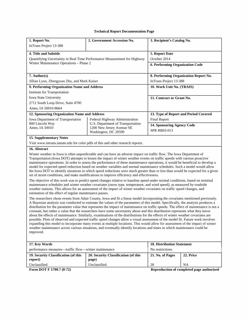
Technical Report Documentation Page

1. Report No. 2. Government Accession No. 3. Recipient’s Catalog No. InTrans Project 13-388

4. Title and Subtitle 5. Report Date Quantifying Uncertainty in Real Time Performance Measurement for Highway Winter Maintenance Operations – Phase 2

October 2014 6. Performing Organization Code

7. Author(s) 8. Performing Organization Report No. Jillian Lyon, Zhengyuan Zhu, and Mark Kaiser InTrans Project 13-388 9. Performing Organization Name and Address 10. Work Unit No. (TRAIS) Institute for Transportation Iowa State University 2711 South Loop Drive, Suite 4700 Ames, IA 50010-8664

11. Contract or Grant No.

12. Sponsoring Organization Name and Address 13. Type of Report and Period Covered Iowa Department of Transportation 800 Lincoln Way Ames, IA 50010

Federal Highway Administration U.S. Department of Transportation 1200 New Jersey Avenue SE Washington, DC 20590

Final Report 14. Sponsoring Agency Code SPR RB03-013

15. Supplementary Notes Visit www.intrans.iastate.edu for color pdfs of this and other research reports. 16. Abstract Winter weather in Iowa is often unpredictable and can have an adverse impact on traffic flow. The Iowa Department of Transportation (Iowa DOT) attempts to lessen the impact of winter weather events on traffic speeds with various proactive maintenance operations. In order to assess the performance of these maintenance operations, it would be beneficial to develop a model for expected speed reduction based on weather variables and normal maintenance schedules. Such a model would allow the Iowa DOT to identify situations in which speed reductions were much greater than or less than would be expected for a given set of storm conditions, and make modifications to improve efficiency and effectiveness. The objective of this work was to predict speed changes relative to baseline speed under normal conditions, based on nominal maintenance schedules and winter weather covariates (snow type, temperature, and wind speed), as measured by roadside weather stations. This allows for an assessment of the impact of winter weather covariates on traffic speed changes, and estimation of the effect of regular maintenance passes. The researchers chose events from Adair County, Iowa and fit a linear model incorporating the covariates mentioned previously. A Bayesian analysis was conducted to estimate the values of the parameters of this model. Specifically, the analysis produces a distribution for the parameter value that represents the impact of maintenance on traffic speeds. The effect of maintenance is not a constant, but rather a value that the researchers have some uncertainty about and this distribution represents what they know about the effects of maintenance. Similarly, examinations of the distributions for the effects of winter weather covariates are possible. Plots of observed and expected traffic speed changes allow a visual assessment of the model fit. Future work involves expanding this model to incorporate many events at multiple locations. This would allow for assessment of the impact of winter weather maintenance across various situations, and eventually identify locations and times in which maintenance could be improved.

17. Key Words 18. Distribution Statement performance measures—traffic flow—winter maintenance No restrictions. 19. Security Classification (of this report)

20. Security Classification (of this page)

21. No. of Pages 22. Price

Unclassified. Unclassified. 28 NA Form DOT F 1700.7 (8-72) Reproduction of completed page authorized

QUANTIFYING UNCERTAINTY IN REAL TIME PERFORMANCE MEASUREMENT FOR HIGHWAY WINTER MAINTENANCE OPERATIONS – PHASE 2

Final Report October 2014

Principal Investigator

Zhengyuan Zhu Associate Professor, Department of Statistics, Iowa State University

Co-Principal Investigator

Mark Kaiser Professor and Director of Graduate Education, Department of Statistics, Iowa State University

Research Assistant

Jillian Lyon

Authors Jillian Lyon, Zhengyuan Zhu, and Mark Kaiser

Sponsored by the Iowa Department of Transportation

and the Federal Highway Administration (SPR RB03-013)

Preparation of this report was financed in part

through funds provided by the Iowa Department of Transportation through its Research Management Agreement with the

Institute for Transportation (InTrans Project 13-388)

A report from Institute for Transportation

Iowa State University 2711 South Loop Drive, Suite 4700

Ames, IA 50010-8664 Phone: 515-294-8103 Fax: 515-294-0467

www.intrans.iastate.edu

TABLE OF CONTENTS

ACKNOWLEDGMENTS ............................................................................................................. ix

EXECUTIVE SUMMARY ........................................................................................................... xi

INTRODUCTION AND OVERVIEW ...........................................................................................1

PREVIOUS MODEL FOR SPEED REDUCTION .........................................................................2

Review of Sequential Bayesian Model ................................................................................2 Modifications to Sequential Bayesian Model ......................................................................2 Effect of Modifications ........................................................................................................3

EXPERT SURVEY .........................................................................................................................5

Survey Background ..............................................................................................................5 Survey Results .....................................................................................................................6

EXPLORATORY ANALYSIS OF SENSOR DATA .....................................................................8

Baseline Traffic Trends........................................................................................................8 Variable Exploration and Basic Linear Model ....................................................................9

HIERARCHICAL MODEL FOR ADAIR EVENTS ....................................................................11

Format of Data ...................................................................................................................11 Nominal Plot Times ...........................................................................................................11 Model Formulation ............................................................................................................11 Implementation of the Model.............................................................................................12

POTENTIAL DIRECTIONS AND FUTURE WORK .................................................................15

REFERENCES ..............................................................................................................................17

v

LIST OF FIGURES

Figure 1. Continuous approximations to the temperature effect using a logistic curve (left) and the new approach with more variability (right) ...................................................................3

Figure 2. Predicted traffic speed using the old dynamic Bayesian model (left) and using the new model (right) with the x-axis representing two minute intervals starting at 8:00 a.m. ........4

Figure 3. Speed reduction ranges for 11 experts for interstate roads during peak traffic times when there is moderate snow fall and the temperature is between 15 and 28 degrees Fahrenheit: two panels have rain prior (bottom) while two do not (top) and two panels (left) have wind speed greater than 15 mph while two panels (right) have wind speeds less than 15 mph...................................................................................................................7

Figure 4. Observed traffic speeds for March 14, 2011 through March 20, 2011 at three locations: Davenport (top left), Hanlontown (top right), and Newton (bottom) ..................................8

Figure 5. Absolute deviation from freezing against speed reduction for three interstate locations during snow events ..............................................................................................................9

Figure 6. Observed speed reduction from baseline (black line), predicted speed reduction from baseline using linear model (blue line), and predicted speed reduction from baseline using Qiu and Nixon’s model (red line) for three winter weather events in Adair County, Iowa10

Figure 7. Model fitted to snow event in Adair County where x-axis represents 10 minute intervals starting at 10:31 a.m. on January 9, 2011 and ending at 11:49 p.m. on January 10, 2011 and blue dotted lines are 90 percent error bounds ..............................................13

Figure 8. Expected value of speed reduction from model fitted to snow event in Adair County where the horizontal axis represents 10 minute intervals starting at 10:31 a.m. on January 9, 2011 and ending at 11:49 p.m. on January 10, 2011 and blue dotted lines are 90 percent error bounds ..........................................................................................................14

LIST OF TABLES

Table 1. Number of garages receiving surveys and number of surveys returned ............................5 Table 2. Parameter estimates based on the model fit to a snow event starting at 10:31 a.m. on

January 9, 2011 and ending on January 10, 2011 in Adair County ...................................14

vii

ACKNOWLEDGMENTS

The authors would like to thank the Iowa Department of Transportation for sponsoring this research and the Federal Highway Administration for state planning and research (SPR) funds used for this project. The authors would also like to thank everyone who assisted on this project, and especially Tina Greenfield.

ix

EXECUTIVE SUMMARY

Winter weather in Iowa is often unpredictable and can have an adverse impact on traffic flow. The Iowa Department of Transportation (Iowa DOT) attempts to lessen the impact of winter weather events on traffic speeds with various proactive maintenance operations. In order to assess the performance of these maintenance operations, it would be beneficial to develop a model for expected speed reduction based on weather variables and normal maintenance schedules. Such a model would allow the Iowa DOT to identify situations in which speed reductions were much greater than or less than would be expected for a given set of storm conditions, and make modifications to improve efficiency and effectiveness. The objective of this work was to predict speed changes relative to baseline speed under normal conditions, based on nominal maintenance schedules and winter weather covariates (snow type, temperature, and wind speed), as measured by roadside weather stations. This allows for an assessment of the impact of winter weather covariates on traffic speed changes, and estimation of the effect of regular maintenance passes. The researchers chose events from Adair County, Iowa and fit a linear model incorporating the covariates mentioned previously. A Bayesian analysis was conducted to estimate the values of the parameters of this model. Specifically, the analysis produces a distribution for the parameter value that represents the impact of maintenance on traffic speeds. The effect of maintenance is not a constant, but rather a value that the researchers have some uncertainty about and this distribution represents what they know about the effects of maintenance. Similarly, examinations of the distributions for the effects of winter weather covariates are possible. Plots of observed and expected traffic speed changes allow a visual assessment of the model fit. Future work involves expanding this model to incorporate many events at multiple locations. This would allow for assessment of the impact of winter weather maintenance across various situations, and eventually identify locations and times in which maintenance could be improved.

xi

INTRODUCTION AND OVERVIEW

Winter weather in Iowa is often unpredictable and can have a large impact on traffic flow. The Iowa Department of Transportation (DOT) attempts to lessen the impact of winter weather events on traffic speeds with various maintenance operations. In order to assess the performance of these maintenance operations, it is necessary to come up with a model for expected speed reduction based on different winter weather variables and normal maintenance schedules. Such a model would allow the Iowa DOT to identify situations where speed reductions were much greater than they should have been for a given set of storm conditions.

In 2009, Qiu and Nixon developed a model to predict speed reduction. This model was then modified in 2011 by Greenfield et al. The researchers reviewed these previously developed models as well as discussed further modifications to introduce more variability into the model inputs. Although these modifications were an improvement, they still needed to account for variability in the model structure itself.

To get an idea about the impact of individual weather covariates on speed reduction, an expert survey was developed with the goal of using the survey results to incorporate variability into the structure of the previous model. However, problems in the survey such as low response rate, contradictory responses, and wide ranges of responses led the researchers to conclude that a more data-driven approach is necessary. An exploratory analysis of the sensor data was used to help formulate a hierarchical model for storm events at individual locations. The developed dynamic linear regression model takes into account winter weather variables as well as plow operation schedules, which makes it different from the previous models. Also, the researchers used deviation from “normal” traffic speeds as their response instead of deviation from the posted speed limit. Using temperature in the model as measured by the absolute deviation from freezing as opposed to using the raw temperature value shows how this new model does a good job predicting the expected value of speed reduction and capturing the inherent variability of the data. Finally, they discuss the future work to be done and how the research model can be expanded to multiple locations.

1

PREVIOUS MODEL FOR SPEED REDUCTION

Review of Sequential Bayesian Model

In 2009, Qiu and Nixon developed a model for speed reduction at time (𝑡𝑡). This model uses storm precipitation, surface temperature, wind speed, and whether or not the storm started as rain to predict the speed reduction from the posted speed limit at a given location. In this model, the values of the covariates were completely determined by the conditions at time (𝑡𝑡) and did not take into account previous storm conditions.

In 2011, Greenfield et al. changed the original model to take into account the dynamic nature of the sensor data. A distributional form was placed on each of the covariates, including storm type, surface temperature, and wind speed. Specifically, a multinomial distribution was used to model storm type. A Dirichlet prior distribution was put on the parameter vector of the multinomial distribution and a modified sequential Bayesian approach was used to estimate the probability of each storm type at time (𝑡𝑡). In this modified sequential Bayesian approach, the previous values of storm type were used, with more weight being given to more recent observations. Once an estimate of the probabilities of each storm type at time (𝑡𝑡) was obtained, it was used to simulate a storm type at time (𝑡𝑡), which was in turn used to simulate a rate of snowfall. Snowfall rates were combined to get an estimate of the accumulated snow over the past hour. This accumulation estimate was used as an input into a function that estimated the effect of storm type on traffic speed reduction.

A normal model was used for both wind speed and temperature. For these variables, it was assumed that the normal model had a constant variance and the prior distribution placed on the mean was normal. Thus, the posterior distribution for the mean of the normal model was also normal. An observation was simulated from a normal distribution with a mean equal to the posterior mean and the variance equal to the constant variance that was assumed to be known. This simulated value was then inputted into the appropriate function to produce an estimate of the effect of surface temperature or wind speed on traffic speed reduction.

Greenfield et al. showed that their dynamic Bayesian approach to modeling storm type, surface temperature, and wind speed provided better estimates of speed reduction at time (𝑡𝑡) than the deterministic functions used by Qiu and Nixon. However, the biggest drawback of the dynamic Bayesian approach is that it does not take into account variability in the structure model, which leads to confidence bands that are too narrow.

Modifications to Sequential Bayesian Model

In an attempt to introduce more variability into the dynamic Bayesian model, several changes were made to the functions that determined the effect of storm type, surface temperature, and wind speed on traffic speed reduction. First, the input for the function that estimates the effect of surface temperature was only allowed to take on values between -10 degrees Fahrenheit and 40 degrees Fahrenheit. Similarly, the input for the function that estimates the effect of wind speed

2

was allowed to vary between 0 mph and 40 mph. The changes made to the bounds on these functions were to ensure that the values of temperature and wind speed used were consistent with observable data values.

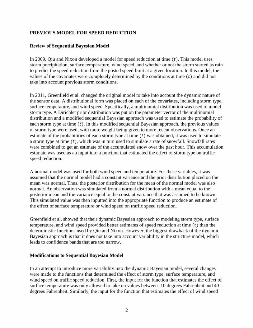
The functional form for the effect of surface temperature was also changed. Before, given a value of surface temperature, the effect was uniquely determined. To introduce more variability and still stay true to the original step function presented by Qiu and Nixon, the endpoints of the step function were connected to create an upper and lower bound for the value of the temperature effect. Thus, once a temperature value was obtained using the dynamic Bayesian approach, the temperature effect was generated from a uniform distribution with upper and lower bounds determined by the temperature value being used. As an example, suppose a temperature value of 20 degrees Fahrenheit was simulated. Using the logistic curve approximation developed by Greenfield et al., the value of the temperature effect would be 0.9186. Using this new method, the value of the temperature effect would be simulated from a uniform distribution with a lower bound of 0.7 and upper bound of 1.25. An example of this can be seen in Figure 1.

Figure 1. Continuous approximations to the temperature effect using a logistic curve (left)

and the new approach with more variability (right)

A similar procedure was used for the effect of wind speed and the effect of storm type.

Effect of Modifications

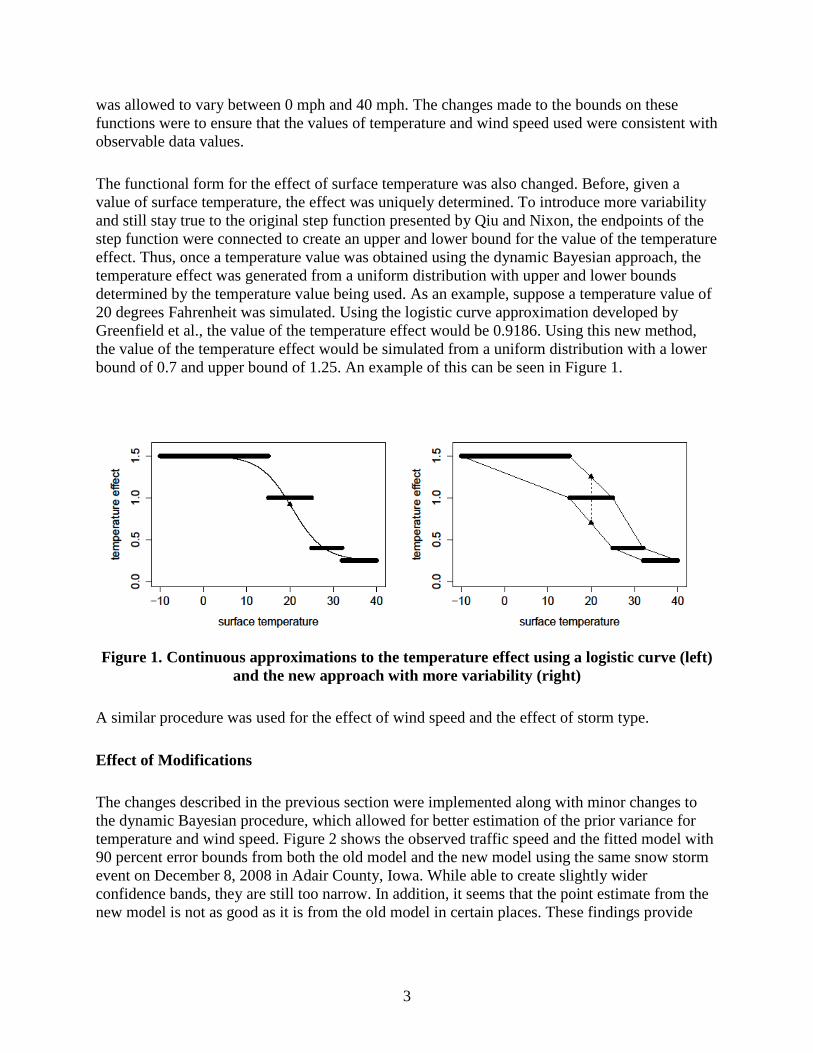
The changes described in the previous section were implemented along with minor changes to the dynamic Bayesian procedure, which allowed for better estimation of the prior variance for temperature and wind speed. Figure 2 shows the observed traffic speed and the fitted model with 90 percent error bounds from both the old model and the new model using the same snow storm event on December 8, 2008 in Adair County, Iowa. While able to create slightly wider confidence bands, they are still too narrow. In addition, it seems that the point estimate from the new model is not as good as it is from the old model in certain places. These findings provide

3

evidence that uncertainty needs to be built into the form of the original model developed by Qiu and Nixon rather than only accounting for variability in the model inputs.

Figure 2. Predicted traffic speed using the old dynamic Bayesian model (left) and using the

new model (right) with the x-axis representing two minute intervals starting at 8:00 a.m.

4

EXPERT SURVEY

Survey Background

The model for speed reduction has the effects of storm type, surface temperature, and wind speed entering only through a three-way interaction of these explanatory variables (Qiu and Nixon 2009). While wanting to investigate if the two-way interactions or the individual covariates themselves had an impact on speed reduction, the researchers were also interested in the distributional form of the speed reduction at given levels of the explanatory variables. Being able to identify the distributional form of the speed reduction would allow uncertainty to be built into the model as a whole. The original model from Qiu and Nixon was developed using surveys taken from crews following the end of a storm event. While unable to obtain the original surveys, the researchers decided to create their own survey in an attempt to elicit information from experts on winter weather road maintenance.

With the help of Tina Greenfield as well as some garage supervisors, they were able to develop a survey that contained questions regarding speed reduction in various winter weather situations. Each situation varied by type of road (interstate, class B4, class B2, or class C), time of day (peak or not), wind speed (<15 mph or >15 mph), rain prior to snow (yes or no), rate of snow fall (light, moderate, heavy), and surface temperature (<15 degrees Fahrenheit, 15-28 degrees Fahrenheit, 28-32 degrees Fahrenheit, ≥32 degrees Fahrenheit). Each expert was asked to enter a range of values representing his or her belief about how traffic speed would be reduced in a given situation. A single survey contained all possible situations for one type of road. This means that each expert was asked to answer 96 questions regarding speed reduction during snow events. There were also questions about freezing rain and blowing snow.

A total of four surveys were created (one for each type of road). The surveys were handed out and explained at the annual statewide field staff meeting in September 2013. Each attendee was given a survey based on the location of his or her garage. They were asked to fill out the survey and return it either by the end of the meeting or via email. They were also asked to provide surveys for their senior plow drivers to fill out and return via email. Table 1 shows the number of garages receiving each type of survey along with the number of surveys returned.

Table 1. Number of garages receiving surveys and number of surveys returned

Road Type Number of Garages Surveys Returned

Interstate 32 11 B4 34 4 B2 24 4 C 20 0

5

Survey Results

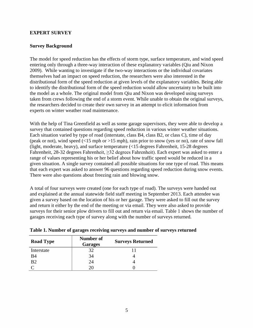
Despite the low response rate, the researchers were still interested in looking at the distribution of the expert responses for specific situations. Since they received the most responses for interstate roads, they began there. Figure 3 shows the speed reductions reported by 11 experts for an interstate road during peak traffic time where there is moderate snowfall and the temperature is between 15 and 28 degrees Fahrenheit. This graph shows a few problems with the data. First, some experts are inconsistent in their answers. For example, expert with ID #9 claims that there will be no speed reduction in this situation unless the wind speed is less than 15 mph and there is rain prior to the snow. This is contradictory to the data and others' experience that higher winds do cause reduction in traffic speed. Another problem is that the responses cover a wide range. This makes it difficult to estimate the effect of a particular covariate on speed reduction due to the large amount of variability between experts. Other situations were examined and the same issues were present. These results led us to question the appropriateness of using survey data to model winter weather performance. We believe that a data driven approach to modeling speed reduction will yield more accurate point estimates and confidence bounds.

6

Figure 3. Speed reduction ranges for 11 experts for interstate roads during peak traffic

times when there is moderate snow fall and the temperature is between 15 and 28 degrees Fahrenheit: two panels have rain prior (bottom) while two do not (top) and two panels

(left) have wind speed greater than 15 mph while two panels (right) have wind speeds less than 15 mph

7

EXPLORATORY ANALYSIS OF SENSOR DATA

Baseline Traffic Trends

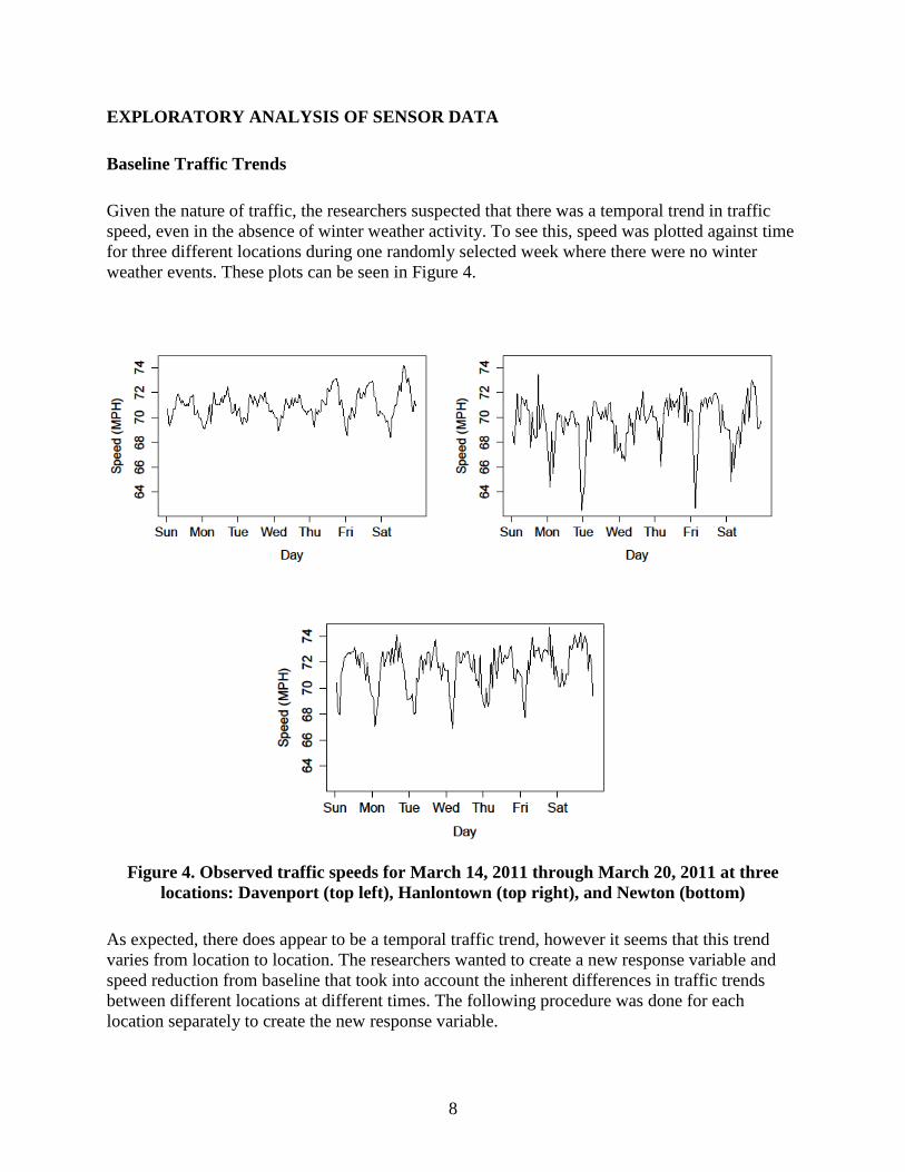
Given the nature of traffic, the researchers suspected that there was a temporal trend in traffic speed, even in the absence of winter weather activity. To see this, speed was plotted against time for three different locations during one randomly selected week where there were no winter weather events. These plots can be seen in Figure 4.

Figure 4. Observed traffic speeds for March 14, 2011 through March 20, 2011 at three

locations: Davenport (top left), Hanlontown (top right), and Newton (bottom)

As expected, there does appear to be a temporal traffic trend, however it seems that this trend varies from location to location. The researchers wanted to create a new response variable and speed reduction from baseline that took into account the inherent differences in traffic trends between different locations at different times. The following procedure was done for each location separately to create the new response variable.

8

1. Select all time points at which storm type was classified as “none" and discard any observations that occurred within 24 hours of the previous storm event.

2. Using the selected observations, calculate the median traffic speed for each hour on each day of the week. These medians are used as the baseline speed for each day/hour combination.

3. For all data points, define speed reduction from baseline as the observed traffic speed subtracted from the baseline traffic speed (i.e. reduction from baseline = baseline-observed).

Variable Exploration and Basic Linear Model

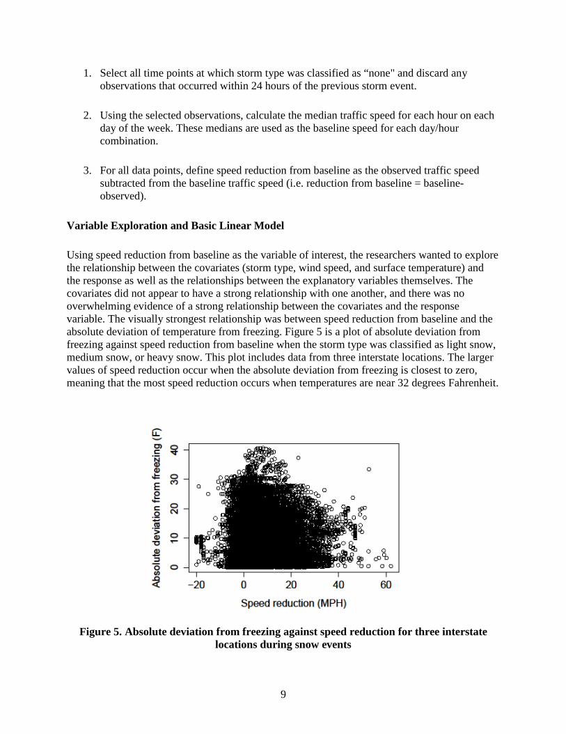
Using speed reduction from baseline as the variable of interest, the researchers wanted to explore the relationship between the covariates (storm type, wind speed, and surface temperature) and the response as well as the relationships between the explanatory variables themselves. The covariates did not appear to have a strong relationship with one another, and there was no overwhelming evidence of a strong relationship between the covariates and the response variable. The visually strongest relationship was between speed reduction from baseline and the absolute deviation of temperature from freezing. Figure 5 is a plot of absolute deviation from freezing against speed reduction from baseline when the storm type was classified as light snow, medium snow, or heavy snow. This plot includes data from three interstate locations. The larger values of speed reduction occur when the absolute deviation from freezing is closest to zero, meaning that the most speed reduction occurs when temperatures are near 32 degrees Fahrenheit.

Figure 5. Absolute deviation from freezing against speed reduction for three interstate

locations during snow events

9

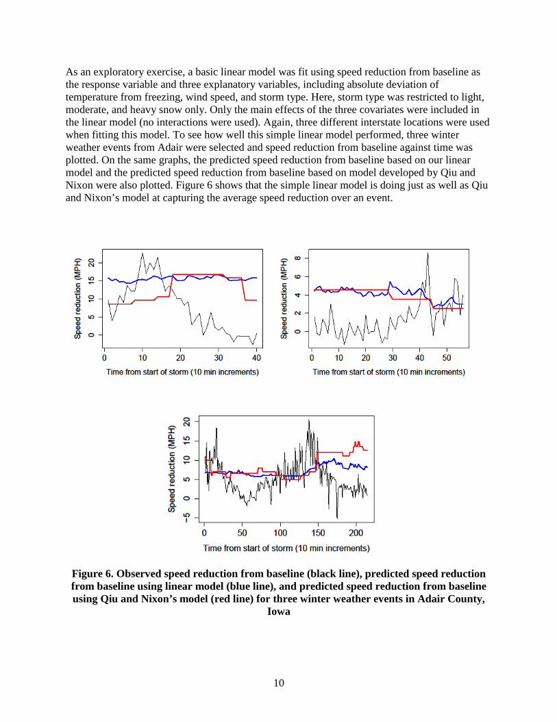
As an exploratory exercise, a basic linear model was fit using speed reduction from baseline as the response variable and three explanatory variables, including absolute deviation of temperature from freezing, wind speed, and storm type. Here, storm type was restricted to light, moderate, and heavy snow only. Only the main effects of the three covariates were included in the linear model (no interactions were used). Again, three different interstate locations were used when fitting this model. To see how well this simple linear model performed, three winter weather events from Adair were selected and speed reduction from baseline against time was plotted. On the same graphs, the predicted speed reduction from baseline based on our linear model and the predicted speed reduction from baseline based on model developed by Qiu and Nixon were also plotted. Figure 6 shows that the simple linear model is doing just as well as Qiu and Nixon’s model at capturing the average speed reduction over an event.

Figure 6. Observed speed reduction from baseline (black line), predicted speed reduction from baseline using linear model (blue line), and predicted speed reduction from baseline using Qiu and Nixon’s model (red line) for three winter weather events in Adair County,

Iowa

10

HIERARCHICAL MODEL FOR ADAIR EVENTS

Format of Data

To develop a hierarchical model for Adair, the researchers used an aggregated form of the data. To get the data in the desired form, they first identified all events, including defining the start of an event as a change in storm type from “none” to a precipitation category and the end of an event as a change in storm type from a precipitation category to “none.” For each event, observations are taken five at a time and the average wind speed, temperature, and speed reduction from baseline are calculated for the groups of five observations. In addition, the most common value of storm type is used for the group of five observations. By aggregating the data in this way, the researchers modeled values that occur every 10 minutes rather than every two minutes. This helped cut down on the influence of individual motorists by ensuring that data from multiple cars was used for each observation.

In addition, a new variable, absolute deviation from freezing, was created. This new variable was calculated by taking the absolute value of the difference between the temperature at time (𝑡𝑡) and 32 degrees Fahrenheit. Based on the evidence presented in the previous section, this new variable was used in place of the raw temperature value as a predictor of speed reduction from baseline.

Nominal Plot Times

In the model, the researchers wanted to account for the impact of snow plows on road conditions and thus speed reduction. According to the garage manager in Adair, it is estimated that a plow first passes the sensor 30 minutes after a storm begins and returns every 60 minutes. Since the data is aggregated over 10 minutes, this means that the plow returns after six observations.

Model Formulation

Consider one storm event for Adair. Let {𝑌𝑌𝑡𝑡: 𝑡𝑡 = 1,2, … ,𝑇𝑇} denote the recorded speed reduction from baseline at time (𝑡𝑡). The model for 𝑌𝑌𝑡𝑡 is as follows.

𝑌𝑌𝑡𝑡 = ℎ(𝜷𝜷,𝒙𝒙𝒕𝒕) + 𝑤𝑤𝑡𝑡

𝑤𝑤𝑡𝑡 = 𝛾𝛾𝑤𝑤𝑡𝑡−1 + 𝑣𝑣𝑡𝑡

where 𝑤𝑤0 = 0 and 𝑣𝑣𝑡𝑡 are independent identically distributed random variables following a normal distribution with a mean of 0 and a variance of 𝜏𝜏2. Define

ℎ∗(𝜷𝜷,𝒙𝒙𝒕𝒕) = 𝛽𝛽𝑜𝑜𝑋𝑋𝑡𝑡,𝑁𝑁𝑜𝑜𝑁𝑁𝑁𝑁𝑜𝑜𝑁𝑁 + 𝛽𝛽1𝑋𝑋𝑡𝑡,|𝑡𝑡𝑡𝑡𝑡𝑡𝑡𝑡−32| + 𝛽𝛽2𝑋𝑋𝑡𝑡,𝐿𝐿𝐿𝐿𝐿𝐿ℎ𝑡𝑡𝑁𝑁𝑁𝑁𝑜𝑜𝑁𝑁 + 𝛽𝛽3𝑋𝑋𝑡𝑡,𝑀𝑀𝑜𝑜𝑀𝑀𝑁𝑁𝑁𝑁𝑜𝑜𝑁𝑁+ 𝛽𝛽4𝑋𝑋𝑡𝑡,𝐻𝐻𝑡𝑡𝑎𝑎𝑎𝑎𝑎𝑎𝑁𝑁𝑁𝑁𝑜𝑜𝑁𝑁 + 𝛽𝛽5𝑋𝑋𝑡𝑡,𝑁𝑁𝐿𝐿𝑁𝑁𝑀𝑀

11

Then,

ℎ(𝜷𝜷,𝒙𝒙𝒕𝒕) =

⎩⎪⎨

⎪⎧

ℎ∗(𝜷𝜷,𝒙𝒙𝒕𝒕), 𝑡𝑡 ≤ 4ℎ∗(𝜷𝜷,𝒙𝒙𝒕𝒕) + 𝜆𝜆(4 − 𝑡𝑡), 4 < 𝑡𝑡 ≤ 10ℎ∗(𝜷𝜷,𝒙𝒙𝒕𝒕) + 𝜆𝜆(10 − 𝑡𝑡), 10 < 𝑡𝑡 ≤ 16ℎ∗(𝜷𝜷,𝒙𝒙𝒕𝒕) + 𝜆𝜆(16 − 𝑡𝑡), 16 < 𝑡𝑡 ≤ 22

⋮ ⋮

ℎ(𝜷𝜷,𝒙𝒙𝒕𝒕) is comprised of two pieces. The first piece, ℎ∗(𝜷𝜷,𝒙𝒙𝒕𝒕), is a linear combination of weather covariates. The second piece takes into account the impact of snow plows on speed reduction, represented here by the parameter λ.

A Bayesian analysis via Markov Chain Monte Carlo methods was performed, thus the researchers needed to place prior distributions on 𝛽𝛽𝐿𝐿 (𝑖𝑖 = 1,2, … ,5), λ, γ, and 𝜏𝜏2. The following non-informative priors were used.

𝛽𝛽𝐿𝐿~𝑁𝑁�0,𝜎𝜎𝛽𝛽𝑖𝑖2 = 100�

𝜆𝜆~𝑁𝑁�0,𝜎𝜎𝜆𝜆2 = 100�

𝛾𝛾~𝑈𝑈𝑈𝑈𝑖𝑖𝑈𝑈(−1,1)

𝜏𝜏2~𝐼𝐼𝐼𝐼(0.01, 0.01)

Implementation of the Model

A Metropolis within Gibbs sampler was written to simulate values from the posterior distribution of the parameters. These parameters were then used to estimate the speed reduction from baseline based on the research model. To ensure that the model was working correctly, the researchers simulated data (so the true parameter values were known) and fit the model to estimate the parameter values. For all parameters, the estimates were nearly identical to the true values.

Afterwards, they moved on to fitting the model to a winter weather event from Adair County in Iowa. This particular event began on January 9, 2011 at 10:31 a.m. and ended on January 10, 2011 at 11:49 p.m. The precipitation type was initially light snow, but transitioned to medium snow approximately one-third of the way into the event. Figure 7 shows the observed traffic speed and the fitted model with 90 percent prediction bands. The width of the prediction bands tells shows that the model is doing a good job capturing the variability that is present in the data.

12

Figure 7. Model fitted to snow event in Adair County where x-axis represents 10 minute

intervals starting at 10:31 a.m. on January 9, 2011 and ending at 11:49 p.m. on January 10, 2011 and blue dotted lines are 90 percent error bounds

Table 2 gives the estimates of the parameter values along with a 90 percent interval based on 50,000 observations drawn from the posterior distribution after a burn-in of 2,000 observations. These estimates and intervals show that the temperature, as the absolute deviation from freezing, has a definite impact on traffic speed reduction from baseline. This is in contrast to wind, which does not seem to have much of an effect on speed reduction. Looking at the parameter λ, there is evidence that the snow plows have an effect on traffic speed. Finally, the researchers noted that they did not have good parameter estimates for 𝛽𝛽0 and 𝛽𝛽4 (i.e. the parameters corresponding to “no snow” and “heavy snow,” respectively). This is to be expected since, in this particular event, there was only “light snow” and “medium snow,” so the information they had about 𝛽𝛽0 and 𝛽𝛽4 comes solely from the prior distributions.

13

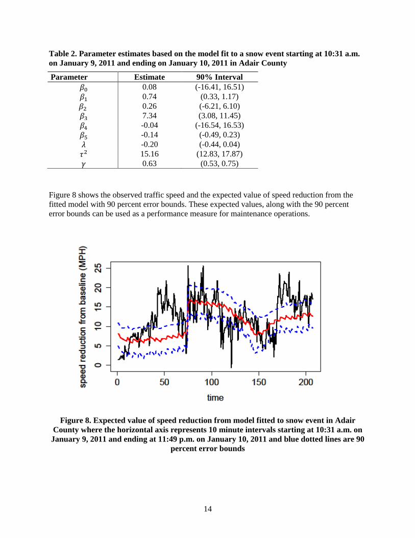
Table 2. Parameter estimates based on the model fit to a snow event starting at 10:31 a.m. on January 9, 2011 and ending on January 10, 2011 in Adair County

Parameter Estimate 90% Interval 𝛽𝛽0 0.08 (-16.41, 16.51) 𝛽𝛽1 0.74 (0.33, 1.17) 𝛽𝛽2 0.26 (-6.21, 6.10) 𝛽𝛽3 7.34 (3.08, 11.45) 𝛽𝛽4 -0.04 (-16.54, 16.53) 𝛽𝛽5 -0.14 (-0.49, 0.23) 𝜆𝜆 -0.20 (-0.44, 0.04) 𝜏𝜏2 15.16 (12.83, 17.87) 𝛾𝛾 0.63 (0.53, 0.75)

Figure 8 shows the observed traffic speed and the expected value of speed reduction from the fitted model with 90 percent error bounds. These expected values, along with the 90 percent error bounds can be used as a performance measure for maintenance operations.

Figure 8. Expected value of speed reduction from model fitted to snow event in Adair

County where the horizontal axis represents 10 minute intervals starting at 10:31 a.m. on January 9, 2011 and ending at 11:49 p.m. on January 10, 2011 and blue dotted lines are 90

percent error bounds

14

POTENTIAL DIRECTIONS AND FUTURE WORK

The researchers developed a hierarchical model that takes into account the effect of winter weather covariates as well as maintenance operations on speed reduction during snow events in Adair County, Iowa. This model proved to do a good job predicting the speed reduction from the baseline over time as well as in capturing the variability in the data. Future work needs to be done to achieve the goal of using this model as a performance measurement tool. Namely, a third level in the hierarchical model needs to be added to allow for estimation of the distributions of the parameter values across all events for a given location. Once these parameter distributions are estimated, performance as a storm event is occurring can be better assessed. Also, the effect of certain covariates on traffic speeds across multiple locations can then be compared.

15

REFERENCES

Greenfield, Tina, Matt Haubrich, Mark Kaiser, Jing Li, Zhengyuan Zhu, and Daniel Fortin. Winter Performance Measurement Using Traffic Speed Modeling. Iowa Highway Research Board, Iowa Department of Transportation, 2011.

Qiu, Linn and Wilfred Nixon. Performance Measurement for Highway Winter Maintenance Operations. IIHR Report 474. Iowa Highway Research Board, 2009.

17