1MG Level 1 PRECALCULUS Theory Lycée Denis-de-Rougemont 2006-2007
- 1 - YAy & PRi
TABLE OF CONTENTS
§0 VOCABULARY ________________________________________ - 5 -
§1 NUMBERS ___________________________________________ - 7 -
1.1 Sets of numbers ___________________________________________ - 7 -
1.2 Reminder : Exponents and products__________________________ - 9 -
1.3 The real number line______________________________________ - 10 -
1.4 Intervals ________________________________________________ - 10 -
§2 ABSOLUTE VALUE ___________________________________ - 11 -
§3 SYSTÈMS OF ÉQUATIONS ______________________________ - 11 -
3.0 2x2 systems______________________________________________ - 11 -
3.1 3x3 systems______________________________________________ - 13 -
§4 THE STRAIGHT LINE__________________________________ - 14 -
4.0 Generalities _____________________________________________ - 14 -
4.1 Gradient or slope of a line _________________________________ - 14 -
4.2 Vertical shift and intersections with the axes _________________ - 15 -
4.3 Types of lines____________________________________________ - 15 -
4.4 Remarks ________________________________________________ - 15 -
4.5 Equation of a line ________________________________________ - 16 -
§5 QUADRATICS _______________________________________ - 17 -
5.0 Definition and properties__________________________________ - 17 -
5.1 Solving quadratic expressions ______________________________ - 20 -
5.2 Factorisation ____________________________________________ - 21 -
§6 SOLVING EQUATIONS _________________________________ - 22 -
6.0 Equations which reduce to quadratics equations ______________ - 22 -
6.1 Irrational equations_______________________________________ - 23 -
6.2 Rational equations _______________________________________ - 23 -
6.3 Equations involving an absolute value_______________________ - 24 -
6.4 Inequalities______________________________________________ - 25 -
6.5 Systems of inequalities ____________________________________ - 26 -

1MG Level 1 PRECALCULUS Theory Lycée Denis-de-Rougemont 2006-2007
- 2 - YAy & PRi
§7 APPLICATIONS AND FUNCTIONS_________________________ - 27 -
7.0 Applications_____________________________________________ - 27 -
7.1 Functions _______________________________________________ - 28 -
7.2 Inverse function__________________________________________ - 31 -
7.3 Composite function_______________________________________ - 33 -
§8 POLYNOMIALS ______________________________________ - 34 -
8.0 Reminder _______________________________________________ - 34 -
8.1 Addition and subtraction __________________________________ - 34 -
8.2 Multiplication ___________________________________________ - 35 -
8.3 Long Division ___________________________________________ - 35 -
§9 EXPONENTIAL AND LOGARITHMIC FUNCTIONS _____________ - 38 -
9.0 Definition and properties__________________________________ - 38 -

1MG Level 1 PRECALCULUS Theory Lycée Denis-de-Rougemont 2006-2007
- 3 - YAy & PRi
INTRODUCTION AND HISTORY
Mathematics (colloquially, maths or math) is the body of knowledge centered on
concepts such as quantity, structure, space, and change. It evolved, through the use of
abstraction and logical reasoning, from counting, calculation, measurement, and the
study of the shapes and motions of physical objects. Mathematicians explore such
concepts, aiming to formulate new conjectures and establish their truth by rigorous
deduction from appropriately chosen axioms and definitions.
Knowledge and use of basic mathematics
have always been an inherent and integral
part of individual and group life.
Refinements of the basic ideas are visible
in ancient mathematical texts originating in
ancient Egypt, Mesopotamia, Ancient
India, and Ancient China with increased
rigour later introduced by the ancient
Greeks. From this point on, the
development continued in short bursts
until the Renaissance period of the 16th
century where mathematical innovations
interacted with new scientific discoveries leading to an acceleration in understanding
that continues to the present day.
Today, mathematics is used throughout the world in many fields, including science,
engineering, medicine and economics. The application of mathematics to such fields,
often dubbed applied mathematics, inspires and makes use of new mathematical
discoveries and has sometimes led to the development of entirely new disciplines.
Mathematicians also engage in pure mathematics for its own sake without having any
practical application in mind, although applications for what begins as pure
mathematics are often discovered later on.
Euclid, Greek mathematician, 3rd century BC, known today as the father of geometry; shown here in a detail of The School of Athens by Raphael.
1MG Level 1 PRECALCULUS Theory Lycée Denis-de-Rougemont 2006-2007
- 4 - YAy & PRi
The evolution of mathematics might be seen to be an ever-increasing series of
abstractions, or alternatively an expansion of subject matter. The first abstraction was
probably that of numbers. The realization that two apples and two oranges have
something in common was a breakthrough in human thought. In addition to recognizing
how to count physical objects, prehistoric peoples also recognized how to count
abstract quantities, like time days, seasons, years. Arithmetic that is to say addition,
subtraction, multiplication and division, naturally followed. Monolithic monuments testify
to knowledge of geometry.
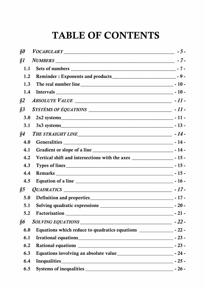
Further steps need writing or some other system for
recording numbers such as tallies or the knotted strings
called quipu used by the Inca Empire to store numerical
data. Numeral systems have been many and diverse.
From the beginnings of recorded history, the major
disciplines within mathematics arose out of the need to
do calculations relating to taxation and commerce, to
understand the relationships among numbers, to
measure land, and to predict astronomical events.
These needs can be roughly related to the broad
subdivision of mathematics, into the studies of quantity,
structure, space, and change.
Mathematics since has been much extended, and there has been a fruitful interaction
between mathematics and science, to the benefit of both. Mathematical discoveries
have been made throughout history and continue to be made today.
A quipu, a counting device used by the Inca.
1MG Level 1 PRECALCULUS Theory Lycée Denis-de-Rougemont 2006-2007
- 5 - YAy & PRi
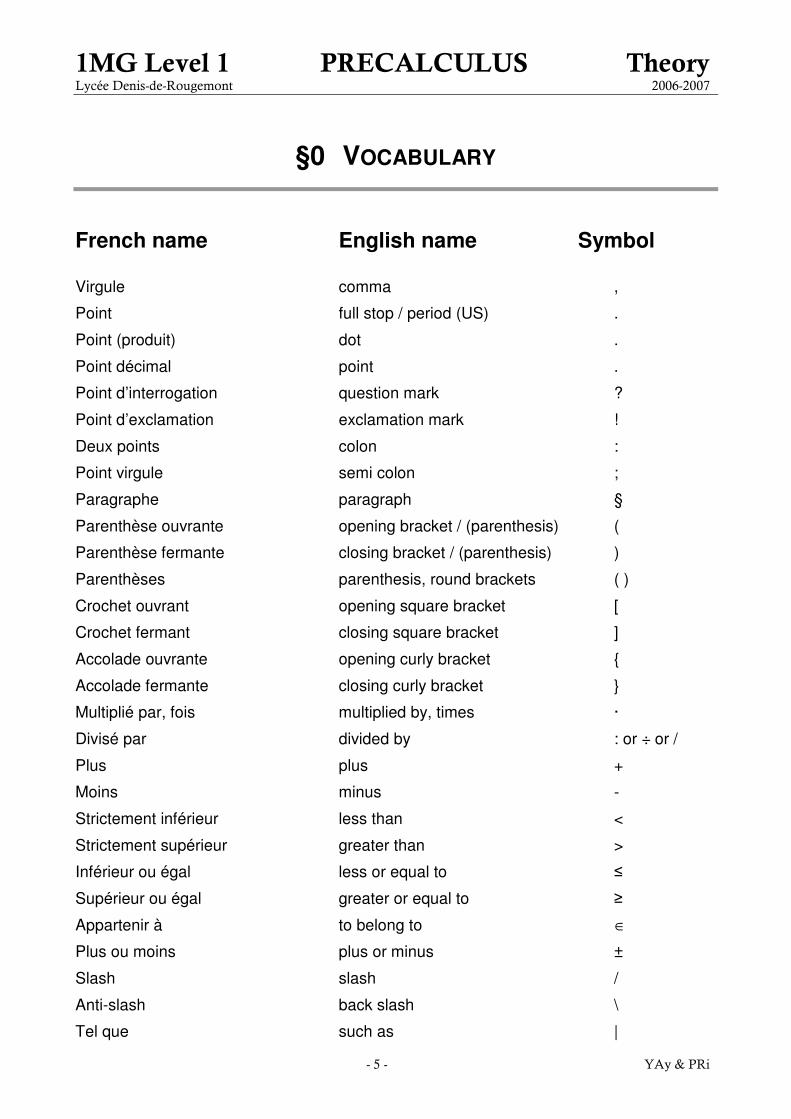
§0 VOCABULARY
French name English name Symbol
Virgule comma ,
Point full stop / period (US) .
Point (produit) dot .
Point décimal point .
Point d’interrogation question mark ?
Point d’exclamation exclamation mark !
Deux points colon :
Point virgule semi colon ;
Paragraphe paragraph §
Parenthèse ouvrante opening bracket / (parenthesis) (
Parenthèse fermante closing bracket / (parenthesis) )
Parenthèses parenthesis, round brackets ( )
Crochet ouvrant opening square bracket [
Crochet fermant closing square bracket ]
Accolade ouvrante opening curly bracket {
Accolade fermante closing curly bracket }
Multiplié par, fois multiplied by, times ·
Divisé par divided by : or ÷ or /
Plus plus +
Moins minus -
Strictement inférieur less than <
Strictement supérieur greater than >
Inférieur ou égal less or equal to ≤
Supérieur ou égal greater or equal to ≥
Appartenir à to belong to ∈
Plus ou moins plus or minus ±
Slash slash /
Anti-slash back slash \
Tel que such as |

1MG Level 1 PRECALCULUS Theory Lycée Denis-de-Rougemont 2006-2007
- 6 - YAy & PRi
Ensemble set
Résoudre to solve
Idem ditto "
Etoile star *
Droite (straight) line
Pontillé dotted
Axe axis
Axes axes
Echelle (graphe) scale
Premier (nombre) prime (number)
Carré square
Au carré squared
Additionner to add (up)
Noter to note (down) / to write down
Règle (loi) rule
Diviseur factor, divisor
Exposant exponent, index (plural indices)
Pair even
Impair odd
Calcul calculation
Calculer to calculate, to compute
Dessiner (graphe) to draw, to plot
Esquisser to sketch
Chiffre digit

1MG Level 1 PRECALCULUS Theory Lycée Denis-de-Rougemont 2006-2007
- 7 - YAy & PRi
§1 NUMBERS
1.1 Sets of numbers
When we want to treat a collection of similar but distinct objects as a whole, we use the
idea of a set (ensemble). For example, the set of digits consists of the collection of
numbers 0, 1, 2, 3, 4, 5, 6, 7, 8 and 9. If we use the symbol D to denote the set of digits,
then we can write :
{ } { }Read as "set of all such that is a digit"
0, 1, 2, 3, 4, 5, 6, 7, 8, 9 is a digit
x x
D x x= =���������
Natural numbers : { }0 ; 1 ; 2 ; 3 ; 4 ; ...=�
Integer numbers : { }... ; 2 ; 1 ; 0 ; 1 ; 2 ; ...= − −�
Rational numbers : ; , , 0p
p q qq
= ∈ ∈ ≠
� � �
Real numbers : �
Complex numbers : 2( 1)i = −
Diagram of Venn
Definition
A positive integer p is a prime number (nombre premier) or prime if p ≠ 1 and if its only
positive divisors are 1 and itself.
� � � �
1
4
1097
12
4
-4
-876
0
2
π−
7
3 8−
1,33
5−
3π
54
2
−
984
13
−
1,764
45
7 1,4−1
2
4
« such that »

1MG Level 1 PRECALCULUS Theory Lycée Denis-de-Rougemont 2006-2007
- 8 - YAy & PRi
Remark
A set of numbers with a « * » is a set without 0.
Thus, { }* 1 ; 2 ; 3 ; 4 ; ...=� , { }* ... ; 2 ; 1 ; 1 ; 2 ; ...= − −� , …
The empty set is denoted by the symbol { } or ∅ .
Generally, when we consider two sets A and B they are formed of elements of a certain
set U called universal set (univers).
Definitions
1) A set A is included in a set B if every element of A belongs to B. We say that A
is a subset (sous-ensemble) of B. We note it BA ⊂ .
Examples
⊂� �
{ } { }; ; ; ;a e i o u alphabet⊂
2) Intersection : { }A B x x A x B∩ = ∈ ∈and
Examples
{ } { } { }1 ; 2 ; 3 2 ; 0 ; 1 ; 3 ; 5 1 ; 3∩ − =
{ } { } { }; ; ; ;red green blue white green yellow green∩ =
3) Union : { }A B x x A x B∪ = ∈ ∈or
Examples
{ } { } { }1 ; 2 ; 3 0 ; 1 ; 3 ; 5 0 ; 1 ; 2 ; 3 ; 5∪ =
{ } { }
{ }
; ; ;
; ; ;
red green white green yellow
red white green yellow
∪ =
=
4) Difference : A \ B { }x x A x B= ∈ ∉and
Examples
{ } { } { }0 ; 1 ; 3 ; 5 \ 1 ; 2 ; 3 0 ; 5=
{ } { }
{ }
; ; \ ; ;
;
red green blue white green yellow
red blue
=
=
B
A
U
B A
U
B A
U
B A
U

1MG Level 1 PRECALCULUS Theory Lycée Denis-de-Rougemont 2006-2007
- 9 - YAy & PRi
5) Complement : A
UA C= = U \ A
Example
{ } { }
{ }
0 ; 1 ; 2 ; 3 ; 4 ; 5 ; 6 1 ; 2 ; 3
0 ; 4 ; 5 ; 6
U A
A
= =
=
1.2 Reminder : Exponents and products
Integer exponents provide a shorthand device for representing repeated multiplications of
a real number a :
factors
...n
n
a a a a= ⋅ ⋅ ⋅�����
where a is called the base and n the exponent or power. We read an as “a raised to the
power n” or as “a to the nth power” and shortly as “a power n”.
We define that :
if 0a ≠ then 0 1a =
if 0a ≠ and n a positive integer then 1n
na
a
−=
if *n ∈� then 1
nna a=
Rules of indices
m nm n aa a+
⋅ = The multiplication rule
m nm n aa a−
÷ = The division rule
)(m n m naa
⋅= The power-on-power rule
( )m m ma b a b⋅ = ⋅ The factor rule
Example
It is possible to combine all these rules : 7 2 3 21 6 3(5 ) 125a r p a r p=
Some important products
1) ( )a b c ab ac⋅ + = + distributivity of the multiplication over the addition
2) If 0ab = than either 0a = , 0b = or 0a b= =
3) 2 2 2( ) 2a b a ab b+ = + + Example 2 2( 5) 10 25x x x+ = + +
4) 2 2 2( ) 2a b a ab b− = − + Example 2 2( 5) 10 25x x x− = − +
5) 2 2( )( )a b a b a b+ − = − Example 2( 5)( 5) 25x x x+ − = −
A
U

1MG Level 1 PRECALCULUS Theory Lycée Denis-de-Rougemont 2006-2007
- 10 - YAy & PRi
1.3 The real number line
The real numbers can be represented by points on a line called real number line (axe des
reels). Every real number corresponds to a point of the line and each point of the line has
a unique real number associated with it.
The point of the line which is associated with the real number 0 is called the origin and is
noted O. The point 1 unit to the right of O corresponds to the number 1, etc. Notice that an
arrowhead on the right end of the line indicates the direction in which the numbers
increase.
1.4 Intervals
A set containing all real numbers between two given endpoints is called interval.
If a and b are two real number such that a < b, we note :
[ ] { }; anda b x x a x b= ∈ ≤ ≤� closed interval
] [ { }; anda b x x a x b= ∈ < <� open interval
[ [ { }; anda b x x a x b= ∈ ≤ <�
] ] { }; anda b x x a x b= ∈ < ≤�
a and b are called endpoints (bornes) of the interval.
Example ] ] { }1 ; 5 and 1 5x x x= ∈ < ≤�
It is possible to represent an interval on the real number line. For that we place the two
endpoints and we use bold type if the endpoint belongs to the interval. Finally, we thick the
part of the line that corresponds to the interval we have to draw.
Example
Represent, on the real number line, the interval ] ]1 ; 5 .
O
1 5
O 2 3 -1 1 -2 -3 -4 4
0,5 2 -0,5 π �
… …

1MG Level 1 PRECALCULUS Theory Lycée Denis-de-Rougemont 2006-2007
- 11 - YAy & PRi
§2 ABSOLUTE VALUE
The absolute value or modulus of x, denoted by the symbol x , is defined by :
if 0
if 0
x xx
x x
≥=
− <
Examples 5 5= 5 ( 5) 5− = − − =
§3 SYSTEMS OF EQUATIONS
3.0 2x2 systems
When we solve such a system, we look for x and y that satisfy both equations. Actually we
search the intersection point of two lines. For that we have 3 different methods : addition,
substitution and graphic. We are going to see these 3 methods with an example.
We consider the following system : 5 2 5 (1)
3 2 (2)
x y
x y
− =
− =
1) ADDITION
The goal is to have the same quantity of x or y in both equations but with the
opposite sign. For that, we multiply the equation (2) by –2 and we obtain :
5x – 2y = 5
–6x + 2y = –4 ⊕
–x = 1 ⇒ x = –1
We replace x in the equation (2) to find y : 3·(–1) – y = 2 ⇒ y = – 5

1MG Level 1 PRECALCULUS Theory Lycée Denis-de-Rougemont 2006-2007
- 12 - YAy & PRi
2) SUBSTITUTION
The purpose is to express x in terms of y or y in terms of x.
We modify the equation (2) to have : y = 3x – 2 (3)
Then we replace y in the equation (1) by the expression (3) to obtain :
5x – 2(3x – 2) = 5
5x – 6x + 4 = 5
–x = 1 ⇒ x = –1
We replace x by –1 in the equation (3) to find y : y = 3·(–1) – 2 ⇒ y = – 5
3) GRAPHIC
The objective is to draw the two lines and the intersection gives us the
solution. The first thing to do is to express y in terms of x and then to draw the
lines :
(1) becomes y = 2
55 −x and (2) becomes y = 3x – 2
This method is not often used. Actually it is relatively long and not really
precise because if the coordinates of the intersection point are not integer
numbers, it is very difficult and even impossible to determine them precisely.
Remarks
1) Two equations multiple of each other are said to be equivalent. Consequently, the
system has an infinite number of solutions.
2) If the system has no solutions (the resolution gives us an impossible result) then the
equations are said to be incompatible.
Example Solve
=−
−=+−−
432
23)12(2
1
yx
yx
( 2) 1 ( 1)12 1 6 4 2 6 5(2 1) 3 2
22 3 4 2 3 4
2 3 4
13 1
3
1 3We replace in the second equation to find : 2 3 4
3 2
andx y x yx y
x y x yx y
y y
y x x x
⋅ − + ⋅ −− − − = − + = −− + = − ⇒ ⇒ ⊕ − = − = − =
= − ⇒ = −
− ⋅ − = ⇒ =

1MG Level 1 PRECALCULUS Theory Lycée Denis-de-Rougemont 2006-2007
- 13 - YAy & PRi
3.1 3x3 systems
To solve a 3x3 system, we eliminate one of the variables using twice the addition or
substitution method. In other words, we eliminate the variable we choose thanks to two
equations of the system. Then we repeat the operation using the last equation we haven’t
used until now. Thus we obtain a 2x2 system that we solve as in 3.0. Let’s illustrate this
with an example. We consider the following system :
−=+−
−=−−−
=−−
)3(20435
)2(12
)1(722
zyx
zyx
zyx
We add the equations (1) and (2) to eliminate x :
(1) 2 2 7
(2) 2 1
(4) 2 3 6
x y z
x y z
y z
− − =⊕
− − − = −
− − =
We eliminate one more time x but with equations (2) and (3) :
2 1(2) 5
5 3 4 20(3) 2
10 5 5 5
10 6 8 40
(5 ) 11 3 45
x y z
x y z
x y z
x y z
y z
− − − = − ⋅
− + = − ⋅
− − − = −⊕
− + = −
− + = −
We have now a 2x2 system, formed of equations (4) and (5), to solve :
2 3 6(4 )
11 3 45(5)
13 39 3
y z
y z
y y
− − =⊕
− + = −
− = − ⇒ =
We find z by replacing 3y = in the equation (5) : 11 3 3 45 4z z− ⋅ + = − ⇒ = −
Finally, we find the value of x by replacing 3y = and 4z = − in one of the equations (1),
(2), or (3) : 2 3 2 ( 4) 7 1x x− − ⋅ − = ⇒ = .

1MG Level 1 PRECALCULUS Theory Lycée Denis-de-Rougemont 2006-2007
- 14 - YAy & PRi
line
§4 THE STRAIGHT LINE
4.0 Generalities
The degree of a function f is one if it can be written in the form : y = ax + b ( ,a b ∈ � )
The graph of such a function is a straight line (droite). The coordinates of its points are :
(x ; y). It is very important to notice that for a chosen x the y-coordinate is given by the
function evaluated at x, consequently y = f(x) and the coordinates of the points become :
(x ; f(x)).
The coefficients a and b represent : a : the gradient or slope (pente) of the line
b : the y-intercept of the line
4.1 Gradient or slope of a line
By definition, the gradient is the ratio y
ax
∆=
∆,
where x∆ is the increase in the x-coordinate and
y∆ is the corresponding increase in the y-coordinate.
To find the gradient, you choose any two points lying on the line : );( AA yxA and );( BB yxB .
Then you compute x∆ = the x-step = AB xx − and y∆ = the y-step = AB yy − . Finally, the
gradient is :
B A
B A
y yya
x x x
−∆= =
∆ −
This result does not depend on the point A and B you have selected.
Example
Calculate the gradient a of the line joining (6 ; 9) and ( – 4 ; 12 ).
12 9 3
0,34 6 10
a−
= = = −− − −
x∆
y∆

1MG Level 1 PRECALCULUS Theory Lycée Denis-de-Rougemont 2006-2007
- 15 - YAy & PRi
4.2 Vertical shift and intersections with the axes
The constant b of the equation of a line represents the vertical shift (décalage vertical) of
the line. It corresponds to the y-coordinate of the intersection point between the line
and the y-axis. Consequently, to find the coordinates of this point we have to replace x by
zero in the equation of the line. We obtain y = b and the coordinates of this point are (0 ; b).
The intersection point between the line and the x-axis is given by the resolution of the
equation : 0 = ax + b because every point on the x-axis has a y-coordinate equals to zero.
The coordinates of this point are (x ; 0).
Vocabulary
The x-coordinate of a point is also called abscissa and the y-coordinate ordinate.
4.3 Types of lines
Depending on the value of the coefficients a and b, the line is :
Linear if 0 and 0a b≠ = : passes through the origin O(0 ; 0).
Constant if 0 anda b= ∈� : parallel to the x-axis.
Affine if , 0a b ≠ : not horizontal, shifted vertically of b over the origin.
Examples
63)(1 −= xxf is affine, xxf 6,4)(2 −= is linear, 8,12)(3 =xf is constant.
4.4 Remarks
1) The sign of the gradient determines if the line increases or decreases (rises or falls).
2) Two parallel lines have the same gradient.
3) Two lines with gradient m1 and m2 are perpendicular if m1·m2 = –1
4) To draw a line :
a) Place a first point thanks to the y-intercept (0 ; b). Then, from that point, draw
the gradient (move of x-step to the right and move up or down of y-step) or…
b) Place a first point thanks to the y-intercept (0 ; b). Then find a second point
thanks to the equation of the line.

1MG Level 1 PRECALCULUS Theory Lycée Denis-de-Rougemont 2006-2007
- 16 - YAy & PRi
4.5 Equation of a line
To determine the equation of a line means to determine the value of the constants a and b.
For that we have two different ways to proceed :
a) Use two points on the line to calculate the gradient. Then find the y-intercept by
substituting the coordinates of one of your two points in the equation y ax b= + , of
which only b is now unknown. Solve this equation to obtain b or…
b) Use two points of the line and replace x and y of the line by the coordinates x and
y of one of your two points. Ditto with the second point. Now you have to solve a
2x2 system.
Examples
1) The two following lines are parallel : f(x) = 3x + 4 and f(x) = 3x – 5
2) The two following lines are perpendicular : f(x) = 2x – 1 and f(x) = x2
1− + 3
3) Find the equation of the line that passes through A(–2 ; 3) and B(4 ; –5) :
a) The general equation of a line is y = ax + b and we have to find a and b. The
gradient is 5 3 8 4
4 ( 2) 6 3
ya
x
∆ − − − −= = = =
∆ − −, so
4
3y x b
−= + . To determine b we
substitute x and y of the line by the coordinates x and y of the point A :
4
3 ( 2)3
b−
= ⋅ − + ⇒ 1
3b = and finally,
4 1
3 3y x
−= + .
b) We substitute x and y of the line by the coordinates x and y of the points A
and B :
3 2 4 1
and 3 35 4
a ba b
a b
= − + −⇒ = =
− = + so y =
3
4−x +
3
1.

1MG Level 1 PRECALCULUS Theory Lycée Denis-de-Rougemont 2006-2007
- 17 - YAy & PRi
−3 −2 −1 1 2 3
2
4
6
8
10
−2 −1 1 2 3 4
2
4
6
8
10
−2 −1 1 2 3 4
−2
2
4
6
8
−5 −4 −3 −2 −1 1
−6
−4
−2
2
4
§5 Quadratics
5.0 Definition and properties
A quadratic function is s function defined by a second-degree polynomial in one variable.
Thus it is a function of the form :
2( )f x ax bx c= + +
where a, b, c are real numbers and a ≠ 0. The graph of such a function is a parabola.
Examples
y = x2 y = (x – 1)2
y = (x – 1)2 – 2 y = – (x + 2)2 + 3

1MG Level 1 PRECALCULUS Theory Lycée Denis-de-Rougemont 2006-2007
- 18 - YAy & PRi
We can prove that :
2 22 4
2 4
b b acax bx c a x
a a
− + + = + −
. Consequently, any quadratic
function can be written as 2( ) ( )f x a x h k= − + where 2
bh
a= − and
2 4
4
b ack
a
−= − . Its graph
is a parabola whose vertex is V(h ; k). As ( )y f x= we have that ( )k f h= and V(h ; f(h)). The
axis of symmetry is the vertical line with equation b
x2a
= −= −= −= − .
Remarks
1. If a > 0 then the parabola opens up (smile).
If a < 0 then the parabola opens down (grimace).
2. The process of writing 2( )f x ax bx c= + + as 2( ) ( )f x a x h k= − + is called
« completing the square » and the form 2( ) ( )f x a x h k= − + is called
« completed square form » (« forme du sommet »).
3. The point where a parabola meets its axis of symmetry is called the vertex
(sommet).
4. If a is positive, the vertex is at the lowest point of the graph (minimum); if a is
negative the vertex is at the highest point (maximum).
5. Suppose that you have two functions y = f(x) and y = g(x). The coordinates (xi , yi)
of the intersection point satisfy both graphs. Therefore, to find the intersection
point of two functions we have to solve the equation f(x) = g(x). After having found
x, don’t forget to calculate y.
2( ) with y a x h k= − + a < 0 2( ) with y a x h k= − + a > 0
k
h
V
k
h
V

1MG Level 1 PRECALCULUS Theory Lycée Denis-de-Rougemont 2006-2007
- 19 - YAy & PRi
Examples
1. Find the completed square form of the parabola 2( ) 10 32f x x x= + + .
METHOD 1
First of all we consider only the terms with x and we want to form (x – h)2.
In this example we need to write x2 + 10x as (x – h)2. If we develop (x – h)2 we
obtain x2 – 2hx + h2. As we have 2h = 10 and we want h, we have to divide the
coefficient in front of x, which is 10, by 2 so we have (x + 5)2. But if we develop it,
we obtain :
(x + 5)2 = x2 + 10x + 25
that is not exactly x2 + 10x. Therefore, we have to subtract 25 from the
parenthesis and we obtain (x + 5)2 – 25 = x2 + 10x. Finally we have to add 32 on
both sides to have the equation of our example which is x2 + 10x + 32 :
x2 + 10x = (x + 5)2 – 25
x2 + 10x +32 = (x + 5)2 – 25 + 32
x2 + 10x + 32 = (x + 5)2 + 7
METHOD 2
We use the formula 10
52 2
bh
a= − = − = − . We replace this value in the parentesis
so (x – (-5))2 = (x + 5)2. As in method 1 we don’t exactly have x2 + 10x, but
x2 + 10x + 25 so we have to subtract 25 to the parenthesis and then add 32 to
have the given quadratic.
2. Find the vertex and the axis of symmetry of the parabola 2 2 15y x x= + − .
METHODE 1 2
Axis of symmetry : 1 12 2
: It is on the axis of symmetry therefore the -coordinate is 1.
To find the -coordinate, we replace 1 in the equation of the parabola :
Vertex
bx x
a
x
y x
− −= = = − ⇒ = −
−
= −
1 2 15 16 and ( 1; 16 )y V= − − = − − −
METHODE 2
2 2
2 2
We write the equation into ( ) .
( 1) 1 15 ( 1) 16 thus the vertex is ( 1 ; 16 )
y ax bx c y a x h k
y x x V
= + + = − +
= + − − = + − − −
METHODE 3 Cf exercise 25

1MG Level 1 PRECALCULUS Theory Lycée Denis-de-Rougemont 2006-2007
- 20 - YAy & PRi
5.1 Solving quadratic expressions
When we search the intersection of f(x) = ax2 + bx + c with the x-axis we have to solve the
equation ax2 + bx + c = 0, where a, b and c are constants. The solution(s) of ax2+ bx + c = 0,
where 0a ≠ , is (are) given by the fomula :
2
1,2
4
2
b b acx
a
− ± −= Viète
Remark
The solutions of ax2+ bx + c = 0 are called zeros or roots.
Demonstration
We have seen that we can write :
2 22 4
2 4
b b acax bx c a x
a a
− + + = + −
We look for the solution(s) of ax2 + bx + c = 0 :
2 2 22 2
2
2 2 22
1,2
22
2
4 4 40 ( ) ( )
2 4 2 24
4 4 4( )
2 4 2 2 2
4( )
2 4
b b ac b b ac b acax bx c a x x
a a a aa
b b ac b b ac b b aca x a x
a a a a a
b b acx
a a
− − −+ + = = + − + = ± = ±
− − − − ± −+ = ÷ = ± =
−+ =
Example
Find the zeros of 2 2 15y x x= − − + .
2
12
1,2
2
zeros 0 2 15 0
2 85
2( 2) ( 2) 4 ( 1) 15 2 64
2 ( 1) 22 8
32
y x x
x
x
x
⇒ = ⇒ − − + =
+= = −
−− − ± − − ⋅ − ⋅ ±
= = =⋅ − −
−= =
−
↗
↘

1MG Level 1 PRECALCULUS Theory Lycée Denis-de-Rougemont 2006-2007
- 21 - YAy & PRi
Remark
The expression b2 – 4ac is called discriminant. We note it ∆ = b2 – 4ac. It determines
the number of solutions of the equation ax2 + bx + c = 0 :
If 2 4b ac− > 0 the equation ax2+ bx + c = 0 has two distinct solutions.
If 2 4b ac− = 0 the equation ax2+ bx + c = 0 has only one solution or sometimes it
is said two coincident roots or a repeated root.
If 2 4b ac− < 0 the equation ax2+ bx + c = 0 has no real solutions.
Graphically this means :
If ∆ > 0 : 2 solutions If ∆ = 0 : a unique solution If ∆ < 0 : no real solutions
Example
We consider the equation f(x) = 2x2 + 5x – 3. The discriminant ∆ = 52 – 4 · 2 · (-3) = 49 is
positive, therefore the equation has two solutions :
x1 = 34
495−=
−− x2 =
2
1
4
495=
+−
5.2 Factorisation
Given the quadratic f(x) = ax2 + bx + c.
if ∆ > 0
f has two roots / zeros x1 and x2 and f can be written in the form :
f(x) = a(x – x1)(x – x2)
We call it the factor form.
We also have : x1 + x2 = a
b− and x1 · x2 =
a
c
These two relations are called relations of Viète (François Viète 1540 – 1603)
x1 x2 x

1MG Level 1 PRECALCULUS Theory Lycée Denis-de-Rougemont 2006-2007
- 22 - YAy & PRi
if ∆ = 0
f has a unique zero / root (repeated root) x1 and we can write :
f(x) = a(x – x1) (x – x1) = a(x – x1)2
if ∆ < 0
f has no zeros / roots and it is not possible to write it as a product.
Example
f(x) = 2x2 – 8 has two roots x1 = – 2 and x2 = 2, so its factor form is f(x) = 2(x – 2)(x + 2).
§6 Solving equations
6.0 Equations which reduce to quadratics equations
Some equations are not quadratic equations, but sometimes it can be changed into
quadratic equation, usually by making the right substitution. Let’s consider an example to
illustrate this.
Example
Find the solutions of : x4 – 45x2 – 196 = 0
As 4 2 2( )x x= , we substitute t = x2 and the equation becomes : t2 – 45t – 196 = 0.
It is now possible to use Viète’s formula and we find two values for t : t1 = 49 and t2 = –4.
But we look for the values of x that satisfy x4 – 45x2 – 196 = 0, that is x1,2 and x3,4.
Actually the degree of the equation is four so the equation may have at maximum four
roots. We had substitued x2 = t thus :
1,2 1 49 7x t= ± = ± = ± and 3,4 2x t= ± = ± − ∉��
Therefore there are only two solutions : 1,2 7x = ±

1MG Level 1 PRECALCULUS Theory Lycée Denis-de-Rougemont 2006-2007
- 23 - YAy & PRi
6.1 Irrational equations
Their name comes from the fact that they contain one or more square roots of the variable.
The strategy is to isolate the square root on one side of the equation and then to square it.
It is very important to check the answers at the end, because when we square an
expression we create, sometimes, alien solutions.
Example
-x + x−9 = 3 +x
x−9 = 3 + x ( )2
9 – x = 9 + 6x + x2 –9 and +x
x2 + 7x = 0 Factorize
x(x + 7) = 0
x1 = 0 and x2 = –7
Check : 0 + 09 − = 3 OK!
– (–7) + )7(9 −− = 3 x2 = –7 is an alien solution!
There is only one solution : x = 0
6.2 Rational equations
We call rational equation an equation that contains fractions with the variable at the
denominator. Before solving such an equation we have to find the excluded values of the
equation, that is the x for which we have a division by zero. Consequently, we have to
find the zeros of the denominator(s). Let’s consider an example.
Example
Solve the equation 52
3
14
2
+
−=
− xx
The exluded values are the zeros of the denominator. We find the by solving :
1) 4x – 1 = 0 x = 4
1
2) 2x + 5 = 0 x = 2
5−
1MG Level 1 PRECALCULUS Theory Lycée Denis-de-Rougemont 2006-2007
- 24 - YAy & PRi
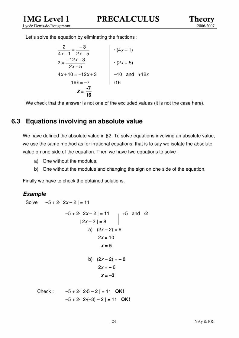
Let’s solve the equation by eliminating the fractions :
52
3
14
2
+
−=
− xx · (4x – 1)
52
3122
+
+−=
x
x · (2x + 5)
312104 +−=+ xx –10 and +12x
16x = –7 /16
x = -7
16
We check that the answer is not one of the excluded values (it is not the case here).
6.3 Equations involving an absolute value
We have defined the absolute value in §2. To solve equations involving an absolute value,
we use the same method as for irrational equations, that is to say we isolate the absolute
value on one side of the equation. Then we have two equations to solve :
a) One without the modulus.
b) One without the modulus and changing the sign on one side of the equation.
Finally we have to check the obtained solutions.
Example
Solve –5 + 2·| 2x – 2 | = 11
–5 + 2·| 2x – 2 | = 11 +5 and /2
| 2x – 2 | = 8
a) (2x – 2) = 8
2x = 10
x = 5
b) (2x – 2) = – 8
2x = – 6
x = –3
Check : –5 + 2·| 2·5 – 2 | = 11 OK!
–5 + 2·| 2·(–3) – 2 | = 11 OK!

1MG Level 1 PRECALCULUS Theory Lycée Denis-de-Rougemont 2006-2007
- 25 - YAy & PRi
6.4 Inequalities
An inequality is an equation where the « = » sign has been replaced by one of the
following signs : « ≤ , ≥ , <, > ». The solution is not a number any more but an interval.
Each time you divide or multiply the equation by a negative number you have to
change the direction of the inequality. The symbols « ≤ » and « ≥ » are called weak
inequalities and the symbols « < » and « > » are called strict inequalities.
Examples
a) Linear inequalities : Solve 4 7 13x− + < −
4 7 13 7
4 20 ( 4)
5
x
x
x
− + < − −
− < − ÷ −
>>>>
Division by a negative number
Finally the answer is : ] [5;x ∈ ∞
b) Quadratic inequalities : Solve 2 3 7 5x x− + ≥
The first step is to write all the x and all the numbers on the same side :
2
2
3 7 5 5
3 2 0
x x
x x
− + ≥ −
− + ≥
As a parabola changes its sign only when it intersects the x-axis we have to find
two solutions of the equation 2 3 2 0x x− + = . For that we use the quadratic
formula :
1
1,2
2
13 9 4 2
22
x
x
x
=± − ⋅
= =
=
↗
↘
Thanks to the two roots we can find the solution by making the sign table for 2 3 2 0x x− + = or sketching its graph. We want the x such that 2 3 2 0x x− + ≥ . It
is the grey cells :
x 1 2 2 3 2y x x= − + + 0 – 0 +
Finally the answer is : ] ] [ [;1 2;x ∈ − ∞ ∪ ∞
x
1 2

1MG Level 1 PRECALCULUS Theory Lycée Denis-de-Rougemont 2006-2007
- 26 - YAy & PRi
6.5 System of inequalities
A system of inequalities is a group of many inequalities that have to be satisfied at the
same time. We solve such a system by using a graphic method. We start by drawing the
lines that form the system. Then we hatch the area that contains the points (x ; y) that
satisfy the system.
Example
Solve the system
2 32 3
12 4 2
2
y xy x
y x y x
≤ −≤ −
⇔ + > > − +
We draw the two lines of the system
2 3
12
2
y x
y x
= −
= − +
.
Now we hatch the the points (x ; y) that satisfie both inequalities. The couples (x ; y) which
satisfy 2 3y x≤ − are under and on the line ( ≤ ). The couples (x ; y) that satisfy
12
2y x> + are over the line (>). Finally, we obtain the grey area and the line in bold type.
12
2y x= − +
-4 -2 2 4 6 8 10
-10
-5
5
10
15
2 3y x= −

1MG Level 1 PRECALCULUS Theory Lycée Denis-de-Rougemont 2006-2007
- 27 - YAy & PRi
§7 Applications and functions
7.0 Applications
Definition Application
An application is a relation that associates to each element of a first set A (preimages)
one and only one element of a second set B (images).
We can illustrate this notion with a concrete example. We consider :
a relation : the flights of Swiss airline,
a set A : Madrid, Paris, London and Bern
a set B : The United States.
This relation is an application, if and only if, for each cities of A there is one and only one
flight to a state of The United States.
Examples
a)
Not an application
It is an application
Not an application
X
X
X
X
X
X
X
A B b)
X
X
X
X
X
X
X
A B c)
X
X
X
X
X
X
X
A B
A B

1MG Level 1 PRECALCULUS Theory Lycée Denis-de-Rougemont 2006-2007
- 28 - YAy & PRi
d) A = { The students of the group 111 }, B = � and R (relation) = “To be born in …”
Yes it is an application because every student has a unique birth date.
e) A = { The students of the group 111 }, B = A and R = “To be taller than …”
No it is not an application because Léon is taller than Roxane and Caroline.
7.1 Functions
Definition Function
A function f is an application where A and B are sets of numbers.
Notation A → B
x � y = f(x)
Examples
a) A = B = �
f : x � y = x + 2 It is a function
f : x � y = x – 1 It is not a function : 0 – 1 = –1∉� so 0 doesn’t have
any image.
b) A = B = �
f : x � y = x – 2 It is a function
f : x � y = 2
2−x It is not a function :
5 2 3
2 2
−= ∉� so 5 doesn’t have
any image.
c) A = B = �
f : x � y = x – 3
2 It is a function
f : x � y = x
1 It is not a function, 0 doesn’t have any image
(division by zero).
d) A = B = �
f : x � y = x It is not a function, negative numbers don’t have any
image.
e) A = B = +�
f : x � y = x It is a function
f

1MG Level 1 PRECALCULUS Theory Lycée Denis-de-Rougemont 2006-2007
- 29 - YAy & PRi
Definition Domain
The domain D of a function f is the set of x (often x ∈ � ) for which the function f(x)
exists.
Examples
a) f(x) = 2
2−x Df = �
b) f(x) = 4
32 −x
Df = { }\ 2±�
c) f(x) = x−1 Df = ] ] ] ]\ 1 ; ; 1∞ = − ∞�
Definition Range
The range of a function f is the set of all values produced by the function f. Sometimes
we call it the image.
Definition Graph
The graph of a function f : A → B
x � y = f(x)
is the collection of all pairs (x, f(x)) = (x ; y) of the function, where x belongs to A and y
belongs to B. In particular, graph means the graphical representation of this collection, in
the form of a curve, together with axes.
Definition Injective function or injection
An injective function or injection is a function which maps distinct input values to
distinct output values. More formally, a function f : A → B is injective if, for every y in B
there is at most one x in A with f(x) = y.
Examples
Not an injection It is an injection
a)
X
X
X
X
X
X X
A B b)
X
X
X
X
X
X
X
A B

1MG Level 1 PRECALCULUS Theory Lycée Denis-de-Rougemont 2006-2007
- 30 - YAy & PRi
Definition Surjective function or surjection
A surjective function or surjection is a function with the property that all possible
output values of the function are generated when the input ranges over all the values in
the domain. More formally, a function f : A → B is surjective if, for every y in B, there is at
least one x in A with f(x) = y.
Examples
It is a surjection Not a surjection
Definition Bijective function or bijection
A function f : A → B is a bijection or one-one if it is both injective and surjective. This
means that for each number y in B there is only one number x in A with y = f(x).
Examples
Not a bijection It is a bijection Not a bijection
d) f : →� �
x � y = 0,5x – 2
It is a bijection
e) f : →� �
x � y = x2
Not a bijection, because it is not an injection nor a surjection, but if is
defined like that : f : + +
→� � it is a bijection.
X
X
X
X
X
X X
a) A B
b) X
X
X
X
X
X
X
A B
a)
X
X
X
X
X
X X
B A b)
X
X
X
X
X
X
B A c) X
X
X
X
X
X
X
B A

1MG Level 1 PRECALCULUS Theory Lycée Denis-de-Rougemont 2006-2007
- 31 - YAy & PRi
7.2 Inverse function
If a function is a bijection, then an inverse function (fonction réciproque) exists and we
note it if. It is defined from B to A. It allows us to “come back” :
f : A → B if : B → A
x � y = f(x) y � x = if(y)
Remark
We know that an inverse function exists only if the function is a bijection. Thus we should
check, before any calculations, that the function is a bijection. However it is not always an
easy exercise. So we are going to simplify this problem by supposing that the functions
we inverse are bijections. If it is not the case we calculate the inverse function and after
that we choose the domain and the range to make a bijection.
Examples
a) For easy bijections from →� � such as 3 2, 5 7, ...y x y x= − = − + it is easy to
find an inverse function. For that, we break up the function. Let’s consider, for
example, the function ( ) 4 6f x x= − . It is built like that :
4 64 4 6x x y x⋅ −→ → = −
To find the inverse function, we have to make the inverse operations of « 4⋅ »
and « – 6 » that are « 4÷ » and « + 6 ». We still have to determine in which
order we have to implement them. To answer this question compare this situation
with the fact of getting dressed. Firstly we put our socks ( 4⋅ ) and then our shoes
(– 6). When we get undressed, we take off our shoes (+ 6) and then our socks
( 4÷ ). It is now possible to find the inverse function of ( ) 4 6f x x= − :
6 4 64 6 6 4
4
yy x y x x+ ÷ +
= − → + = → =
We rename this function to obtain : 6
( )4
i xf x y
+= =
f if
x y
A B f
if

1MG Level 1 PRECALCULUS Theory Lycée Denis-de-Rougemont 2006-2007
- 32 - YAy & PRi
As the lines are bijections from →� � , we don’t have to find the domain and the
range.
b) For rational functions, the method is always the same, we have to express x in
terms of y. Let’s consider an example : 2
2
xy
x
−=
+.
2( 2)
2
( 2) 2 distributivity
2 2 and 2
2 2 factorize
( 1) 2 2 ( 1)
2 2
1
xy x
x
y x x
yx y x x y
yx x y
x y y y
yx
y
+= ⋅ −
−
− = +
− = + − +
− = +
− = + ÷ −
+=
−
We rename it to obtain : 2 2
( )1
i xf x y
x
+= =
−
The domain of ( )i f x is : { }\ 1i fD = �
Finally :
{ } { }: \ 2 \ 1
2
2
f
xx y
x
→
+=
−
� �
� is a bijection.
Its inverse function is :
{ } { }: \ 1 \ 2
2 2
1
i f
xx y
x
→
+=
−
� �
�
c) We proceed exactly as above for irrational functions. Let’s consider an
example : 2 4 1y x= − + .
2
2
2
2
2 4 1 1
1 2 4 ( )
( 1) 2 4 4
( 1) 4 2 2
( 1) 4
2
y x
y x
y x
y x
yx
= − + −
− = −
− = − +
− + = ÷
− +=
We rename it and we obtain : 2( 1) 4
( )2
i xf x y
− += =

1MG Level 1 PRECALCULUS Theory Lycée Denis-de-Rougemont 2006-2007
- 33 - YAy & PRi
d) The last kind of functions that we are going to consider in order to find their
inverse function is the quadratic functions. We have to start by writing the
quadratic in completed square form. As in the other examples, let’s work with an
example: 2 2y x x= − . The completed square form is 2( 1) 1y x= − − . It is now
possible to find its inverse function :
2
2
( 1) 1 1
1 ( 1)
1 1 1
1 1
y x
y x
y x
x y
= − − +
+ = −
+ = − +
= + +
The function :
[ [ [ [
2
: 1; 1;
2
f
x y x x
∞ → − ∞
= −� is a bijection.
Its inverse function is :
[ [ [ [: 1; 1;
1 1
i f
x y x
− ∞ → ∞
= + +�
Remark
If f is a one–one function or bijection, then the graphs of y = f(x) and y = if(x) are
reflections of each other in the line y = x.
7.3 Composite function
Since secondary school, we know how to compose symmetries, rotations, translations, etc
together. Now we are going to learn how to compose functions. Given two functions f and
g. We define the composite function (fonction composée) of f and g, in this order, like
that :
( )( ) ( ( ))g f x g f x∗ =
Example
Given the functions ( ) 2 4f x x= − and 2( ) 3g x x= . Calculate andg f f g∗ ∗ .
2 2 2( )( ) ( ( )) (2 4) 3(2 4) 3(4 16 16) 12 54 54g f x g f x g x x x x x x∗ = = − = − = − + = − +
2 2 2( )( ) ( ( )) (3 ) 2 3 4 6 4f g x f g x f x x x∗ = = = ⋅ − = −
1MG Level 1 PRECALCULUS Theory Lycée Denis-de-Rougemont 2006-2007
- 34 - YAy & PRi
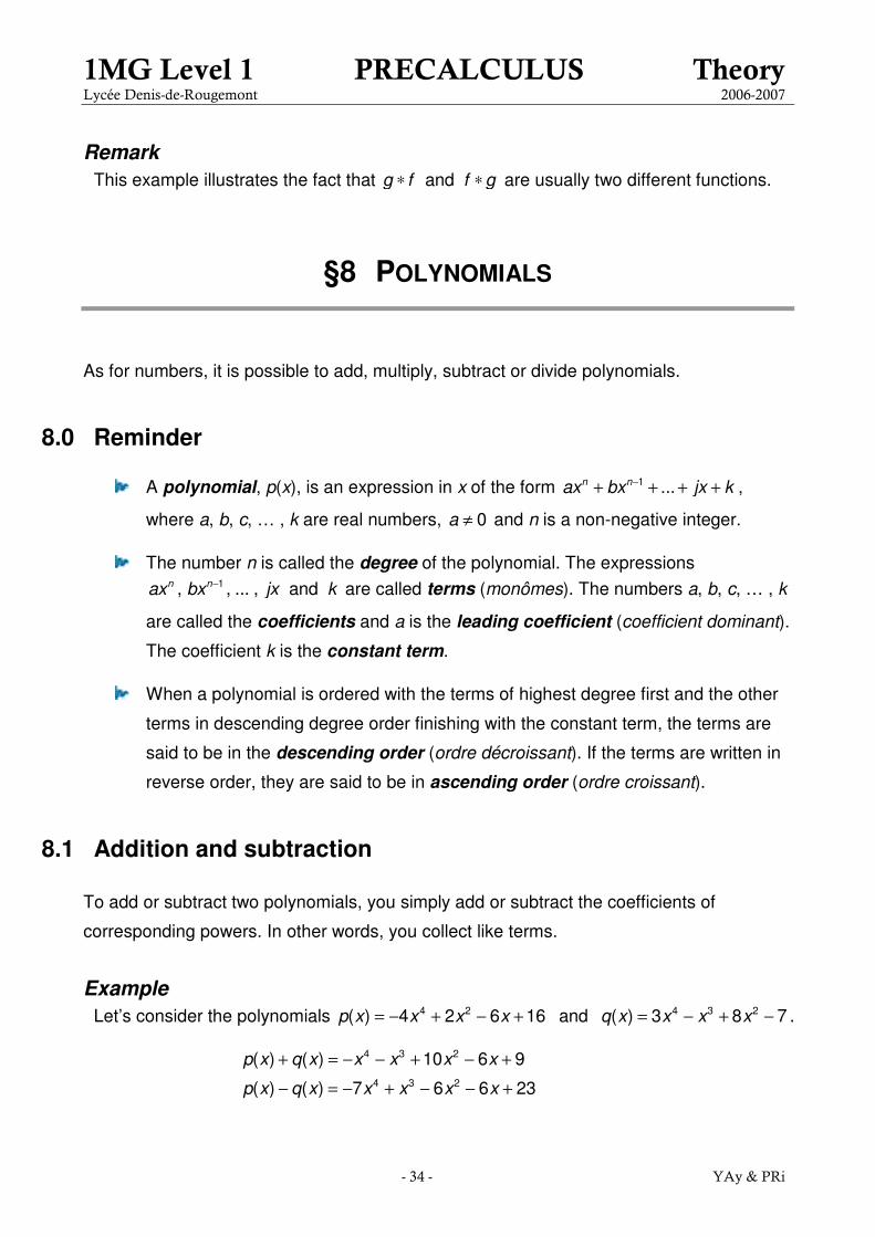
Remark
This example illustrates the fact that andg f f g∗ ∗ are usually two different functions.
§8 POLYNOMIALS
As for numbers, it is possible to add, multiply, subtract or divide polynomials.
8.0 Reminder
A polynomial, p(x), is an expression in x of the form 1 ...n nax bx jx k−+ + + + ,
where a, b, c, … , k are real numbers, 0a ≠ and n is a non-negative integer.
The number n is called the degree of the polynomial. The expressions 1, , ... , andn nax bx jx k− are called terms (monômes). The numbers a, b, c, … , k
are called the coefficients and a is the leading coefficient (coefficient dominant).
The coefficient k is the constant term.
When a polynomial is ordered with the terms of highest degree first and the other
terms in descending degree order finishing with the constant term, the terms are
said to be in the descending order (ordre décroissant). If the terms are written in
reverse order, they are said to be in ascending order (ordre croissant).
8.1 Addition and subtraction
To add or subtract two polynomials, you simply add or subtract the coefficients of
corresponding powers. In other words, you collect like terms.
Example
Let’s consider the polynomials 4 2 4 3 2( ) 4 2 6 16 and ( ) 3 8 7p x x x x q x x x x= − + − + = − + − .
4 3 2( ) ( ) 10 6 9p x q x x x x x+ = − − + − +
4 3 2( ) ( ) 7 6 6 23p x q x x x x x− = − + − − +

1MG Level 1 PRECALCULUS Theory Lycée Denis-de-Rougemont 2006-2007
- 35 - YAy & PRi
8.2 Multiplication
When we multiply polynomials it is fundamental to bear in mind that the multiplication is
distributive over the addition, this means that all the terms of the right parenthesis are
multiplied by all the terms of the left parenthesis. We multiply the coefficients between
them and the rules of indices tell us that we have to add the degrees. Finally we add the
terms in x that have the same degree.
Example
Given two polynomials 4 2 2( ) 4 2 16 and ( ) 2 1p x x x q x x= − + + = − , then
2 4 2 6 4 2 4 2
6 4 2
( ) ( ) (2 1)( 4 2 16) 8 4 32 4 2 16
8 8 30 16
p x q x x x x x x x x x
x x x
⋅ = − − + + = − + + + − − =
= − + + −
8.3 Long Division
The problem we have to solve is to divide 4 3 22 3 5 7x x x x− + + − by 2x + . For that, we
are going to copy the division of two numbers. Let’s divide 67 by 5 :
67 5
(65) 13
2
quotient
remainder
− =
=
We can write : 67 5 13 2= ⋅ +
If we apply this method to polynomials we obtain the following process :
1st step We consider only the terms of highest degree 42x :
42 :x x the result is 32x
So we write :
4 3 22 3 5 7x x x x− + + − 2x +
32x
2nd step We multiply 2+x by 32x the result is 4 32 4x x+
Then we write :
4 3 22 3 5 7x x x x− + + − 2x +
4 32 4x x+ 32x

1MG Level 1 PRECALCULUS Theory Lycée Denis-de-Rougemont 2006-2007
- 36 - YAy & PRi
3rd step SUBTRACT 4 32 4x x+ from 4 3 22 3 5 7x x x x− + + −
We obtain :
4 3 22 3 5 7x x x x− + + − 2x +
4 3(2 4 )x x+−−−− 32x
3 27 5 7x x x− + + −
Next step Repeat those three steps with the new term of highest degree 37x− :
( )3 27 : 7x x x− = − and ( )2 3 27 ( 2) 7 14x x x x− ⋅ + = − −
Thus :
4 3 22 3 5 7x x x x− + + − 2x +
4 3(2 4 )x x+−−−− 3 22 7x x−
3 27 5 7x x x− + + −
3 27 14x x− −
SUBTRACTION : ( ) ( )3 2 3 2 27 5 7 7 14 19 7x x x x x x x− + + − − − − = + −
4 3 22 3 5 7x x x x− + + − 2x +
4 3(2 4 )x x+−−−− 3 22 7x x−
3 27 5 7x x x− + + −
3 2( 7 14 )x x− −−−−−
219 7x x+ −
Repeat these three steps with the new term of highest degree 219x :
( )219 : 19x x x= and 219 ( 2) 19 38x x x x⋅ + = +
We have :
4 3 22 3 5 7x x x x− + + − 2x +
4 3(2 4 )x x+−−−− 3 22 7 19x x x− +
3 27 5 7x x x− + + −
3 2( 7 14 )x x− −−−−−
219 7x x+ −
2(19 38 )x x+−−−−
37 7x− −
NEW
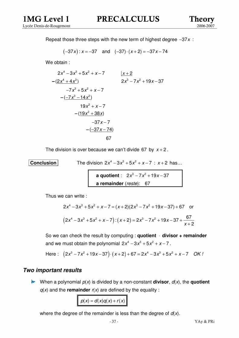
1MG Level 1 PRECALCULUS Theory Lycée Denis-de-Rougemont 2006-2007
- 37 - YAy & PRi
Repeat those three steps with the new term of highest degree 37x− :
( )37 : 37x x− = − and ( 37) ( 2) 37 74x x− ⋅ + = − −
We obtain :
4 3 22 3 5 7x x x x− + + − 2x +
4 3(2 4 )x x+−−−− 3 22 7 19 37x x x− + −
3 27 5 7x x x− + + −
3 2( 7 14 )x x− −−−−−
219 7x x+ −
2(19 38 )x x+−−−−
37 7x− −
( 37 74)x− −−−−−
67 The division is over because we can’t divide 67 by 2x + .
Conclusion The division 4 3 22 3 5 7x x x x− + + − : 2x + has…
a quotient : 3 22 7 19 37x x x− + −
a remainder (reste): 67
Thus we can write :
4 3 2 3 22 3 5 7 ( 2)(2 7 19 37) 67x x x x x x x x− + + − = + − + − + or
( ) ( )4 3 2 3 2 672 3 5 7 : 2 2 7 19 37
2x x x x x x x x
x− + + − + = − + − +
+
So we can check the result by computing : quotient ⋅ divisor + remainder
and we must obtain the polynomial 4 3 22 3 5 7x x x x− + + − .
Here : ( ) ( )3 2 4 3 22 7 19 37 2 67 2 3 5 7x x x x x x x x− + − ⋅ + + = − + + − OK !
Two important results
When a polynomial p(x) is divided by a non-constant divisor, d(x), the quotient
q(x) and the remainder r(x) are defined by the equality :
( ) ( ) ( ) ( )p x d x q x r x= +
where the degree of the remainder is less than the degree of d(x).

1MG Level 1 PRECALCULUS Theory Lycée Denis-de-Rougemont 2006-2007
- 38 - YAy & PRi
Let p(x) be a polynomial. Then
If x t− is a factor of p(x), i.e. ( ) ( ) ( )p x x t a x= − ⋅ then p(t) = 0 (t is a zero or
solution of p(x)).
If p(t) = 0, i.e. t is a solution or zero of p(x), then x t− is a factor of p(x) so we
can write : ( ) ( ) ( )p x x t a x= − ⋅ where a(x) is the quotient of the division of p(x)
by x t− . This is the factor theorem.
In other words, if t is a zero or solution of p(x), then p(x) is divisible by x t− .
If p(x) is divisible by x t− then t is a zero or solution of p(x).
§9 EXPONENTIAL AND LOGARITHMIC FUNCTIONS
9.0 Definition and properties
Here are the graphs of 10 , Log( ) andxy y x y x= = =
As these graphs are symmetrical about the line
xy = , we deduce that (cf. 7.2) :
Log( ) and 10xx are inverse functions.
This means : ( )x Log( )Log 10 and 10 xx x= =
A function of the form ( ) where , 0xf x b x b= ∈ >� is called an exponential function.
We call Log logarithm to base 10 (logarithme de base 10). Calculating Log(b) means looking for
the power to which we have to rise 10 to find b. Actually :
3Log(0,001) 3 10 0,001 −= − ⇔ =
It is possible to calculate logarithm to any base, but here we are going to consider only the
base 10. Using Log, it is now possible to solve new equations. For that we use a property
of logarithm :
Log( ) Log( )ba b a= ⋅
-2 2 4
-3
-2
-1
1
2
3
4
5
10xy=
Log( )y x=
y x=

1MG Level 1 PRECALCULUS Theory Lycée Denis-de-Rougemont 2006-2007
- 39 - YAy & PRi
Let’s check this with 3 and 5a b= = : 5Log(3 ) Log(243) 2,38= ≅ and 5 Log(3) 2,38⋅ ≅
Thanks to the multiplication rule, it is now possible to solve equations like : 114 =x
4 11 Log
Log(4 ) Log(11) rule
Log(4) Log(11) Log(4)
Log(11)1,73
Log(4)
x
x
x
x
=
=
⋅ = ÷
= ≅
Verification : 1,73...4 11 !OK=
As exponential and logarithmic functions are inverse function, it is also possible to solve
for instance Log( ) 2x = :
Log( ) 2
Log( ) 2 10
10 10
100
x
x
x
inverse functions
x
=
=
=
Verification : Log(100) 2 !OK=
Remark
These two new functions are used in domains as chemistry, biology or economy as well.
Actually, the growth of a bacteria population, the decomposition of a radioactive element
or the banking interests can be described by exponential functions.
Another concrete example is the Richter scale which measures the power of an earthquake. It is
a logarithmic scale : the magnitude of Richter corresponds to the logarithm of the amplitude of
the vibrations recorded by a seismograph calibrated according to the distance from the
epicentre. Thus, for example, this means that an earthquake of magnitude 6 is 10 times more
powerful than a seism of magnitude 5.
Recommended